


The paper applies the concept of identity to investigate whether consumer behavior matters for a household's financial security. It is assumed that considerable part of households may express their identity through status-oriented consumption. The research is carried out in two steps. First, the index of financial security is built and used to determine the level of financial security experienced by working-age families in Poland. Second, the simulation results based on an econometric model are employed to find the answer to the question: Does financial insecurity result more from the need to manifest consumption at the higher level than average in an income-group of which people are members, or people want to be distinguishable inside their own income-group but they do not identify with a group having consumption at visibly higher level, or from the need to improve self-image by bringing own consumption closer to the pattern of a group with higher wealth status of which they are not members? The source of data is the 2005-2009 Households Budget Surveys in Poland. The findings offer empirical evidence for the relevance of consumer behavior for financial security of households in Poland. Considerable part of households expresses identity through conspicuous consumption. Both groups of households, the insecurity rich and the insecurity poor, accept the same ranking of status goods: a car on the first position, next homes (housing and equipment) and clothes on the third place. Status-oriented consumption creates life beyond means and pushes even relatively rich households towards financial insecurity.
El trabajo aplica el concepto de identidad a investigar si el comportamiento del consumidor es importante para la seguridad financiera de un hogar. Se asume que parte considerable de los hogares pueden expresar su identidad por medio de un consumo orientado al estatus. La investigación se realiza en dos pasos. Primero, se construye y se usa el índice financiero para determinar el nivel de seguridad financiera que gozan las familias en edad laboral en Polonia. Segundo, se emplean los resultados de la simulación, basados en un modelo econométrico, para encontrar la respuesta a la cuestión: ¿Es la inseguridad financiera un resultado más de la necesidad de manifestar el consumo al nivel más alto que el promedio en un grupo de ingresos del que son miembros las personas, o quieren las personas distinguirse dentro de su propio grupo de ingreso pero no se identifican con un grupo con un consumo a un nivel visiblemente más alto, o es resultado de la necesidad de mejorar la autoimagen acercando más el propio consumo al patrón de un grupo con un estatus de riqueza más alto del que ellos no son miembros? La fuente de los datos es la Encuesta 2005-2009 de Presupuestos del Hogar en Polonia. Los resultados ofrecen evidencia empírica para la relevancia del comportamiento del consumidor para la seguridad financiera de los hogares en Polonia. Una parte considerable de los hogares expresa su identidad mediante un consumo notorio. Ambos grupos de hogares, los inseguros ricos y los inseguros pobres, aceptan la misma clasificación de bienes del estatus: un carro en primer lugar, en seguida, una casa (habitación y equipamiento) y ropa, en tercer lugar. El consumo con orientación al estatus crea una vida más allá de los medios y arrastra incluso a los hogares relativamente ricos hacia la inseguridad financiera.
The household's identity (a household is treated as the whole) shapes consumer behavior and affects the household's choice of a consumption pattern. The concept of identity has been introduced into economics by Akerlof and Kranton (2000, 2005) and by Davis (2003, 2007). Akerlof and Kranton have focused on the social identity drawn directly from social psychology and self-categorisation theory. They have incorporated the social identity as an argument in the utility function. Davis has employed the sociological approach to identity and suggested to treat the individual as being active in creating a personal identity. The purpose of the paper is to apply the concept of identity (mainly social identity) to investigate the importance of consumer behavior for financial security of households in Poland.
The structure of the paper is as follows: the research concept is presented in the first section; the methodology in the second; findings in the third and finally the conclusions.
Research conceptAkerlof and Kranton, in their book “Identity economics”, have given the following definition of the term “identity” and its relations to social categories and norms: “People's identity defines who they are-their social category. Their identities will influence their decisions, because different norms for behavior are associated with different social categories. First, there are social categories (…). Second, there are norms for how someone in those social categories should or should not behave. Third, norms affect behavior” (Akerlof & Kranton, 2010, p. 13). Social categories are broad social science classifications used to describe widely recognized social aggregates (Davis, 2007, p. 350). In the Akerlof-Kranton framework the social identity means that individuals identify with people in same categories and differentiate themselves from those in others (Akerlof & Kranton, 2000, p. 720).
The social identity is based on the idea of “identifying with” others, while the personal identity on the idea of “identity apart from” others. Individuals have personal identities as well as social identities, and these two concepts are related as Davis has emphasized (Davis, 2007, p. 355). He has suggested to see personal identity as being fundamental in the sense that individual creates his/her identity, considering the utilities drawn from multiple social identities. The Davis extension of the Akerlof and Kranton utility function by incorporating, additionally, personal identity, makes identity reflective in the sense that the individual evaluates the utility created by social identity, taking into account how this utility contributes to their personal identity.
Consumption is related to the process of identity formation by signaling status. First, consumption points at the reference groups with which people want to identify. Second, relative status determines patterns of behavior (such as for example white or blue collar habits) (Herrmann-Pillath, 2008).
A reference group is a group of people (or even a person) that significantly influences an individual's behavior. Such an influence can appear when people orient themselves to other than membership groups in shaping their behavior and evaluations (Merton & Rossi, 1949). Reference groups unmask people's preferences on behavior and lifestyles, influence self-concept development, contribute to the formation of values and attitudes, and generate pressure for conformity to group norms (Bearden & Etzel, 1982). Kelley (1947) distinguished between reference groups used as standards of comparison for self-appraisal (comparative) and those used as a source of personal norms, attitudes and values (normative).
Based on the work of Deutsch and Gerard (1955) and Kelman (1961), information, utilitarian and value-expressive influences can be identified. Informational influence can flow from a need to be a properly informed. Those who offer information influence others. Utilitarian reference group influence appears if an individual feels that it will be useful to meet the expectations of people significant for him or her. Value-expressive influence is characterized by the need for psychological association with a person or group and is reflected in acceptance of positions expressed by others. This association can take two forms: being like the reference group or liking for the reference group.
The reference group construct is important in at least some types of consumer decision making. Many individuals can manifest their identity thorough consumption. They may derive utility from the consumption of commodities. Consumption can be seen through status goods that are defined according to their meanings, not to their functions. Their utility depends on the interactions in social networks which manifest status orders. As Herrmann-Pillath (2008) emphasizes status goods entirely depend on the cultural frame in the sense that everything can be a status good. Even consumption of foodstuffs influences the process of identity formation.
Akerlof and Kranton argue that individual utility is partly determined by the extent to which one perceives to conform with certain social types to which one strives to belong. In the same sense Potts, Cunningham, Hartley, and Ormerod (2008) define social network goods as goods in which individual utility is partly determined by the extent to which others also consume the same good. Consumption of such social network goods leads toward collective patterns of consumption.
Osberg (1998) points that that the maintenance of social identity depends partially on whether or not individuals have the discretionary income to purchase goods and services perceived as appropriate to manifest their identity. Economic insecurity about outcomes can, therefore, be highly threatening to the individual's identity.
The paper addresses the inverse influence, it means, the influence of identity on a household's financial security.1 The household's identity (a household is treated as the whole) shapes consumer behavior and affects the household's choice of a consumption pattern.
The research is carried out under the assumptions that (1) households appreciate consumption and then a group characterized by high levels of consumption will have a higher status than a group characterized by low levels; (2) for some households consumption expenditure may be more important than income, as a criterion, when they compare themselves.
The purpose of the paper is to apply the concept of identity (mainly social identity) to investigate whether consumer behavior matters for financial security of households in Poland. People can be motivated to buy any good by a need to manifest consumption at the higher level than the average in an income-group of which people are members, or people want to be distinguishable inside of own income-group but they do not identify with members of own groups having the highest consumption expenditure. A need to improve his/her self-image by having consumption at the highest level in own-income group can drive consumer behavior of the other. Some people can feel very strongly a need to bring own consumption closer to the pattern of a group with higher wealth status of which they are not members. These people want to create the impression of attachment to the group with higher consumption rather than to be associated with this group. The research tries to reveal which of those needs is the most important to explain the differentiation in financial security across households in Poland. The findings should also reveal which goods are considered status goods by households in Poland.
MethodologyThe research is carried out in two steps. First, the index of financial security is built to determine the level of financial security experienced by working-age families in Poland. Second, the simple simulation based on the regression estimation is applied to find answers to the research questions (presented above) related to the influence of consumer behavior on financial insecurity.
The index of financial security of householdsIn the literature there are two concepts: economic security and economic insecurity. Scientists define economic insecurity concentrating on either existence of current losses (Hacker, 2007) or anxiety, fear connected with the possibility of occurrence of such losses in the near future (Anders & Gascon, 2007; Dominitz & Manski, 1997; Osberg, 1998). In contrary security is regarded as the fulfillment of certain conditions which guarantee the individual wealth (Beeferman, 2002; report By a Thread: The New Experience of America's Middle Class (2007) prepared together by Demos: A Network for Ideas & Action and The Institute on Assets and Social Policy at Brandeis University; ILO Socio-Economic Security Programme).
Financial security is defined very narrowly in the paper as the ability to achieve income necessary for covering household needs at its suitable level and to create financial reserves to be at disposal in case of unfavorable accidence (sickness, job loss, family breakdown).
Source of data: Household Budget Survey (HBS) conducted by the Polish Central Statistical Bureau for the panel of 2005–2006 and 2008–2009. Each household is included in the HBS over two years. The total number of households in the panel 2008–2009 is equal to 8034. The structure of the sample is as follows: 7049 households with income from hired work (3981 manual worker households and 3068 non-manual worker households), and 985 households with income from self-employment. The total number of households in the panel of 2005–2006 is equal to 7638.
Poland enjoyed very dynamic growth over the period of 2005–2008. The research period is chosen to investigate a change in consumer behavior that could matter for financial security between the beginning of economic prosperity (2005–2006) and the first wave of the financial crisis (2008–2009) three years later.
The methodology of the financial security index covers:
- •
defining a sample;
- •
identifying factors influencing financial security;
- •
setting weights for the factors in the index;
- •
setting for each area included in the index: (1) a threshold that would be optimal to support overall financial security, and (2) a threshold that would threaten it – finally, determining percentage of households that met these thresholds.
- •
defining criteria for considering the family: (1) secure, or (2) at high risk, or (3) in-between these two groups;
- •
calculating the index for each household.
The research is based on a sample covering households meeting two following criteria:
- •
main income source – households which main income source of maintenance is: income from hired work or income from self-employment (employees and owners of small and medium-sized firms, lawyers, artists, journalists; excluding farmers); all incomes are considered equivalent incomes; the modified OECD scale is used: 1 for the first adult person in household, 0.5 for each next member of household – 14 years and over, 0.3 – for every child under 14 years.
- •
age range – age of household head: 25–64 (working age for a man with the university's diploma)
The whole sample, based on these two criteria, is divided into sub-samples called “the rich” and “the poor”. The threshold for income is set as 150% of social minimum (adjusted to a household size using the OECD scale). Social minimum is not a poverty line. It constitutes income that allows to keep living standards at the minimum but fair level, including not only biological but also social needs. Social minimum is calculated by the Institute of Labour and Social Studies. For example, in 2009 the 150% of social minimum for a 4-person family was equal to 1844 PLN≈461 EUR (an equivalent income per person per month).
Identifying factors influencing financial security and setting the weights and thresholds for themThe index covers three factors: financial assets, housing and budget. All three factors are crucial for financial security defined narrowly in this paper. Each factor is included in the index with its weight that reflects its relevance for overall financial security. The weight depends on the percentage of households that meets the threshold of risk for financial security.
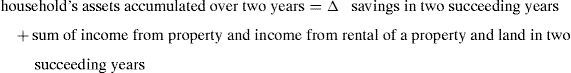
Assets are the key factor of financial security. The problem occurs how to estimate household's assets when data on savings, securities as well as on home equity are not available at a household's level. It seems to be acceptable to investigate whether a household has been able to generate savings over two succeeding years (a given household is included in the HBS only over two years). Basing on this proposal the 2-year sum of an increase in savings plus capital income has been applied as a proxy of assets accumulated over two years; in details:
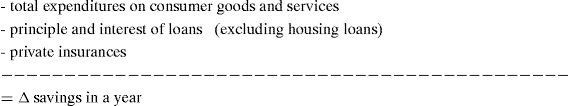
An increase in savings is calculated as a surplus of available income over total consumer expenditures and loan repayment and private insurances; in details:
income from hired work or income from self-employment
The asset factor is included in the index as the number of months when a family could meet 75% of its essential living expenses, using financial assets accumulated over two last years (the increase in assets calculated as above).
Essential living expenses are expenditures on food, housing (without spending on furniture and equipment), clothing, transport (without purchases of cars and motors, bicycles), health care, personal care, education, transport insurance, private health insurance.
Setting the thresholds is based on the average number of months without income from hired work or self-employment. This number of months depends on the situation in a labor market and it was equal to 10 months in 2009. Therefore:
- -
The optimal level for financial security – the level of assets accumulated over two last years that allows a family to cover 75% of its essential living expenses for at least 150% of average number of months without employment income or income from self-employment;
- -
Risk for financial security – the level of assets accumulated over two last years that allows to finance 75% of its essential expenses for less than 50% of average number of months without employment income or income from self-employment.
The housing factor means a percentage of after-tax income spent on housing.
Housing expenses: mortgage principle and interest for owned home/or vacation home, rent, insurance, maintenance, utilities, fuels and public services.
In absence of the Polish definition of housing affordability the thresholds are based on the definition used by the Department of Housing and Urban Development in USA. This definition can be also accepted in Polish conditions.
- -
The optimal level for financial security – less than 20% of after-tax income spent monthly on housing;
- -
Risk for financial security – more than 30% of after-tax income spent monthly on housing
The budget factor is included into the index as the ratio of the amount left at the end of the month after paying taxes and covering living expenses to the amount that allows to make ends meet. This amount should afford a family to cover the costs of expensive medicines, to improve housing, or in general, to improve the quality of life or saving and investing.
In details:

- -
total consumer expenditures
- -
principle and interest of loans and house loans
- -
house, life, health and other private insurances
An amount that allows to make ends meet is a base for the thresholds. In 2009 this amount was equal to 806 PLN per month/per equivalent person (≈202 EUR).
- -
The optimal level for financial security – Amount left at the end of the month after paying taxes and covering living costs is more than 150% of the amount that allows to make ends meet (the amount adjusted to a family size);
- -
Risk for financial security – Amount left at the end of the month after paying taxes and covering living costs is less than 50% of the amount that allows to make ends meet (the amount adjusted to a family size).
A family can enjoy financial security, if at least two factors for this family meet the optimal threshold for financial security. A family is exposed to financial insecurity, if at least two factors for this family meet the threshold defined as risk for financial security. If a family falls between these two groups it means that the family is not at high risk but its financial security is fragile.
Calculating the financial security indexThe financial security index for each household is calculated as follows:
where:
FSi – financial security index for i household; i=1…N; N=8034
Ai – asset factor as the number of months when a family could meet 75% of its essential living expenses, using financial assets accumulated over two last years
Hi – housing factor means the percentage of after-tax income spent on housing
Bi – budget factor as the ratio of the amount left at the end of the month after paying taxes and covering living expenses to the amount that allows to make ends meet.
wij – weight for j factor and i household: j=asset, housing, budget
The values of each factor are normalized relative to its average. The weights are based on the percentage of households that met the threshold of risk to financial security. The weights are normalized relative to their sum. The higher value of the index means the higher level of financial security.
The econometric modelCharacteristics of the insecure poor and insecure richIn the second step of the research – for each panel data, 2005–2006 and 2008–2009 – the sample of insecure households (determined in the first step) in each panel is divided into groups:
- -
the insecure rich – households with an equivalent income above 150% of social equivalent minimum in a given year (N=1085 for 2005–2006 and N=1442 for 2008–2009)
- -
the insecure poor–households with an equivalent income below 150% of social equivalent minimum (N=4374 for 2005–2006 and N=3092 for 2008–2009)
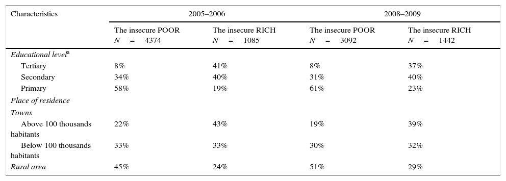
The group of the insecure poor covers households with visibly lower level of education, living in villages and small towns (see Table 1), while a considerable part of the insecure rich has the university diplomas and lives in big and medium-size towns.
Insecure households by an educational level and a place of residence in the panels of: 2005–2006 and 2008–2009 (in %).
| Characteristics | 2005–2006 | 2008–2009 | ||
|---|---|---|---|---|
| The insecure POOR N=4374 | The insecure RICH N=1085 | The insecure POOR N=3092 | The insecure RICH N=1442 | |
| Educational levela | ||||
| Tertiary | 8% | 41% | 8% | 37% |
| Secondary | 34% | 40% | 31% | 40% |
| Primary | 58% | 19% | 61% | 23% |
| Place of residence | ||||
| Towns | ||||
| Above 100 thousands habitants | 22% | 43% | 19% | 39% |
| Below 100 thousands habitants | 33% | 33% | 30% | 32% |
| Rural area | 45% | 24% | 51% | 29% |
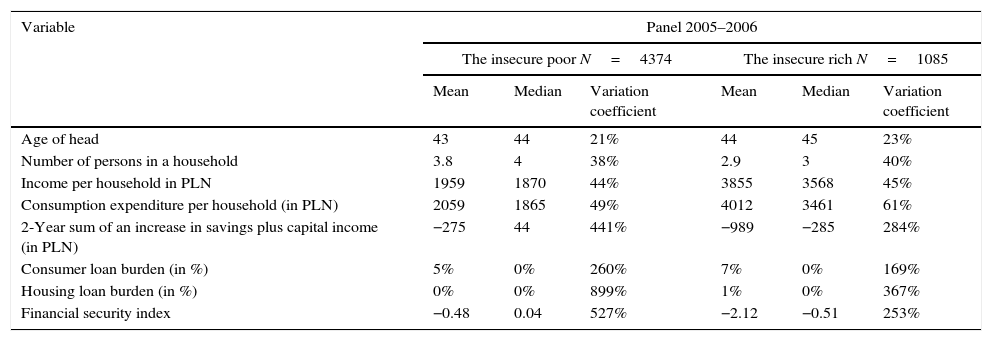
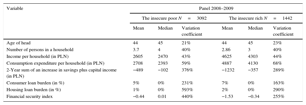
Descriptive statistics of main variables for the insecure poor and the insecure rich in the panels of 2005–2006 and 2008–2009 are presented in Tables 2 and 3, respectively. Age of a head in both groups of households and in both data panels is similar, more or less 44 years. A size of a household is a little bit smaller for the insecure rich (3 persons in average) than for the insecure poor (4 persons). Income per household is, of course, higher for the insecure rich but it is worth to mention that a difference between mean income and median income in both groups in both periods is rather small suggesting there is no significant income inequality among each group. A little bit bigger difference can be found in consumption expenditure, more visible for the insecure rich (a ratio of mean expenditure to median expenditure equals 1.16 in 2005–2006 and 1.18 in 2008–2009 while a ratio of mean income to median income is equal to 1.08 and 1.07, respectively).
Descriptive statistics of main variables for the insecure poor and the insecure rich in the panel of 2005–2006.
| Variable | Panel 2005–2006 | |||||
|---|---|---|---|---|---|---|
| The insecure poor N=4374 | The insecure rich N=1085 | |||||
| Mean | Median | Variation coefficient | Mean | Median | Variation coefficient | |
| Age of head | 43 | 44 | 21% | 44 | 45 | 23% |
| Number of persons in a household | 3.8 | 4 | 38% | 2.9 | 3 | 40% |
| Income per household in PLN | 1959 | 1870 | 44% | 3855 | 3568 | 45% |
| Consumption expenditure per household (in PLN) | 2059 | 1865 | 49% | 4012 | 3461 | 61% |
| 2-Year sum of an increase in savings plus capital income (in PLN) | −275 | 44 | 441% | −989 | −285 | 284% |
| Consumer loan burden (in %) | 5% | 0% | 260% | 7% | 0% | 169% |
| Housing loan burden (in %) | 0% | 0% | 899% | 1% | 0% | 367% |
| Financial security index | −0.48 | 0.04 | 527% | −2.12 | −0.51 | 253% |
Descriptive statistics of main variables for the insecure poor and the insecure rich in the panel of 2008–2009.
| Variable | Panel 2008–2009 | |||||
|---|---|---|---|---|---|---|
| The insecure poor N=3092 | The insecure rich N=1442 | |||||
| Mean | Median | Variation coefficient | Mean | Median | Variation coefficient | |
| Age of head | 44 | 45 | 21% | 44 | 45 | 23% |
| Number of persons in a household | 3.7 | 4 | 40% | 2.86 | 3 | 40% |
| Income per household (in PLN) | 2605 | 2470 | 43% | 4625 | 4303 | 44% |
| Consumption expenditure per household (in PLN) | 2708 | 2393 | 59% | 4887 | 4130 | 68% |
| 2-Year sum of an increase in savings plus capital income (in PLN) | −489 | −102 | 376% | −1232 | −357 | 289% |
| Consumer loan burden (in %) | 5% | 0% | 231% | 7% | 0% | 163% |
| Housing loan burden (in %) | 1% | 0% | 593% | 2% | 0% | 290% |
| Financial security index | −0.44 | 0.01 | 440% | −1.53 | −0.34 | 255% |
Visible differentiation among each group and between two groups in both panels can be observed for a sum of increases in savings as well as for loan burden and finally for financial security index.
The two-year sum of increases in savings plus capital income is used to measure an ability of a household to increase its assets. If a household is not able to generate any surplus of income over its expenditure over two years, its financial security can be fragile. In both periods the insecure rich experienced dissavings (a decline in savings) to larger extend than the insecure poor. The statistics show, however, the visible increase in dissavings among the insecure poor in the period of 2008–2009. The high mean/median ratios as well as the high values of variation coefficients point at considerable concentration of dissavings in both groups of households. It means there are households extremely insecure due to this reason.
Loan burden can be a cause of financial insecurity only for a small number of households. Majority of insecure households do not have any loans. However a small part of those who are in debts can feel insecure. Variation of loan burden, especially in reference to housing loans, is very high.
The statistics of financial security index (the higher values of mean and median, higher financial security of households) show that a mean (and median) level of financial security is much lower for the insecure rich than insecure poor, while variation is stronger among the insecure poor.
VariablesFor each of these two groups of households in each panel the econometric model is estimated with the financial security index as the dependent variable. The reason to estimate the model for each panel is that a given household is included in the HBS only over two years.
A household is an observation unit, it means that identity of the household refers to the family's identity shaped by interactions between family members. An individual's decision about whether or not to buy a good may be influenced by the expectations of family members.
There are two groups of insecure households, the insecure rich and the insecure poor. Each insecure household is characterized by vector of expenses on consumer goods and services Gi=(Gi1…GiC)Gic, where i means an insecure household, i=1…N; and c means a category of consumer goods and services, c=1…C
A social group determined by the wealth status, (the rich or the poor) is characterized by two kinds of the prototype of consumption, Gjkc:
- 1)
Gjmc is equal to the mean expenses (m) on c category of goods and services across members of j group (the rich group or the poor group); or
- 2)
Gjhc is equal to the average of ten highest expenses (h) on c across members of j group
Gjkc, where j means a group (the rich=r, or the poor=p); k means a kind of the prototype for consumption of c category of goods and services; k can be, m, the mean expenses across members of the whole rich group, r, (or of the whole poor group, p) and h, the highest expenses (precisely, the average of ten highest expenses) across members of the whole rich group, r, (or of the whole poor group, p). The prototype of consumption is based on the consumption of the rich, as the whole and on the consumption of the poor, as the whole, not on the consumption of insecure households.
The research covers 12 categories of consumption expenditure:
- -
Food and non-alcoholic beverages
- -
Alcoholic beverages, tobacco
- -
Clothing and footwear
- -
Housing, water, electricity, gas and other fuels
- -
Furnishings, household equipment and routine maintenance of the house
- -
Health
- -
Transport
- -
Communication
- -
Recreation and culture
- -
Education
- -
Restaurants and hotels
- -
Hygiene
The main independent variables measure the 2-year sums of weighted distances between the insecure household's expenses on particular categories of consumer goods and services and the levels of expenses described as the prototypes of consumption.
First, the distance between the insecure household's expenses and the mean expenses in its income group (it means the rich or the poor). Such the distance is assumed to reflect the need to be distinguishable inside of own income-group by having consumption at higher level than the own-group average but without liking for expenditure at the top.

Second, the distance between the insecure household's expenses and the expenses made by the group with higher material status. This distance reflects the need to create the impression of attachment to the group with higher consumption rather than a desire to be associated with this group.
- -
for the insecure poor – the distance between the insecure household's expenses:
- -
the mean expenses of the rich
or
- -
the highest expenses of the rich
Third, the distance between the insecure household's expenses and the highest expenses in own group. This distance describes the need to improve household's self-image by having consumption at the highest level in own group;
- -
for the insecure rich – the distance between the household's expenses and the highest expenses across members of the rich:
- -
for the insecure poor – the distance between the household's expenses and the highest expenses across members of the poor:
Fourth, the distance between the insecure rich household's expenses and the highest expenses of the poor (the highest expenses across members of the poor are at visibly higher level than mean expenses for the rich, and of course, they are lower than the highest expenditure made by the rich). This distance is assumed to show that some households may evaluate that a group characterized by high levels of consumption will have a higher status even such a group has lower income. If consumption, not income, is the criterion of self-categorization households who cannot afford the highest expenses made by the rich, they may attempt to approach to the highest level of consumption manifested by the poor:
Finally, for each panel and for each household the 2-year sum of weighted distances between the household's expenses on each category of consumption expenditure and the given prototype of consumption is calculated. The weight reflects a relevance of the category of consumer goods and services in the structure of equivalent consumption expenditure.


The regressions control for the following variables: log of equivalent income, the educational level attained by a head, age of a head, main income source, a size of family, a district where a household lives, a place of permanent residence (large, medium-size, small towns and village), consumer loan burden, housing loan burden.
The results from the model estimations will allow:
- -
to reveal which kind of the distance is statistically significant for explaining financial insecurity in both groups of households;
- -
to determine other factors important for explaining financial insecurity, like: income, loan burden, age, education, membership to white or blue collars, a family size or a place where a household lives
- -
to carry out the simple simulation to rank categories of consumption expenditure taking into account their influence on financial security.
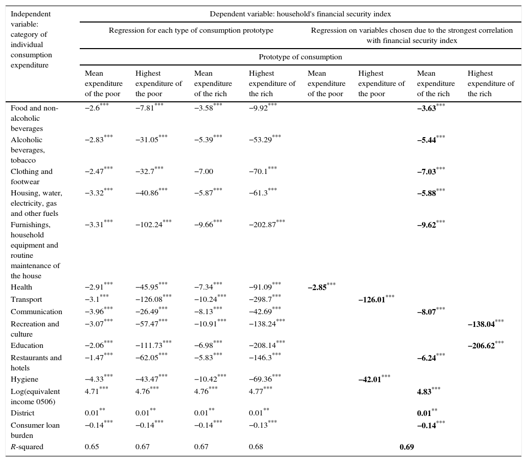
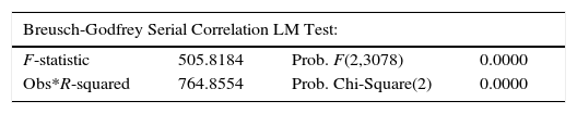
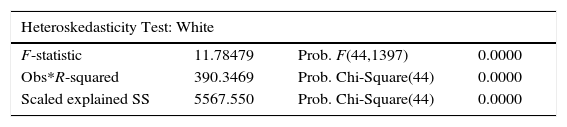
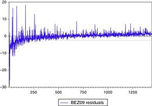
The estimation results of regressions of financial security index are presented in Tables 4–7. Under each table, there are shown: (a) a histogram and descriptive statistics of the residuals, including the Jarque–Bera statistic for testing normality; (b) a plot of residuals; (c) the Breusch-Godfrey Serial Correlation LM Test; (d) the White heteroskedasticity test. These diagnostics refer to the regression on variables chosen due to the strongest correlation with financial security index. The Jarque–Bera test suggests a lack of normality, the Breusch-Godfrey Serial Correlation LM test reveals autocorrelation and the White test shows a presence of heteroskedasticity.
Summary of the OLS (HAC standard errors and covariance) estimation results of financial security regressions for “the insecure POOR”, 2005–2006, N=4374.
| Independent variable: category of individual consumption expenditure | Dependent variable: household's financial security index | |||||||
|---|---|---|---|---|---|---|---|---|
| Regression for each type of consumption prototype | Regression on variables chosen due to the strongest correlation with financial security index | |||||||
| Prototype of consumption | ||||||||
| Mean expenditure of the poor | Highest expenditure of the poor | Mean expenditure of the rich | Highest expenditure of the rich | Mean expenditure of the poor | Highest expenditure of the poor | Mean expenditure of the rich | Highest expenditure of the rich | |
| Food and non-alcoholic beverages | −2.6*** | −7.81*** | −3.58*** | −9.92*** | −3.63*** | |||
| Alcoholic beverages, tobacco | −2.83*** | −31.05*** | −5.39*** | −53.29*** | −5.44*** | |||
| Clothing and footwear | −2.47*** | −32.7*** | −7.00 | −70.1*** | −7.03*** | |||
| Housing, water, electricity, gas and other fuels | −3.32*** | −40.86*** | −5.87*** | −61.3*** | −5.88*** | |||
| Furnishings, household equipment and routine maintenance of the house | −3.31*** | −102.24*** | −9.66*** | −202.87*** | −9.62*** | |||
| Health | −2.91*** | −45.95*** | −7.34*** | −91.09*** | −2.85*** | |||
| Transport | −3.1*** | −126.08*** | −10.24*** | −298.7*** | −126.01*** | |||
| Communication | −3.96*** | −26.49*** | −8.13*** | −42.69*** | −8.07*** | |||
| Recreation and culture | −3.07*** | −57.47*** | −10.91*** | −138.24*** | −138.04*** | |||
| Education | −2.06*** | −111.73*** | −6.98*** | −208.14*** | −206.62*** | |||
| Restaurants and hotels | −1.47*** | −62.05*** | −5.83*** | −146.3*** | −6.24*** | |||
| Hygiene | −4.33*** | −43.47*** | −10.42*** | −69.36*** | −42.01*** | |||
| Log(equivalent income 0506) | 4.71*** | 4.76*** | 4.76*** | 4.77*** | 4.83*** | |||
| District | 0.01** | 0.01** | 0.01** | 0.01** | 0.01** | |||
| Consumer loan burden | −0.14*** | −0.14*** | −0.14*** | −0.13*** | −0.14*** | |||
| R-squared | 0.65 | 0.67 | 0.67 | 0.68 | 0.69 | |||
All the regressions are estimated with the inclusion of a constant.
The bold values mean the coefficients included in the regression which is a base for the simulation which results are presented in Tables 8 and 10.
Coefficient estimates reported in the table.
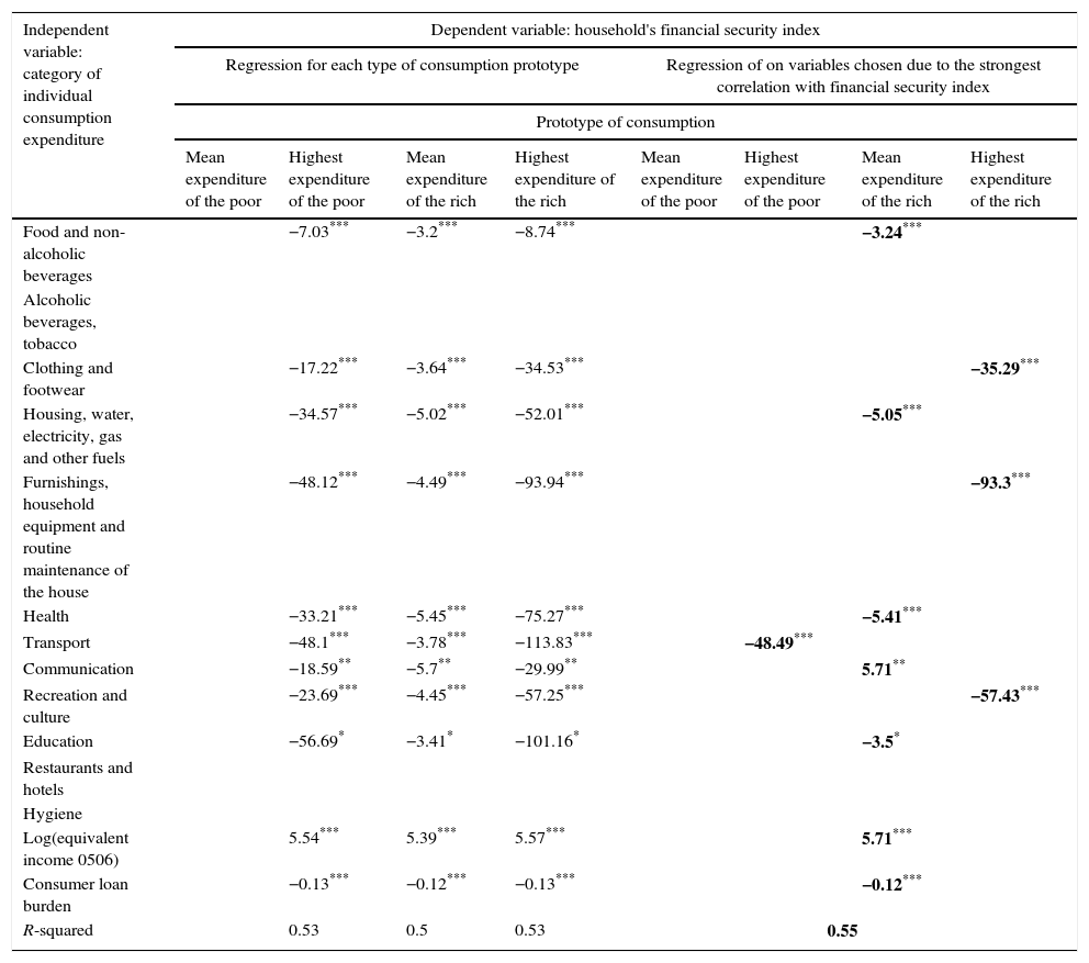
Summary of the OLS (HAC standard errors and covariance) estimation results of regressions for “the insecure RICH”, 2005–2006, N=1085.
| Independent variable: category of individual consumption expenditure | Dependent variable: household's financial security index | |||||||
|---|---|---|---|---|---|---|---|---|
| Regression for each type of consumption prototype | Regression of on variables chosen due to the strongest correlation with financial security index | |||||||
| Prototype of consumption | ||||||||
| Mean expenditure of the poor | Highest expenditure of the poor | Mean expenditure of the rich | Highest expenditure of the rich | Mean expenditure of the poor | Highest expenditure of the poor | Mean expenditure of the rich | Highest expenditure of the rich | |
| Food and non-alcoholic beverages | −7.03*** | −3.2*** | −8.74*** | −3.24*** | ||||
| Alcoholic beverages, tobacco | ||||||||
| Clothing and footwear | −17.22*** | −3.64*** | −34.53*** | −35.29*** | ||||
| Housing, water, electricity, gas and other fuels | −34.57*** | −5.02*** | −52.01*** | −5.05*** | ||||
| Furnishings, household equipment and routine maintenance of the house | −48.12*** | −4.49*** | −93.94*** | −93.3*** | ||||
| Health | −33.21*** | −5.45*** | −75.27*** | −5.41*** | ||||
| Transport | −48.1*** | −3.78*** | −113.83*** | −48.49*** | ||||
| Communication | −18.59** | −5.7** | −29.99** | 5.71** | ||||
| Recreation and culture | −23.69*** | −4.45*** | −57.25*** | −57.43*** | ||||
| Education | −56.69* | −3.41* | −101.16* | −3.5* | ||||
| Restaurants and hotels | ||||||||
| Hygiene | ||||||||
| Log(equivalent income 0506) | 5.54*** | 5.39*** | 5.57*** | 5.71*** | ||||
| Consumer loan burden | −0.13*** | −0.12*** | −0.13*** | −0.12*** | ||||
| R-squared | 0.53 | 0.5 | 0.53 | 0.55 | ||||
All the regressions are estimated with the inclusion of a constant.
The bold values mean the coefficients included in the regression which is a base for the simulation which results are presented in Tables 9 and 10.
Coefficient estimates reported in the table.
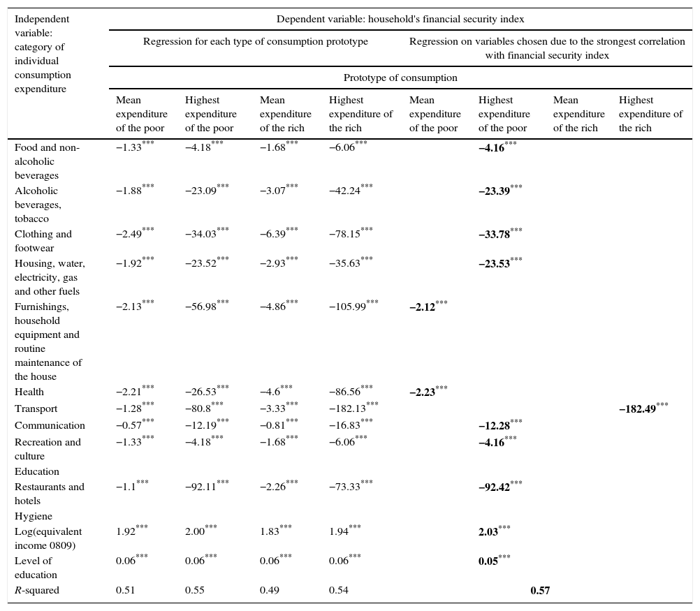
Summary of the OLS (HAC standard errors and covariance) estimation results of regressions for “the insecure POOR”, 2008–2009, N=3092.
| Independent variable: category of individual consumption expenditure | Dependent variable: household's financial security index | |||||||
|---|---|---|---|---|---|---|---|---|
| Regression for each type of consumption prototype | Regression on variables chosen due to the strongest correlation with financial security index | |||||||
| Prototype of consumption | ||||||||
| Mean expenditure of the poor | Highest expenditure of the poor | Mean expenditure of the rich | Highest expenditure of the rich | Mean expenditure of the poor | Highest expenditure of the poor | Mean expenditure of the rich | Highest expenditure of the rich | |
| Food and non-alcoholic beverages | −1.33*** | −4.18*** | −1.68*** | −6.06*** | −4.16*** | |||
| Alcoholic beverages, tobacco | −1.88*** | −23.09*** | −3.07*** | −42.24*** | −23.39*** | |||
| Clothing and footwear | −2.49*** | −34.03*** | −6.39*** | −78.15*** | −33.78*** | |||
| Housing, water, electricity, gas and other fuels | −1.92*** | −23.52*** | −2.93*** | −35.63*** | −23.53*** | |||
| Furnishings, household equipment and routine maintenance of the house | −2.13*** | −56.98*** | −4.86*** | −105.99*** | −2.12*** | |||
| Health | −2.21*** | −26.53*** | −4.6*** | −86.56*** | −2.23*** | |||
| Transport | −1.28*** | −80.8*** | −3.33*** | −182.13*** | −182.49*** | |||
| Communication | −0.57*** | −12.19*** | −0.81*** | −16.83*** | −12.28*** | |||
| Recreation and culture | −1.33*** | −4.18*** | −1.68*** | −6.06*** | −4.16*** | |||
| Education | ||||||||
| Restaurants and hotels | −1.1*** | −92.11*** | −2.26*** | −73.33*** | −92.42*** | |||
| Hygiene | ||||||||
| Log(equivalent income 0809) | 1.92*** | 2.00*** | 1.83*** | 1.94*** | 2.03*** | |||
| Level of education | 0.06*** | 0.06*** | 0.06*** | 0.06*** | 0.05*** | |||
| R-squared | 0.51 | 0.55 | 0.49 | 0.54 | 0.57 | |||
All the regressions are estimated with the inclusion of a constant.
The bold values mean the coefficients included in the regression which is a base for the simulation which results are presented in Tables 8 and 11.
Coefficient estimates reported in the table.
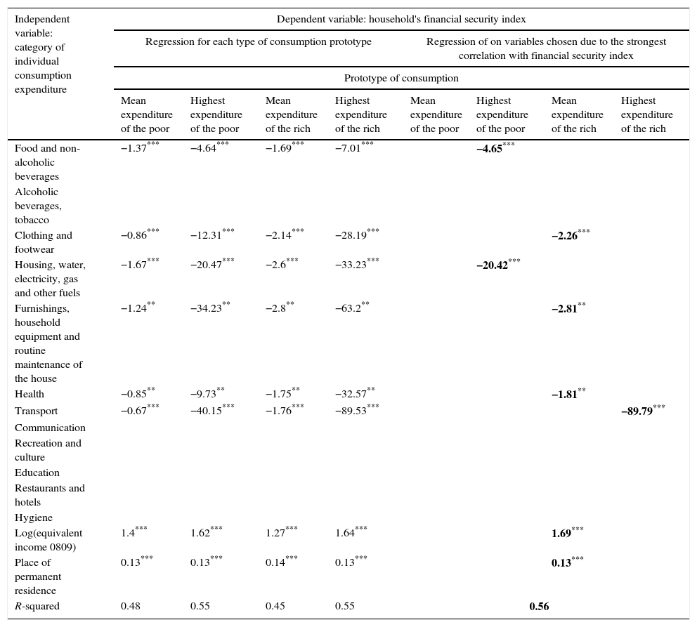
Summary of the OLS (White Heteroskedasticity) estimation results of regressions for “the insecure RICH”, 2008–2009, N=1442.
| Independent variable: category of individual consumption expenditure | Dependent variable: household's financial security index | |||||||
|---|---|---|---|---|---|---|---|---|
| Regression for each type of consumption prototype | Regression of on variables chosen due to the strongest correlation with financial security index | |||||||
| Prototype of consumption | ||||||||
| Mean expenditure of the poor | Highest expenditure of the poor | Mean expenditure of the rich | Highest expenditure of the rich | Mean expenditure of the poor | Highest expenditure of the poor | Mean expenditure of the rich | Highest expenditure of the rich | |
| Food and non-alcoholic beverages | −1.37*** | −4.64*** | −1.69*** | −7.01*** | −4.65*** | |||
| Alcoholic beverages, tobacco | ||||||||
| Clothing and footwear | −0.86*** | −12.31*** | −2.14*** | −28.19*** | −2.26*** | |||
| Housing, water, electricity, gas and other fuels | −1.67*** | −20.47*** | −2.6*** | −33.23*** | −20.42*** | |||
| Furnishings, household equipment and routine maintenance of the house | −1.24** | −34.23** | −2.8** | −63.2** | −2.81** | |||
| Health | −0.85** | −9.73** | −1.75** | −32.57** | −1.81** | |||
| Transport | −0.67*** | −40.15*** | −1.76*** | −89.53*** | −89.79*** | |||
| Communication | ||||||||
| Recreation and culture | ||||||||
| Education | ||||||||
| Restaurants and hotels | ||||||||
| Hygiene | ||||||||
| Log(equivalent income 0809) | 1.4*** | 1.62*** | 1.27*** | 1.64*** | 1.69*** | |||
| Place of permanent residence | 0.13*** | 0.13*** | 0.14*** | 0.13*** | 0.13*** | |||
| R-squared | 0.48 | 0.55 | 0.45 | 0.55 | 0.56 | |||
All the regressions are estimated with the inclusion of a constant.
The bold values mean the coefficients included in the regression which is a base for the simulation which results are presented in Tables 9 and 11.
Coefficient estimates reported in the table.
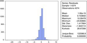
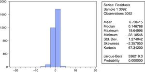
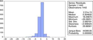
Firstly, are the residuals normally distributed? Under Tables 4–7 there are presented a histogram and descriptive statistics of the residuals, including the Jarque–Bera statistic for testing normality. If the residuals are normally distributed, the histogram should be bell-shaped and the Jarque–Bera statistic should not be significant. Jarque–Bera is a test statistic for testing whether the series is normally distributed. The test statistic measures the difference of the skewness and kurtosis of the series with those from the normal distribution. The reported Probability is the probability that a Jarque–Bera statistic exceeds (in absolute value) the observed value under the null hypothesis. For each regression presented in Tables 4–7 the zero probability value leads to the rejection of the null hypothesis of a normal distribution.
This conclusion seems to be doubtful because, in the presence of outliers, the power of the Jarque–Bera test is low. If the distribution is disturbed by outliers (data points with really big positive or negative residuals) a value of the test statistic becomes huge in comparison to the critical value. The test suggests that the distribution considerably departs from the normal one. However, a decision to reject the null hypothesis of a normal distribution is influenced by outliers. In such a case, one should take into account that tails of a distribution are the most important issue in carrying out statistical inference. If a distribution in its ends is close to the assumed distribution, the factual values of statistical tests will be equal to the assumed values. It is much less important for statistical inference how the distribution looks in its remaining part.
Each of the residual distributions shown in the boxes under Tables 4–7 is influenced by outliers (compare mean and maximum, minimum values in the descriptive statistics). It results in the huge values of Jarque–Bera statistics. However, the tails of these distributions are rather close to the normal distribution (see the histograms in the boxes). It allows to assumed that the residual distribution is normal for each regression shown in Tables 4–7 (taking into account that applying the M-method has not improved the values of skewness and kurtosis).2
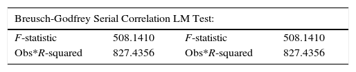
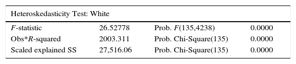
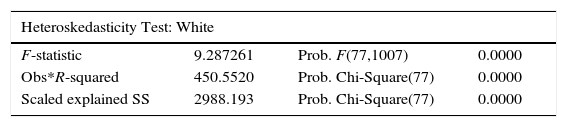
Secondly, the Breusch-Godfrey LM test (see point c below each of Tables 4–7) shows autocorrelation. Neighboring error terms are correlated because the values of the dependent variable (the financial security index) are ordered from maximum to minimum. The next problem refers to heteroskedasticity. Have the error terms for all observations a common variance (are they homoskedastic) or a varying variance (are the error terms heteroskedastic)? One of the statistical assumptions underneath ordinary least squares is that the error terms for all observations have a common variance. Based on the White test statistics, the null of homoskedascity is rejected (see the point d under each of Tables 4–7). This means that the error term in each regression is heteroskedastic and standard errors must be adjusted.
The common approach to dealing with both autocorrelation of unknown form and heteroskedasticity is to use the HAC Consistent Covariance (Newey-West). An idea is to stick with least squares estimation, but to adjust the standard errors for heteroskedasticity and autocorrelation of unknown form. In Tables 4–7 the summary of the OLS (HAC Consistent Covariance (Newey-West)) estimation results of financial security regressions are presented.
For purpose of comparison the full results with unadjusted standard errors (the OLS estimation) and the results with adjusted standard errors (the OLS – HAC Consistent Covariance (Newey-West)) are reported in Appendix. As expected, the estimated coefficient values do not change. But the adjusted standard errors (and associated t-statistics) – Tables Ib, IIb, IIIb, IVb in Appendix – are different from the original regressions – Tables Ia, IIa, IIIa, IVa – suggesting that autocorrelation and heteroskedasticity are present and should be corrected (what is done).
Returning to the OLS (HAC Consistent Covariance (Newey-West)) estimation results of financial security regressions – Tables 4–7, (and Tables Ib, IIb, IIIb, IVb in Appendix) – a majority of coefficient estimates on independent variables are significant at the 1% level, few ones at the 5% level and only one at the 10% level (p=0.0777, Table IIb in Appendix).
Diagnostic tests for the regression on variables chosen due to the strongest correlation with the financial security index – “the insecure POOR”, 2005–2006 (Table 4):
- a)
the histogram with the descriptive statistics including the Jarque–Bera statistic for testing normality
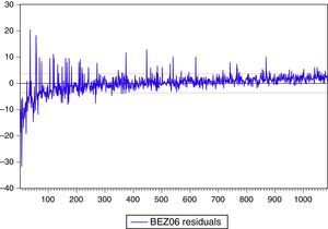
- b)
the plot of residuals for the financial security regression, the sample of “The Insecure POOR”, 2005–2006 (The symbol “BEZ06” means the financial security index in 2006)
- c)
The Breusch-Godfrey Serial Correlation LM Test
- d)
the White heteroskedasticity test
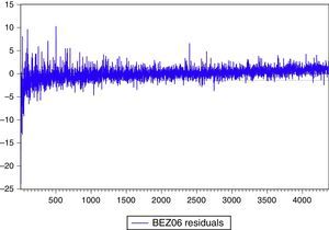
Diagnostic tests for the regression on variables chosen due to the strongest correlation with the financial security index – “the insecure RICH”, 2005–2006 (Table 5):
- a)
the histogram with the descriptive statistics including the Jarque–Bera statistic for testing normality
- b)
the plot of residuals for the financial security regression, the sample of “the insecure RICH”, 2005–2006 (The symbol “BEZ06” means the financial security index in 2006)
- c)
The Breusch-Godfrey Serial Correlation LM Test
- d)
the White heteroskedasticity test
Diagnostic tests for the regression on variables chosen due to the strongest correlation with the financial security index – “the insecure POOR”, 2008–2009 (Table 6):
- a)
the histogram with the descriptive statistics including the Jarque–Bera statistic for testing normality
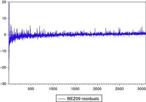
- b)
the plot of residuals for the financial security regression, the sample of “The Insecure POOR”, 2008–20069 (The symbol “BEZ09” means the financial security index in 2009)
- c)
The Breusch-Godfrey Serial Correlation LM Test
- d)
the White heteroskedasticity test
Diagnostic tests for the regression on variables chosen due to the strongest correlation with the financial security index – “the insecure RICH”, 2008–2009 (Table 7):
- a)
the histogram with the descriptive statistics including the Jarque–Bera statistic for testing normality
- b)
the plot of residuals for the financial security regression, the sample of “the insecure RICH”, 2008–20069 (The symbol “BEZ09” means the financial security index in 2009)
- c)
The Breusch-Godfrey Serial Correlation LM Test
- d)
the White heteroskedasticity test
The coefficient estimates on variables in the financial security index regressions are used to carry out the simple simulation of the type: “what if”. “Variables” mean the 2-year sum of weighted distances between the household's expenses on each category of consumption expenditure and the given prototype of consumption. The simulation is aimed at estimating to what extent the household's financial security could decline as the result of one-standard-deviation increase in the category of consumption expenditure The exercise allows to rank the expenses on particular categories of consumer goods and services taking into account their influence on financial security of households. The calculation is based on the coefficient estimates in the regression and it runs as follows: One-standard-deviation increase in the category of consumption expenditure=parameter of variable×mean standard deviation of a variable. The percentage decline in financial security is calculated under the assumption that the value of a chosen variable increases by one standard deviation, keeping remaining variables in the regression constant at their previous levels for a given household. The percentage decline in financial security due to the increase in a given variable is the average ratio of one-standard-deviation increase in this variable (it means the increase in a given category of consumption expenditure) to existing level of the household's financial security index (the sum of the declines in household's financial security index=100%). The results of simulation are presented in Tables 8–11.
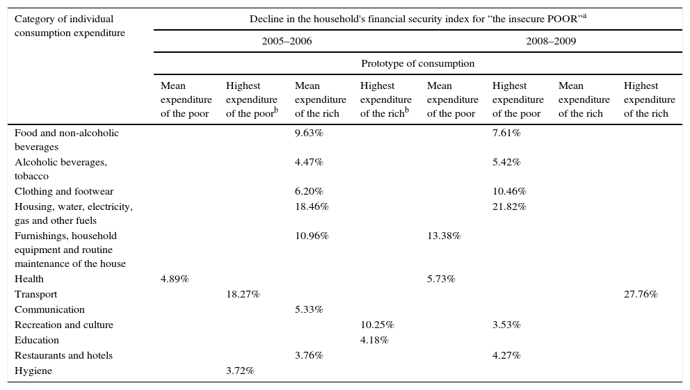
The results of simulation for “the insecure POOR”, 2005–2006 and 2008–2009 – the decline in the household's financial security index resulted from one-standard-deviation increase in the category of consumption expenditure (the sum of the declines in household's financial security index=100%).
| Category of individual consumption expenditure | Decline in the household's financial security index for “the insecure POOR”a | |||||||
|---|---|---|---|---|---|---|---|---|
| 2005–2006 | 2008–2009 | |||||||
| Prototype of consumption | ||||||||
| Mean expenditure of the poor | Highest expenditure of the poorb | Mean expenditure of the rich | Highest expenditure of the richb | Mean expenditure of the poor | Highest expenditure of the poor | Mean expenditure of the rich | Highest expenditure of the rich | |
| Food and non-alcoholic beverages | 9.63% | 7.61% | ||||||
| Alcoholic beverages, tobacco | 4.47% | 5.42% | ||||||
| Clothing and footwear | 6.20% | 10.46% | ||||||
| Housing, water, electricity, gas and other fuels | 18.46% | 21.82% | ||||||
| Furnishings, household equipment and routine maintenance of the house | 10.96% | 13.38% | ||||||
| Health | 4.89% | 5.73% | ||||||
| Transport | 18.27% | 27.76% | ||||||
| Communication | 5.33% | |||||||
| Recreation and culture | 10.25% | 3.53% | ||||||
| Education | 4.18% | |||||||
| Restaurants and hotels | 3.76% | 4.27% | ||||||
| Hygiene | 3.72% | |||||||
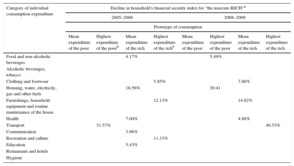
The results of simulation for “the insecure RICH”, 2005–2006 and 2008–2009 – the decline in the household's financial security index as a result of one-standard-deviation increase in a category of consumption expenditure (the sum of the declines in household's financial security index=100%).
| Category of individual consumption expenditure | Decline in household's financial security index for “the insecure RICH”a | |||||||
|---|---|---|---|---|---|---|---|---|
| 2005–2006 | 2008–2009 | |||||||
| Prototype of consumption | ||||||||
| Mean expenditure of the poor | Highest expenditure of the poorb | Mean expenditure of the rich | Highest expenditure of the richb | Mean expenditure of the poor | Highest expenditure of the poor | Mean expenditure of the rich | Highest expenditure of the rich | |
| Food and non-alcoholic beverages | 4.17% | 5.49% | ||||||
| Alcoholic beverages, tobacco | ||||||||
| Clothing and footwear | 5.95% | 7.86% | ||||||
| Housing, water, electricity, gas and other fuels | 18.56% | 20.41 | ||||||
| Furnishings, household equipment and routine maintenance of the house | 12.13% | 14.82% | ||||||
| Health | 7.00% | 4.88% | ||||||
| Transport | 31.57% | 46.53% | ||||||
| Communication | 3.86% | |||||||
| Recreation and culture | 11.33% | |||||||
| Education | 5.43% | |||||||
| Restaurants and hotels | ||||||||
| Hygiene | ||||||||
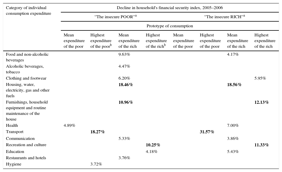
The results of simulation for “the insecure POOR” and for “the insecure RICH”, 2005–2006 – the decline in the household's financial security index as a result of one-standard-deviation increase in a category of consumption expenditure (the sum of the declines in household's financial security index=100%).
| Category of individual consumption expenditure | Decline in household's financial security index, 2005–2006 | |||||||
|---|---|---|---|---|---|---|---|---|
| “The insecure POOR”a | “The insecure RICH”a | |||||||
| Prototype of consumption | ||||||||
| Mean expenditure of the poor | Highest expenditure of the poorb | Mean expenditure of the rich | Highest expenditure of the richb | Mean expenditure of the poor | Highest expenditure of the poor | Mean expenditure of the rich | Highest expenditure of the rich | |
| Food and non-alcoholic beverages | 9.63% | 4.17% | ||||||
| Alcoholic beverages, tobacco | 4.47% | |||||||
| Clothing and footwear | 6.20% | 5.95% | ||||||
| Housing, water, electricity, gas and other fuels | 18.46% | 18.56% | ||||||
| Furnishings, household equipment and routine maintenance of the house | 10.96% | 12.13% | ||||||
| Health | 4.89% | 7.00% | ||||||
| Transport | 18.27% | 31.57% | ||||||
| Communication | 5.33% | 3.86% | ||||||
| Recreation and culture | 10.25% | 11.33% | ||||||
| Education | 4.18% | 5.43% | ||||||
| Restaurants and hotels | 3.76% | |||||||
| Hygiene | 3.72% | |||||||
The bold value means the highest decline in the household's financial security index as a result of one-standard-deviation increase in a given category of consumption expenditure.
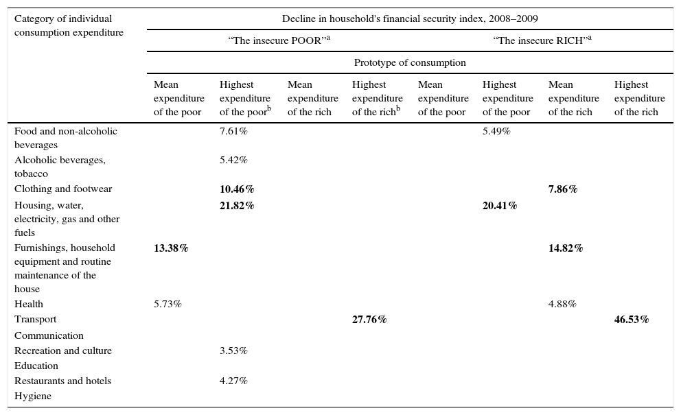
The results of simulation for “the insecure POOR” and for “the insecure RICH”, 2008–2009 – the decline in the household's financial security index as a result of one-standard-deviation increase in a category of consumption expenditure (the sum of the declines in household's financial security index=100%).
| Category of individual consumption expenditure | Decline in household's financial security index, 2008–2009 | |||||||
|---|---|---|---|---|---|---|---|---|
| “The insecure POOR”a | “The insecure RICH”a | |||||||
| Prototype of consumption | ||||||||
| Mean expenditure of the poor | Highest expenditure of the poorb | Mean expenditure of the rich | Highest expenditure of the richb | Mean expenditure of the poor | Highest expenditure of the poor | Mean expenditure of the rich | Highest expenditure of the rich | |
| Food and non-alcoholic beverages | 7.61% | 5.49% | ||||||
| Alcoholic beverages, tobacco | 5.42% | |||||||
| Clothing and footwear | 10.46% | 7.86% | ||||||
| Housing, water, electricity, gas and other fuels | 21.82% | 20.41% | ||||||
| Furnishings, household equipment and routine maintenance of the house | 13.38% | 14.82% | ||||||
| Health | 5.73% | 4.88% | ||||||
| Transport | 27.76% | 46.53% | ||||||
| Communication | ||||||||
| Recreation and culture | 3.53% | |||||||
| Education | ||||||||
| Restaurants and hotels | 4.27% | |||||||
| Hygiene | ||||||||
The bold value means the highest decline in the household's financial security index as a result of one-standard-deviation increase in a given category of consumption expenditure.
The estimations of financial security regressions show that status-oriented consumption (reflected by the distances of the household's consumption expenditure from the consumption prototypes) is a statistically significant cause that threatens financial security of both groups of households: the rich and the poor (see Tables 4–7). Purchasing for display keeps its dominant influence on financial insecurity when several control variables have been included in the regressions. Among these controls only income has been statistically significant in both periods, while consumer loan burden contributed to financial insecurity a little bit only in the first period, 2005–2006, and it was replaced in 2008–2009 by the educational level with reference to the insecure poor (higher educational level higher financial security) and by the place of permanent residence considering the insecure rich (larger town as a place of residence higher financial security). Other controls like, age, the family size, a source of income (hired work or self-employment), housing loan burden were statistically insignificant in both periods.
The results of simulationTables 8–11 present the simulation results, it means the decline in the household's financial security index (or the increase in financial insecurity) resulted from one-standard-deviation increase in the category of consumption expenditure (the sum of the declines in the household's financial security index=100%) for two groups, the insecure poor and the insecure rich, as well as in two periods: 2005–2006 and 2008–2009. These results allow:
- -
to rank expenditures on the consumption categories taking into account their influences on households’ financial insecurity;
- -
to show the changes in the relevance of consumption expenditures on particular categories over time;
- -
to find out the similarities and differences between the insecure poor and the insecure rich;
- -
to reveal the dominant prototypes of consumption;
- -
to point at status goods.
Tables 12 and 13 show the rankings of consumption expenses considering their influences on households’ financial insecurity.
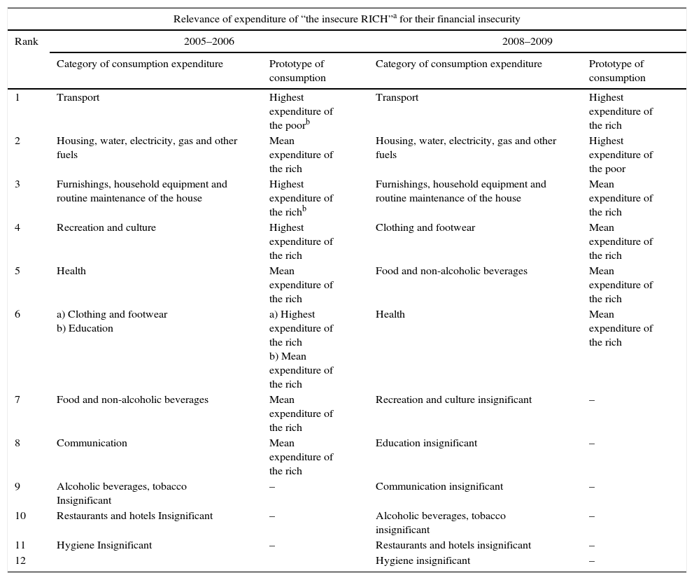
Ranking of consumption expenses considering their influences on households’ financial insecurity – the insecure RICH, 2005–2006 and 2008–2009.
| Relevance of expenditure of “the insecure RICH”a for their financial insecurity | ||||
|---|---|---|---|---|
| Rank | 2005–2006 | 2008–2009 | ||
| Category of consumption expenditure | Prototype of consumption | Category of consumption expenditure | Prototype of consumption | |
| 1 | Transport | Highest expenditure of the poorb | Transport | Highest expenditure of the rich |
| 2 | Housing, water, electricity, gas and other fuels | Mean expenditure of the rich | Housing, water, electricity, gas and other fuels | Highest expenditure of the poor |
| 3 | Furnishings, household equipment and routine maintenance of the house | Highest expenditure of the richb | Furnishings, household equipment and routine maintenance of the house | Mean expenditure of the rich |
| 4 | Recreation and culture | Highest expenditure of the rich | Clothing and footwear | Mean expenditure of the rich |
| 5 | Health | Mean expenditure of the rich | Food and non-alcoholic beverages | Mean expenditure of the rich |
| 6 | a) Clothing and footwear b) Education | a) Highest expenditure of the rich b) Mean expenditure of the rich | Health | Mean expenditure of the rich |
| 7 | Food and non-alcoholic beverages | Mean expenditure of the rich | Recreation and culture insignificant | – |
| 8 | Communication | Mean expenditure of the rich | Education insignificant | – |
| 9 | Alcoholic beverages, tobacco Insignificant | – | Communication insignificant | – |
| 10 | Restaurants and hotels Insignificant | – | Alcoholic beverages, tobacco insignificant | – |
| 11 | Hygiene Insignificant | – | Restaurants and hotels insignificant | – |
| 12 | Hygiene insignificant | – | ||
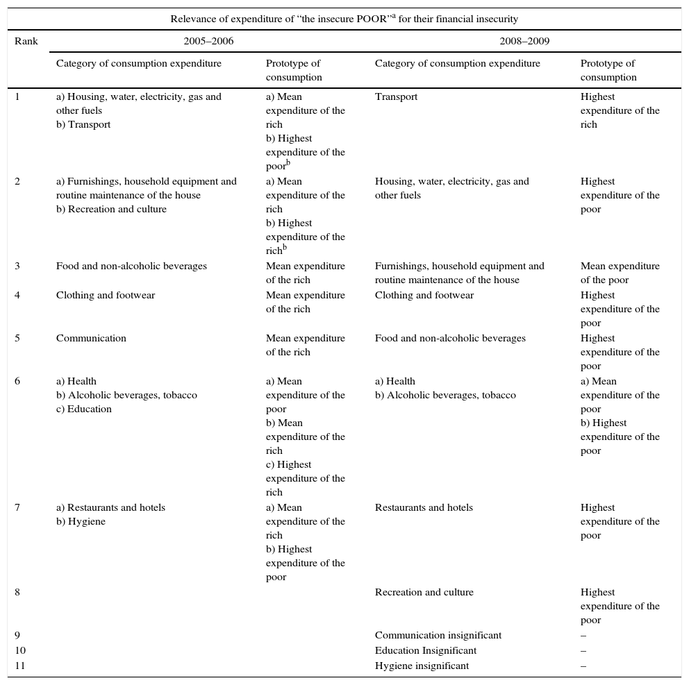
Ranking of consumption expenses considering their influences on households’ financial insecurity – the insecure POOR, 2005–2006 and 2008–2009.
| Relevance of expenditure of “the insecure POOR”a for their financial insecurity | ||||
|---|---|---|---|---|
| Rank | 2005–2006 | 2008–2009 | ||
| Category of consumption expenditure | Prototype of consumption | Category of consumption expenditure | Prototype of consumption | |
| 1 | a) Housing, water, electricity, gas and other fuels b) Transport | a) Mean expenditure of the rich b) Highest expenditure of the poorb | Transport | Highest expenditure of the rich |
| 2 | a) Furnishings, household equipment and routine maintenance of the house b) Recreation and culture | a) Mean expenditure of the rich b) Highest expenditure of the richb | Housing, water, electricity, gas and other fuels | Highest expenditure of the poor |
| 3 | Food and non-alcoholic beverages | Mean expenditure of the rich | Furnishings, household equipment and routine maintenance of the house | Mean expenditure of the poor |
| 4 | Clothing and footwear | Mean expenditure of the rich | Clothing and footwear | Highest expenditure of the poor |
| 5 | Communication | Mean expenditure of the rich | Food and non-alcoholic beverages | Highest expenditure of the poor |
| 6 | a) Health b) Alcoholic beverages, tobacco c) Education | a) Mean expenditure of the poor b) Mean expenditure of the rich c) Highest expenditure of the rich | a) Health b) Alcoholic beverages, tobacco | a) Mean expenditure of the poor b) Highest expenditure of the poor |
| 7 | a) Restaurants and hotels b) Hygiene | a) Mean expenditure of the rich b) Highest expenditure of the poor | Restaurants and hotels | Highest expenditure of the poor |
| 8 | Recreation and culture | Highest expenditure of the poor | ||
| 9 | Communication insignificant | – | ||
| 10 | Education Insignificant | – | ||
| 11 | Hygiene insignificant | – | ||
With reference to financial insecurity experienced by the rich, expenses on the same categories of consumer goods and services – (1) transport, (2) housing and (3) furnishings plus household equipment–have three first ranks both in 2005–2006 as well as 2008–2009 (see Table 12). Expenses on these goods and services have generated to largest extent financial insecurity among members of the insecure rich group.
There are two visible changes in the ranking over time. First, expenses on some categories completely lost their influences on financial insecurity of the rich in 2008–2009: first of all expenses on recreation and culture which had relatively high, fourth rank in 2005–2006, moreover, expenses on education and communication. Second, expenses on clothing and footwear as well as on food, what is specially interesting considering the rich, improved their ranks in 2008–2009, it means that expenses on these goods much stronger generated financial insecurity of the rich than three years earlier.
The relevance of expenses on particular categories of consumption expenditure for financial insecurity experienced by the poor is better recognized in 2008–2009 than 2005–2006 (see Table 13). The differences in the influences of expenses that have two first ranks in 2005–2006 are rather small. In 2008–2009 the ranking became transparent. Expenses on (1) transport, (2) housing, and (3) furnishings plus household equipment, were responsible for financial insecurity across members of the poor group in 2008–2009. The influence of expenses on recreation and culture has become much smaller (the most visible change over time), while expenses on communication, education and hygiene completely lost their impact on financial insecurity of the poor in 2008–2009.
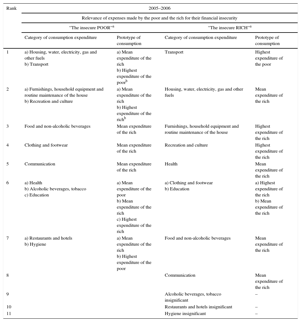
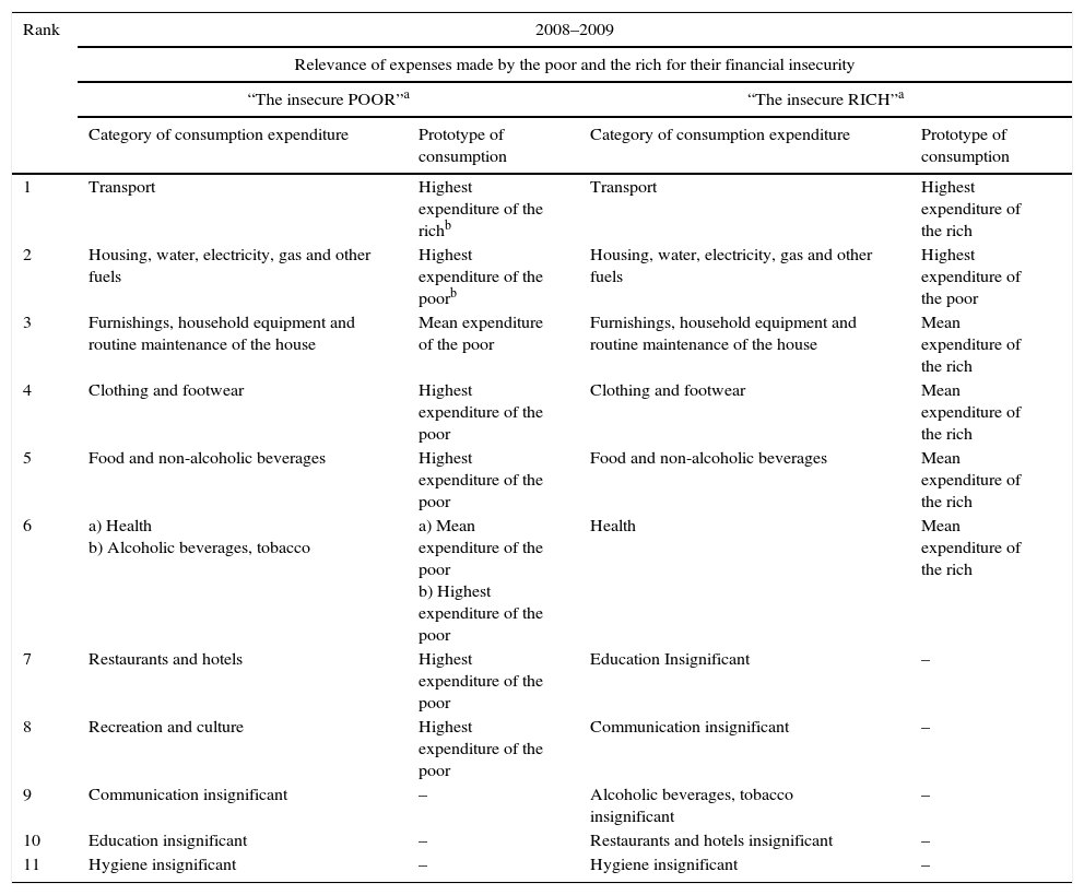
The similarities and differences between the insecure poor and the insecure richTables 14 and 15 allow to compare the relevance of the categories of consumption expenditure for financial insecurity between the poor and the rich. There are four main similarities The most visible one is that the same categories of consumer goods and services have the first three ranks for both groups of households in both periods. There are expenses on: (1) transport, (2) housing, and (3) furnishings plus household equipment. Furthermore, the impact of expenses on recreation and culture, which generated to considerable extent financial insecurity of both groups in 2005–2006, became much weaker (for the poor) or statistically insignificant (for the poor) in 2008–2009. Expenses on clothing and footwear improved its rank in 2008–2009. In general, there is some convergence in the influence of consumer goods and services categories on financial insecurity of both groups. In 2005–2006 only the first three ranks were occupied by the same categories while in 2008–2009 the rankings were similar up to the sixth position.
Ranking of consumption expenses considering their influences on households’ financial insecurity – the insecure RICH and the insecure POOR, 2005–2006.
| Rank | 2005–2006 | |||
|---|---|---|---|---|
| Relevance of expenses made by the poor and the rich for their financial insecurity | ||||
| “The insecure POOR”a | “The insecure RICH”a | |||
| Category of consumption expenditure | Prototype of consumption | Category of consumption expenditure | Prototype of consumption | |
| 1 | a) Housing, water, electricity, gas and other fuels b) Transport | a) Mean expenditure of the rich b) Highest expenditure of the poorb | Transport | Highest expenditure of the poor |
| 2 | a) Furnishings, household equipment and routine maintenance of the house b) Recreation and culture | a) Mean expenditure of the rich b) Highest expenditure of the richb | Housing, water, electricity, gas and other fuels | Mean expenditure of the rich |
| 3 | Food and non-alcoholic beverages | Mean expenditure of the rich | Furnishings, household equipment and routine maintenance of the house | Highest expenditure of the rich |
| 4 | Clothing and footwear | Mean expenditure of the rich | Recreation and culture | Highest expenditure of the rich |
| 5 | Communication | Mean expenditure of the rich | Health | Mean expenditure of the rich |
| 6 | a) Health b) Alcoholic beverages, tobacco c) Education | a) Mean expenditure of the poor b) Mean expenditure of the rich c) Highest expenditure of the rich | a) Clothing and footwear b) Education | a) Highest expenditure of the rich b) Mean expenditure of the rich |
| 7 | a) Restaurants and hotels b) Hygiene | a) Mean expenditure of the rich b) Highest expenditure of the poor | Food and non-alcoholic beverages | Mean expenditure of the rich |
| 8 | Communication | Mean expenditure of the rich | ||
| 9 | Alcoholic beverages, tobacco insignificant | – | ||
| 10 | Restaurants and hotels insignificant | – | ||
| 11 | Hygiene insignificant | – | ||
Ranking of consumption expenses considering their influences on households’ financial insecurity –the insecure RICH and the insecure POOR, 2008–2009.
| Rank | 2008–2009 | |||
|---|---|---|---|---|
| Relevance of expenses made by the poor and the rich for their financial insecurity | ||||
| “The insecure POOR”a | “The insecure RICH”a | |||
| Category of consumption expenditure | Prototype of consumption | Category of consumption expenditure | Prototype of consumption | |
| 1 | Transport | Highest expenditure of the richb | Transport | Highest expenditure of the rich |
| 2 | Housing, water, electricity, gas and other fuels | Highest expenditure of the poorb | Housing, water, electricity, gas and other fuels | Highest expenditure of the poor |
| 3 | Furnishings, household equipment and routine maintenance of the house | Mean expenditure of the poor | Furnishings, household equipment and routine maintenance of the house | Mean expenditure of the rich |
| 4 | Clothing and footwear | Highest expenditure of the poor | Clothing and footwear | Mean expenditure of the rich |
| 5 | Food and non-alcoholic beverages | Highest expenditure of the poor | Food and non-alcoholic beverages | Mean expenditure of the rich |
| 6 | a) Health b) Alcoholic beverages, tobacco | a) Mean expenditure of the poor b) Highest expenditure of the poor | Health | Mean expenditure of the rich |
| 7 | Restaurants and hotels | Highest expenditure of the poor | Education Insignificant | – |
| 8 | Recreation and culture | Highest expenditure of the poor | Communication insignificant | – |
| 9 | Communication insignificant | – | Alcoholic beverages, tobacco insignificant | – |
| 10 | Education insignificant | – | Restaurants and hotels insignificant | – |
| 11 | Hygiene insignificant | – | Hygiene insignificant | – |
There are some differences. First, expenses on larger number of consumer goods and services categories have generated financial insecurity of the poor than of the rich. Second, expenses on such categories like: alcoholic beverages, tobacco; restaurants and hotels; hygiene, were statistically insignificant in explaining financial insecurity of the rich in both periods while they influenced financial position of the poor at least in one period. Third, expenses on food kept its position in the ranking for the insecure poor in both periods while the influence of food expenses on financial insecurity of the rich increased in 2008–2009 in comparison to 2005–2006.
The dominant prototypes of consumptionDisplay consumption is influenced by Veblen, snob and bandwagon effects, (Liebenstein, 1950). Veblen effects are recognized when individuals use product price as a means of ostentatiously displaying wealth; snob effects stimulate consumers to buy an item because of its relative scarcity value; and bandwagon effects intend people to purchase goods and services in order to be identified with a particular social group. Cultural traditions and social values have always shaped the pattern of status-directed consumption (Mason, 1993). Display consumption, however, is now heavily influenced by multinational companies and television that create “international” culture and commercially-sponsored value systems.
The findings suggest some patterns of consumption. In the period of 2005–2006 mean expenditure of the rich was the dominant prototype of consumption for the insecure poor (see Table 9). There were only three exceptions to it: the highest expenses of the rich for recreation, the highest expenses of the poor for transport and the mean expenses of the poor for health. In general, consumer behavior of the insecure poor was shaped by liking for the rich and the need to create the impression of attachment to the group with higher consumption. Only prototype of expenses on transport reveals the need to improve the household's self-image by having consumption at the highest level in own group.
In 2008–2009 after four years of dynamic growth and the increases in incomes of all groups, the highest expenditure of the poor became the prototype of consumption for the insecure poor (it is worth to remember at this moment that the highest expenditure of the poor is much higher than mean expenditure of the rich). Consumer behavior of the insecure poor was influenced by the need to improve the household's self-image by approaching own consumption to the highest level recognized as possible to meet by the poor.
Consumer behavior of the insecure rich has been shaped mostly by the need to be distinguishable inside of own income-group by having consumption at higher level than the own-group average. The dominant prototype of consumption is mean expenditure of the rich in both periods. Liking for the highest expenses has been shown with reference to a few categories of goods and services.
The tendency in the dominant prototype of consumption toward higher and higher expenses can strongly deepen financial insecurity of the poor if the second wave of financial crisis visibly declines economic activity in Poland. The question is still open how fast the insecure poor as well as the insecure rich will able to change their consumer behavior in a response to slower growth. When 50% households has not be able to generate savings over two years, job loss could threaten standards of life.
The status goodsThe findings point at a car as the main status good accepted both by the poor and the rich. The desire of having a car has intended many households to acquire expenditure beyond their means. Spending on a car has been seen by conspicuous consumers as means of attaining or maintaining their social status. A car plays its role, as a status good, very well because it is a good consumed publicly and it can be seen and evaluated by “relevant others”.
Housing is the second symbol of status-oriented consumption. The size of a home or flat, its location, the standard of facilities matter for improving the household's image. People want to live like the reference group enjoying the highest spending on housing.
A trend toward the higher expenditure on cars and housing results in the inability to save funds by quite considerable fraction of households in both groups: the rich and the poor.
Furnishings and household equipment are the third status good. What is interesting that the prototypes of consumption for both the rich and the poor have shifted from the highest expenses to mean expenses inside own income-group. Probably, the character of these goods is responsible for such a change. Furnishings and household equipment are consumed privately, and it is enough to be better than friends and relatives to be distinguishable. It is not necessary to compare themselves to people spending a lot on these goods.
The research has not been aimed at distinguishing Veblen, snob and bandwagon effects. It is difficult to evaluate causes for which clothing and footwear is the fourth status good for both the rich and the poor. Designer clothes can be bought for Veblen and snob motives as well as for bandwagon effects. However, the relatively high position of clothes in status consumption may signal the growing importance of personal display. Probably the shift of food to the fifth position in the ranking of status goods for the rich suggests also expressing conspicuous consumption to larger extent through personal lifestyle. But on the other side the opposite argument can be drawn from the fact that recreation has lost its relevance, as a status good, when prices of touristic services have gone visibly down as a typical Veblen effect predicts.
It seems that up to now in Poland display consumption is expressed through conspicuous expenditures on cars and homes rather than through style and taste. In this sense consumer behavior in Poland is more similar to conspicuous consumption in the United States than in France, for example.
Poland shares the consumption patterns with other transition countries in Europe and Central Asia.
Consumption patterns in Central and Eastern European Countries (CEECs) have been shaped by two factors:
- 1)
bandwagon purchasing, driven by the pervasive influence of multinational corporations and of global communication networks – as a consequence interest in both conspicuous consumption and in bandwagon effects has created a substantial demand for snob products among those consumers for whom status consumption has been used as an expression of individualism and personal distinction. (Mason, 1993)
- 2)
the heritage from the Communist rule – it is characterized by “the economy of permanent shortage” – household consumption was very restricted and created an enormous hunger for goods and western lifestyle (Fammler, 2011, p. 19).
To reach west European economic wealth has been a major policy goal in all CEE countries since their shift to a market economy. Therefore the hunger for consumer goods and western lifestyle at CEEC is easy to understand.
Mroz (2010, p. 14) emphasizes on the pervasive influence of multinational corporations and of global communication networks: “After decades of ascetic consumption, the Polish consumers will not be easily persuaded to exercise self-restraint, the more so as the world of industry, commerce, media and advertisement sends them compelling signals with enticement to increased consumption”.
The structure of household expenditure has also changed and adapted to the western pattern: when the total available household budget is growing, the percentage spent on satisfying basic needs is decreasing. More and more money is spent for transport, recreation and housing. This stands for all CEE region, with a slightly different time scale and break down of household structure (Fammler, 2011, Graph 3, p. 9). Zilahy and Zsóka (2012, Figure 15, p. 14) call attention to an interesting indicator of consumption, the purchasing and registration of private cars. The recession (2008–2009) spitted both CEE and other, more developed countries: Hungary, Estonia and Slovenia (CEE) as well as Spain, Finland and the U.K. (developed) showed a marked decrease in registration, while other countries (e.g. Czech Republic, Slovak Republic, Austria and France) were able to grow in this respect.
The changes in consumption patterns observed in Southeast Europe, Caucasus and Central Asia between 1995–2005 were similar to the changes in CEECs (report, jointly prepared by the United Nations Environment Programme (UNEP) and the European Environment Agency (EEA), 2007) The additional income was used increasingly on housing and utilities, transport and communication, home appliances and recreation.
Household consumption patterns varied widely across countries in the period of 1995–2005. In the lower-income countries of Central Asia and the Caucasus, greater proportions of household expenditures were set aside for food. This was most pronounced in Tajikistan and Armenia where food represented 64% and 57% of average household expenditures, respectively. In Tajikistan, despite increases in incomes since the mid-1990s, there remained little surplus for non-essentials in the average household. At the other extreme, Croatia, which had the highest household expenditure per capita across the regions, used the smallest proportion on food (33%) and the highest on transport and communication and recreation, culture and healthcare.
Since the 1990s, European preoccupation with the environment and with the need to protect and preserve natural resources has been still continued to grow. It has become increasingly counterproductive to indulge in wasteful expenditure, particularly when the waste had strong environmental overtones and has been seen to diminish the overall quality of life.
Nowadays financial incentives for “smart consumption” are still largely missing in CEE countries. Environmental goods and principles, e.g. energy efficiency of housing, have been only introduced to the market after the energy shortage and the stricter EU legislative frame made members states act. However, as soon as the cost burden lowers, people are ready to consume much more environmental friendly goods (Fammler, 2011, p. 19).
ConclusionsThe findings offer empirical evidence for the relevance of consumer behavior for financial security of households in Poland. Considerable part of households expresses the identity through conspicuous consumption. The need to be distinguishable inside own income-group shapes the consumption prototype of the insecure rich while a desire to improve self-image by approaching own consumption to the highest expenses seems to be the dominant consumer behavior rather for the insecure poor.
Both groups of households accept the same ranking of status goods: a car on the first position, next homes (housing and equipment) and clothe on the third place. Status-oriented consumption creates life beyond means and pushes even relatively rich households toward financial insecurity. The budget constrain is beaten by the need to improve social status.
Explanation for the variables names in tables in Appendix:
BEZ06; BEZ09 – financial security index in 2006 and 2009, respectively
The name of each main independent variable covers:
The symbols of consumption expenditure categories are as follows:
ZYW – Food and non-alcoholic beverages
AL – Alcoholic beverages, tobacco
OD – Clothing and footwear
UZM – Housing, water, electricity, gas and other fuels
WYM – Furnishings, household equipment and routine maintenance of the house
ZD – health
TR – Transport
LA – Communication
RE – Recreation and culture
ED – Education
RH – Restaurants and hotels
HI – Hygiene
The symbols of the consumption prototypes are as follows:
Names of controls are as follows:
DOCHEK56; DOCHEK89 – a sum of equivalent income in two years (in 2005 and 2006; 2008 and 2009, respectively)
WO – district
KRE – consumer loan of burden
WYKSZ – level of education
KLM – place of permanent residence
The OLS estimation results of financial security regressions for “the insecure POOR”, 2005–2006, N=4374.
| Dependent variable: BEZ06 |
| Method: least squares |
| Sample: 1 4374 |
| Included observations: 4374 |
| Coefficient | Std. Error | t-Statistic | Prob. | |
|---|---|---|---|---|
| C | −30.35643 | 0.586007 | −51.80213 | 0.0000 |
| ZYWRM | −3.625362 | 0.156623 | −23.14709 | 0.0000 |
| ALRM | −5.444067 | 0.449334 | −12.11585 | 0.0000 |
| ODRM | −7.030983 | 0.458682 | −15.32867 | 0.0000 |
| UZMRM | −5.884140 | 0.122813 | −47.91138 | 0.0000 |
| WYMRM | −9.617382 | 0.329135 | −29.22020 | 0.0000 |
| ZDPM | −2.853154 | 0.227384 | −12.54773 | 0.0000 |
| TRPH | −126.0093 | 2.570609 | −49.01923 | 0.0000 |
| LARM | −8.070014 | 0.633479 | −12.73921 | 0.0000 |
| RERH | −138.0362 | 5.330992 | −25.89315 | 0.0000 |
| EDRH | −206.6208 | 18.00510 | −11.47568 | 0.0000 |
| RHRM | −6.236869 | 0.624998 | −9.979023 | 0.0000 |
| HIPH | −42.01250 | 4.720310 | −8.900369 | 0.0000 |
| LOG(DOCHEK56) | 4.830225 | 0.086024 | 56.14944 | 0.0000 |
| WO | 0.006237 | 0.002349 | 2.655484 | 0.0079 |
| KRE | −0.135911 | 0.021658 | −6.275169 | 0.0000 |
| R-squared | 0.688618 | Mean dependent var | −0.482501 |
| Adjusted R-squared | 0.687546 | S.D. dependent var | 2.540544 |
| S.E. of regression | 1.420102 | Akaike info criterion | 3.542986 |
| Sum squared resid | 8788.733 | Schwarz criterion | 3.566336 |
| Log likelihood | −7732.510 | Hannan-Quinn criter. | 3.551225 |
| F-statistic | 642.5120 | Durbin-Watson stat | 1.391143 |
| Prob(F-statistic) | 0.000000 |
The OLS (HAC standard errors and covariance) estimation results of financial security regressions for “the insecure POOR”, 2005–2006, N=4374.
| Dependent variable: BEZ06 |
| Method: least squares |
| Date: 07/28/16Time: 11:47 |
| Sample: 1 4374 |
| Included observations: 4374 |
| HAC standard errors and covariance (Bartlett kernel, Newey-West fixed bandwidth=10.0000) |
| Variable | Coefficient | Std. Error | t-Statistic | Prob. |
|---|---|---|---|---|
| C | −30.35643 | 1.165260 | −26.05121 | 0.0000 |
| ZYWRM | −3.625362 | 0.197115 | −18.39213 | 0.0000 |
| ALRM | −5.444067 | 0.610208 | −8.921654 | 0.0000 |
| ODRM | −7.030983 | 0.656322 | −10.71271 | 0.0000 |
| UZMRM | −5.884140 | 0.330203 | −17.81976 | 0.0000 |
| WYMRM | −9.617382 | 1.274751 | −7.544515 | 0.0000 |
| ZDPM | −2.853154 | 0.275811 | −10.34459 | 0.0000 |
| TRPH | −126.0093 | 12.99363 | −9.697777 | 0.0000 |
| LARM | −8.070014 | 0.947281 | −8.519133 | 0.0000 |
| RERH | −138.0362 | 7.068920 | −19.52720 | 0.0000 |
| EDRH | −206.6208 | 27.30312 | −7.567663 | 0.0000 |
| RHRM | −6.236869 | 1.806326 | −3.452793 | 0.0006 |
| HIPH | −42.01250 | 6.078170 | −6.912032 | 0.0000 |
| LOG(DOCHEK56) | 4.830225 | 0.183549 | 26.31570 | 0.0000 |
| WO | 0.006237 | 0.002212 | 2.819596 | 0.0048 |
| KRE | −0.135911 | 0.041128 | −3.304574 | 0.0010 |
| R-squared | 0.688618 | Mean dependent var | −0.482501 |
| Adjusted R-squared | 0.687546 | S.D. dependent var | 2.540544 |
| S.E. of regression | 1.420102 | Akaike info criterion | 3.542986 |
| Sum squared resid | 8788.733 | Schwarz criterion | 3.566336 |
| Log likelihood | −7732.510 | Hannan-Quinn criter. | 3.551225 |
| F-statistic | 642.5120 | Durbin-Watson stat | 1.391143 |
| Prob(F-statistic) | 0.000000 | Wald F-statistic | 93.69255 |
| Prob(Wald F-statistic) | 0.000000 |
The OLS estimation results of regressions for “the insecure RICH”, 2005–2006, N=1085.
| Dependent variable: BEZ06 |
| Method: least squares |
| Sample: 1 1085 |
| Included observations: 1085 |
| Coefficient | Std. Error | t-Statistic | Prob. | |
|---|---|---|---|---|
| C | −40.78711 | 4.063164 | −10.03826 | 0.0000 |
| ZYWRM | −3.235094 | 0.908642 | −3.560362 | 0.0004 |
| ODRH | −35.28852 | 7.257759 | −4.862179 | 0.0000 |
| UZMRM | −5.045496 | 0.322711 | −15.63473 | 0.0000 |
| WYMRH | −93.30457 | 9.107039 | −10.24532 | 0.0000 |
| ZDRM | −5.411047 | 0.886550 | −6.103489 | 0.0000 |
| TRPH | −48.48994 | 1.811191 | −26.77241 | 0.0000 |
| LARM | −5.786614 | 1.827709 | −3.166048 | 0.0016 |
| RERH | −57.43489 | 6.367631 | −9.019822 | 0.0000 |
| EDRM | −3.502311 | 0.737846 | −4.746672 | 0.0000 |
| LOG(DOCHEK56) | 5.711505 | 0.517919 | 11.02779 | 0.0000 |
| KRE | −0.124274 | 0.028846 | −4.308237 | 0.0000 |
| R-squared | 0.546592 | Mean dependent var | −2.116177 |
| Adjusted R-squared | 0.541944 | S.D. dependent var | 5.352678 |
| S.E. of regression | 3.622685 | Akaike info criterion | 5.423307 |
| Sum squared resid | 14,081.89 | Schwarz criterion | 5.478488 |
| Log likelihood | −2930.144 | Hannan-Quinn criter. | 5.444196 |
| F-statistic | 117.5928 | Durbin-Watson stat | 1.016838 |
| Prob(F-statistic) | 0.000000 |
The OLS (HAC standard errors and covariance) estimation results of regressions for “the insecure RICH”, 2005–2006, N=1085.
| Dependent variable: BEZ06 |
| Method: least squares |
| Date: 07/28/16Time: 12:02 |
| Sample: 1 1085 |
| Included observations: 1085 |
| HAC standard errors and covariance (Bartlett kernel, Newey-West fixed bandwidth=7.0000) |
| Variable | Coefficient | Std. Error | t-Statistic | Prob. |
|---|---|---|---|---|
| C | −40.78711 | 5.134985 | −7.942986 | 0.0000 |
| ZYWRM | −3.235094 | 0.829615 | −3.899511 | 0.0001 |
| ODRH | −35.28852 | 10.46667 | −3.371515 | 0.0008 |
| UZMRM | −5.045496 | 0.654937 | −7.703784 | 0.0000 |
| WYMRH | −93.30457 | 15.62188 | −5.972684 | 0.0000 |
| ZDRM | −5.411047 | 1.248609 | −4.333661 | 0.0000 |
| TRPH | −48.48994 | 8.990782 | −5.393295 | 0.0000 |
| LARM | −5.786614 | 1.780349 | −3.250269 | 0.0012 |
| RERH | −57.43489 | 8.646987 | −6.642186 | 0.0000 |
| EDRM | −3.502311 | 1.983627 | −1.765610 | 0.0777 |
| LOG(DOCHEK56) | 5.711505 | 0.665573 | 8.581333 | 0.0000 |
| KRE | −0.124274 | 0.009471 | −13.12132 | 0.0000 |
| R-squared | 0.546592 | Mean dependent var | −2.116177 |
| Adjusted R-squared | 0.541944 | S.D. dependent var | 5.352678 |
| S.E. of regression | 3.622685 | Akaike info criterion | 5.423307 |
| Sum squared resid | 14,081.89 | Schwarz criterion | 5.478488 |
| Log likelihood | −2930.144 | Hannan-Quinn criter. | 5.444196 |
| F-statistic | 117.5928 | Durbin-Watson stat | 1.016838 |
| Prob(F-statistic) | 0.000000 | Wald F-statistic | 34.89781 |
| Prob(Wald F-statistic) | 0.000000 |
Only one coefficient estimate is significant at the 10% level (in bold).
The OLS estimation results of regressions for “the insecure POOR”, 2008–2009, N=3092.
| Dependent variable: BEZ09 |
| Method: least squares |
| Sample: 1 3092 |
| Included observations: 3092 |
| Variable | Coefficient | Std. error | t-Statistic | Prob. |
|---|---|---|---|---|
| C | −13.09247 | 0.687612 | −19.04050 | 0.0000 |
| ZYWPH | −4.158351 | 0.395542 | −10.51305 | 0.0000 |
| ALPH | −23.39098 | 2.894077 | −8.082361 | 0.0000 |
| ODPH | −33.77853 | 2.290247 | −14.74886 | 0.0000 |
| UZMPH | −23.52979 | 0.743453 | −31.64933 | 0.0000 |
| WYMPM | −2.122668 | 0.107001 | −19.83791 | 0.0000 |
| ZDPM | −2.234426 | 0.264261 | −8.455368 | 0.0000 |
| TRRH | −182.4880 | 4.332439 | −42.12131 | 0.0000 |
| REPH | −12.27672 | 2.369590 | −5.180947 | 0.0000 |
| RHPH | −92.42022 | 14.27268 | −6.475322 | 0.0000 |
| LOG(DOCHEK89) | 2.027749 | 0.091991 | 22.04302 | 0.0000 |
| WYKSZ | 0.054766 | 0.015515 | 3.529880 | 0.0004 |
| R-squared | 0.566897 | Mean dependent var | −0.440464 |
| Adjusted R-squared | 0.565351 | S.D. dependent var | 1.935924 |
| S.E. of regression | 1.276315 | Akaike info criterion | 3.329704 |
| Sum squared resid | 5017.258 | Schwarz criterion | 3.353132 |
| Log likelihood | −5135.723 | Hannan-Quinn criter. | 3.338118 |
| F-statistic | 366.4981 | Durbin-Watson stat | 1.190560 |
| Prob(F-statistic) | 0.000000 |
The OLS (HAC standard errors and covariance) estimation results of regressions for “the insecure POOR”, 2008–2009, N=3092.
| Dependent variable: BEZ09 |
| Method: least squares |
| Date: 07/28/16Time: 12:12 |
| Sample: 1 3092 |
| Included observations: 3092 |
| HAC standard errors and covariance (Bartlett kernel, Newey-West fixed bandwidth=9.0000) |
| Variable | Coefficient | Std. Error | t-Statistic | Prob. |
|---|---|---|---|---|
| C | −13.09247 | 1.134965 | −11.53557 | 0.0000 |
| ZYWPH | −4.158351 | 0.609436 | −6.823273 | 0.0000 |
| ALPH | −23.39098 | 3.412402 | −6.854695 | 0.0000 |
| ODPH | −33.77853 | 4.610188 | −7.326931 | 0.0000 |
| UZMPH | −23.52979 | 2.675905 | −8.793209 | 0.0000 |
| WYMPM | −2.122668 | 0.324887 | −6.533556 | 0.0000 |
| ZDPM | −2.234426 | 0.382026 | −5.848885 | 0.0000 |
| TRRH | −182.4880 | 37.43383 | −4.874950 | 0.0000 |
| REPH | −12.27672 | 3.048266 | −4.027444 | 0.0001 |
| RHPH | −92.42022 | 23.98632 | −3.853039 | 0.0001 |
| LOG(DOCHEK89) | 2.027749 | 0.179479 | 11.29795 | 0.0000 |
| WYKSZ | 0.054766 | 0.017040 | 3.214052 | 0.0013 |
| R-squared | 0.566897 | Mean dependent var | −0.440464 |
| Adjusted R-squared | 0.565351 | S.D. dependent var | 1.935924 |
| S.E. of regression | 1.276315 | Akaike info criterion | 3.329704 |
| Sum squared resid | 5017.258 | Schwarz criterion | 3.353132 |
| Log likelihood | −5135.723 | Hannan-Quinn criter. | 3.338118 |
| F-statistic | 366.4981 | Durbin-Watson stat | 1.190560 |
| Prob(F-statistic) | 0.000000 | Wald F-statistic | 30.41461 |
| Prob(Wald F-statistic) | 0.000000 |
The OLS estimation results of regressions for “the insecure RICH”, 2008–2009, N=1442.
| Dependent variable: BEZ09 |
| Method: least squares |
| Sample: 1 1442 |
| Included observations: 1442 |
| Variable | Coefficient | Std. Error | t-Statistic | Prob. |
|---|---|---|---|---|
| C | −11.91631 | 2.367413 | −5.033475 | 0.0000 |
| ZYWPH | −4.654467 | 1.137328 | −4.092459 | 0.0000 |
| ODRM | −2.262381 | 0.403977 | −5.600274 | 0.0000 |
| UZMPH | −20.42455 | 1.288235 | −15.85467 | 0.0000 |
| WYMRM | −2.812936 | 0.249265 | −11.28492 | 0.0000 |
| ZDRM | −1.808704 | 0.492559 | −3.672052 | 0.0002 |
| TRRH | −89.79425 | 2.551026 | −35.19927 | 0.0000 |
| LOG(DOCHEK89) | 1.693634 | 0.286955 | 5.902099 | 0.0000 |
| KLM | 0.128450 | 0.038001 | 3.380158 | 0.0007 |
| R-squared | 0.560992 | Mean dependent var | −1.526226 |
| Adjusted R-squared | 0.558541 | S.D. dependent var | 3.898688 |
| S.E. of regression | 2.590382 | Akaike info criterion | 4.747709 |
| Sum squared resid | 9615.542 | Schwarz criterion | 4.780625 |
| Log likelihood | −3414.098 | Hannan-Quinn criter. | 4.759996 |
| F-statistic | 228.8967 | Durbin-Watson stat | 1.248172 |
| Prob(F-statistic) | 0.000000 |
The OLS (HAC standard errors and covariance) estimation results of regressions for “the insecure RICH”, 2008–2009, N=1442.
| Dependent variable: BEZ09 |
| Method: least squares |
| Date: 07/28/16Time: 12:21 |
| Sample: 1 1442 |
| Included observations: 1442 |
| HAC standard errors and covariance (Bartlett kernel, Newey-West fixed bandwidth=8.0000) |
| Variable | Coefficient | Std. Error | t-Statistic | Prob. |
|---|---|---|---|---|
| C | −11.91631 | 4.027146 | −2.958997 | 0.0031 |
| ZYWPH | −4.654467 | 1.472689 | −3.160522 | 0.0016 |
| ODRM | −2.262381 | 0.690814 | −3.274948 | 0.0011 |
| UZMPH | −20.42455 | 1.786031 | −11.43572 | 0.0000 |
| WYMRM | −2.812936 | 0.397395 | −7.078431 | 0.0000 |
| ZDRM | −1.808704 | 0.691530 | −2.615509 | 0.0090 |
| TRRH | −89.79425 | 14.60889 | −6.146549 | 0.0000 |
| LOG(DOCHEK89) | 1.693634 | 0.503966 | 3.360615 | 0.0008 |
| KLM | 0.128450 | 0.041572 | 3.089798 | 0.0020 |
| R-squared | 0.560992 | Mean dependent var | −1.526226 |
| Adjusted R-squared | 0.558541 | S.D. dependent var | 3.898688 |
| S.E. of regression | 2.590382 | Akaike info criterion | 4.747709 |
| Sum squared resid | 9615.542 | Schwarz criterion | 4.780625 |
| Log likelihood | −3414.098 | Hannan-Quinn criter. | 4.759996 |
| F-statistic | 228.8967 | Durbin-Watson stat | 1.248172 |
| Prob(F-statistic) | 0.000000 | Wald F-statistic | 25.89485 |
| Prob(Wald F-statistic) | 0.000000 |
In Poland micro-level data are available only for households, not for individuals.
Peer review under the responsibility of Universidad Nacional Autónoma de México.
The paper is a part of the research project financed by the National Centre for Science in Poland (DEC-2011/01/B/HS4/03239).
One approach to dealing with outliers is to use the M-estimation which addresses dependent variable outliers where the value of the dependent variable differs markedly from the regression model norm (large residuals). However, this method has given worse values of skewness and kurtosis for three regressions (POOR Insecure 2005–2006 – OLS (M-estimation): skewness=−1.840114 (−2.273517) and kurtosis=28.67266 (29.66801); RICH Insecure 2005–2006 – OLS (M-estimation): skewness=−1.445126 (−3.211370) and kurtosis=14.56294 (19.31410); POOR Insecure 2008–2009 – OLS (M-estimation): skewness=−2.357050 (−4.613211) and kurtosis=67.34200 (73.60050). Only for RICH Insecure 2008–2009 the value of skewness is improved but the value of kurtosis is worse – OLS (M-estimation): skewness=−2.008 (−0.738046) and kurtosis=29.88561 (38.34048).