DEA as a business failure prediction tool Application to the case of galician SMEs

Abstract

In the research group we are working to provide further empirical evidence on the business failure forecast. Complex fitting modelling; the study of variables such as the audit impact on business failure; the treatment of traditional variables and ratios have led us to determine a starting point based on a reference mathematical model. In this regard, we have restricted the field of study to non-financial galician SMEs in order to develop a model¹1

De Llano et al. (2011, 2010), Piñeiro et al. (2010).

to diagnose and forecast business failure. We have developed models based on relevant financial variables from the perspective of the financial logic, voltage and financial failure, applying three methods of analysis: discriminant, logit and multivariate linear. Finally, we have closed the first cycle using mathematical programming –DEA or Data Envelopment Analysis– to support the failure forecast. The simultaneous use of models was intended to compare their respective conclusions and to look for inter-relations. We can say that the resulting models are satisfactory on the basis of their capacity for prediction. Nevertheless, DEA contains significant points of criticism regarding its applicability to business failure.

Resumen

Este grupo de investigación busca aportar mayor evidencia del pronóstico del fracaso empresarial. La construcción de modelos de ajuste complejos, el estudio de variables tales como el impacto de la auditoría en el pronóstico del fracaso, así como el tratamiento de variables y ratios clásicas nos lleva a determinar un punto de partida mediante la construcción de un modelo matemático que sirva de referencia. En este sentido, hemos reducido el ámbito de estudio a Pyme no financieras gallegas con el fin de desarrollar un modelo que permita diagnosticar y pronosticar el fracaso empresarial. Hemos desarrollado los modelos con base en variables financieras relevantes desde la óptica de la lógica financiera, la tensión y el fracaso financiero, aplicando tres metodologías de análisis: discriminante, logit y lineal multivariante. Por último, hemos cerrado el primer ciclo, utilizando la programación matemática DEA (Data Envelopment Analysis) con el fin de fundamentar la determinación del fracaso. El uso simultáneo de los modelos se explica por la voluntad de comparar sus respectivas conclusiones y buscar elementos de complementariedad. La capacidad de pronóstico lograda nos permite afirmar que los modelos obtenidos son satisfactorios. No obstante, el DEA presenta determinados puntos críticos significativos en cuanto a su aplicabilidad al pronóstico del fallo empresarial.

Introduction

Business failure in its different manifestations –bankruptcy, temporary insolvencies, bankruptcy proceedings, mergers and spin-offs– is a recurrent topic in financial literature for its theoretical importance and for its serious consequences for economic activity. We are currently seeing an inexplicable fluctuation and lack of control in the national risk premium, which seems to be explained by the so-called insolvency of the analysed country. This prospect is sometimes promoted by particular elements in the market that often have a speculative nature and others by the incorrect rating of the “rating agencies,” which are suspected to be biased and even completely incompetent, as well as in total cohabitation with the economic centres of decision. The mathematical models developed to this day are able to show the difference between failed and non-failed companies. The capacity to forecast business failure is important from the point of view of shareholders, creditors, employees, etc. Direct costs associated with business failure in the judicial environment represent an average 5% of the company's book value. Also, indirect costs connected with loss of sales and profits, the growth of credit cost (risk premium), the impossibility to issue new shares and the loss of investment opportunities increase that cost to nearly 30%.² Therefore, it is important to detect the possibility of insolvency in its first stages.

The first contributions date back to Beaver (1966), Altman (1968) and Ohlson (1980), who examined different methodological alternatives to the development of explanatory and forecast models for these events. The most traditional approach has been enriched with the development of alternative models, more reliable and less dependent on methodological, determining factors; among them, we can highlight the logit and the probit analyses; the recursive portioning techniques and several characteristic forms of artificial intelligence –both expert systems and networks of artificial brain cells, as well as support vector machines. The complex and unstructured nature of the analysis also justifies the application of heuristic methods such as computer-assisted techniques of social decision and, of course, fuzzy logic models.

Business failure

The research of business failure in its different manifestations –bankruptcy, temporary insolvencies, bankruptcy proceedings, mergers and spin-offs– is a recurrent topic in financial literature for its theoretical importance and for its serious consequences for the economic activity. Several alternative methodologies have been discussed on the basis of the first contributions of Beaver (1966), Altman (1968) and Ohlson (1980) in order to develop explanatory and predictive models for these events. The most traditional approach, materialised in the initial studies by Altman (Altman, 1968; Altman et al., 1977; Altman, 2000; Altman et al., 2010), has been enriched with the development of alternative models, perhaps more reliable and less dependent on methodological, determining factors; among them, we can highlight the logit and the probit analyses (Martin, 1977; Ohlson, 1980; Zmijewski, 1984); the recursive portioning techniques (Frydman et al, 1985) and several characteristic forms of artificial intelligence –both expert systems and networks of artificial brain cells (Messier and Hansen, 1988; Bell et al, 1990; Hansen and Messier, 1991; Serrano and Martín del Brio, 1993; Koh and Tan, 1999; Brockett et al., 2006), as well as support vector machines (Shin et al, 2005; Härdle et al, 2005). The complex and unstructured nature of the analysis also justifies the application of heuristic methods such as computer-assisted techniques of social decision (level-3 GDSS, for example Sun and Li, 2009) and, of course, fuzzy logic models (Dubois and Prade, 1992; Slowinski and Zopounidis, 1995; McKee and Lensberg, 2002).

The first formal study of the business failure based on explanatory models was performed by Beaver (1966), who analysed the phenomenon with the help of the financial logic and the information provided by the financial statements. Beaver's approach (1966) provides an expanded vision of the business failure concept perfectly consistent with the modern financial approach, although suffering from the inherent limitations of his statistical methodology.

Altman (1968) is the reference antecedent in the application of the multivariate approach to the business failure issue: he suggested the development of discriminant models that, apart from the proper classification, could become de facto standards and contribute to enhancing the objectivity of the solvency analysis. However, the implementation of MDA is conditioned by its scenario, particularly, by the requirement that factors should be distributed in accordance with a normal model –something that, as is known, is at least arguable in the case of financial ratios– and by the fact that the (failed and solvent) subpopulations should be homoscedastic. Due to its mathematical approach, the discriminant models do not provide specific information to determine the causes and internal structure of the failed event, even when they [are] re-estimated for several time windows (De Llano et al, 2010, 2011abc).

Ohlson (1980) used the logit approach, which was originally used by Martin (1977), to assess the solvency of financial entities, and generalised it for a more general case: the non-financial companies. He improves Martin's original approach (1977) thanks to a theory that estimates the probability of failure in an industrial company on the basis of four basic attributes: dimension, financial structure, financial performance and liquidity. Beyond the methods, the logit approach is in line with the idea that business failure is not a dichotomous event, as Altman's MDA approach showed, but a complex gradable phenomenon. That is precisely why a comprehensive classification may be less relevant and significant than the measurement of the likelihood that a company will fail, irrespective of the specification chosen for this dependent variable. Altogether, logit models have proved to be at least as efficient as MDA. Finally Ohlson (1980) confirmed that combining purely accounting information with external and market indicators allows for a significant improvement of the explanatory and predictive capacity of models, as well as providing the first indications that financially distressed companies tend to get involved in formal irregularities (such as delays in annual account deposits or the accumulation of qualifications) and minimise the flow of information even beyond the legally required standards (Piñeiro et al., 2011).

The development and validation of these models have provided valuable evidence, not only to better understand the causes and evolution of the financial and structural processes that lead to failure but also to identify key variables and indicators that directors and external users should control in order to infer the existence of financial dysfunctions and forecast possible default or insolvency events. Here we must highlight a small number of financial ratios related to liquidity, profitability and the circulation of current assets and liabilities (Rodríguez et al, 2010), and also macroeconomic factors (Rose et al., 1982), proxies related to management quality (Peel et al, 1986; Keasey and Watson, 1987), and qualitative indicators related to the audit of accounts (Piñeiro et al, 2011).

It is precisely because of the failure events that the design and contrast of empirical models tend to emphasise their capacity to identify financially distressed companies. Therefore, the validation seems to have been aimed at enhancing the capacity to prevent type II errors (to wrongly assume that a faltering and potentially failed company is financially healthy). A still unsolved question refers to the precise study of false positives, i.e. the study of solvent companies classified as potentially failed. Ohlson (1980) draws attention to the abnormally low error rates observed in earlier studies (especially in Altman's MDA models), as later research has shown divergences that are not explained in the type I and type II (de Llano et al, 2010). Due to reasons that may be rooted in the sampling or the method itself, models seem to achieve outstanding results among failed companies unlike the solvent companies, suggesting that they tend to overestimate the probability of failure: the rate of healthy companies qualified as potentially failed is significantly high, at least when compared to the type I error rate. Our experience shows that these biased opinions are concentrated in companies that share specific financial characteristics because of, for example, the nature of their activity, financial and ownership structure, or the temporal asymmetries in their income generation pace.

This issue is closely connected to the initial calibration of the model as well as the later analysis of its coefficients (Moyer, 1977; Altman, 2000). But besides its statistical relevance, a type I error has an enormous practical significance for the company, as it undermines lenders' and market confidence, and it may also undermine the company's financial standing, driving it to an eventual insolvency, which otherwise would not have happened.

In recent years a number of models based on the Data Envelopment Analysis (DEA) have been developed to forecast business failures and compare these results with those achieved through other techniques such as the Z-Score (Altman) or the LOGIT (Olshon). The logistic regression technique uses the cut-off point of 0.5 for the classification (potential failure probability, cut-off point to rate the cases). In terms of probability, this means that the companies who are over the cut-off point are solvent and the ones who are not are insolvent. As Premachandra³ pointed out, the LOGIT cut-off point of 0.5 is not appropriate for the classification of both failed and non-failed companies when using the DEA efficiency analysis. He said that efficiency scores in DEA analyses can be too slant, especially when using super-efficient DEA models. Therefore, if we use the DEA analysis as a tool to forecast business failure, we should use an adjusted discriminant analysis or an evaluating function, establishing values between 0.1 and 0.9 for the cut-off point. There are many studies in the literature where the logistic regression –or probit– is used to forecast business failures. They are methods based on separating the fit sample from the contrast sample.

Data Envelopment Analysis (DEA)

Data Envelopment Analysis (DEA),⁴⁵ called frontier analysis, is one of the linear programming applications. This is a mathematical programming technique to measure the performance of groups of economic or social structures within the same industry sector. DEA purpose is to measure the efficiency of each organisational unit by translating the available data into multiple results explaining its efficiency: the degree of input-efficiency. Due to the high number of relevant variables, it is difficult for the manager to determine which components of the organisation are actually efficient. Efficiency will be determined by the ratio between the monetary value of the output (u_r) and the monetary value of the input (v_i): 0≤eficiency=O1+O2+…+OsI1+I2+…+Im≤1 Defined in this manner, efficiency expresses the conversion ratio of inputs to outputs. The closer the coefficient is to 1, the higher the degree of efficiency will be for the organisation assessed. One limitation of this efficiency measurement system is that prices must be identical, otherwise the comparison cannot be considered to be fair. The efficiency values for each analysed element must be between 0 and 1. The construction of the mathematical programming model requires to define the objective function, which will be the result of maximising the total value of the final products:⁶MaxV=Ek=∑uryrk∑vixik The model only generates one restriction, where outputs are equal to the inputs for all the companies analysed Ed≤1;=∑uryrd∑vixid≤1. It appears that we are being taken away from the financial target of having an efficient company if the value of its Outputs (u_r) is higher than the value of its Inputs (v_i). What we are trying to determine is the value that makes the company (E = 1) efficient. Consequently, the company that is not efficient will have a lower value (E < 1). Notwithstanding the trivial interpretation of “how can it be possible that the output is lower than the input?” it is clear that OI≤1 does not work for us as it means that O ≤ I, which in PL terms is the same as saying that O + h = I. The solution algorithm aims to wear out the limits of restrictions, therefore, to cancel h. In this case, the associated shadow price will (most likely) be positive. We also know that this means that if it was possible to increase the corresponding input available by one unit we would be able to increase the output volume by one unit too. Thus:

• •

  It makes sense to demand O≤I because it is coherent with the logic of the PL model regarding minimising the surpluses, which in this case means an inactive production capacity associated to good financial standings. This idea implied in the investment models: performed projects equal to resources available and, the good financial standing reflecting inactive funding –which we will try to minimise.

• •

  The ideal maximum would be achieved when all the good financial standings were cancelled, which would mean to maximise the use of the resources. This production unit, i.e. this company, would be the efficiency paradigm and would be standing in that imaginary frontier resulting from the model.

• •

  In terms of duality, this ideal maximum allows us to evaluate the mixture and the degree of use of the resources, assigning them a price. It is interesting to observe that, the way they are now, these optimal conditions are a similar concept to the theoretical relation of balance between the revenues and the marginal costs –the marginal cost is that one caused by the increase of the limit of restriction while the marginal income is the increase of the output, precisely, the shadow price. Again, the maximum refers to I' = C', i.e. to output = input.

In 1993 Barr, Seiford and Siems released a tool to measure the managerial efficiency of banks based on financial and accounting information. The model used banks' essential functions of financial intermediation to determine a tool to measure their productivity. The traditional way to measure productivity is the ratio of the multiple outputs and inputs.

We use the term DMUs for Decision Making Units. Perhaps we should try to turn it into a worldlier term and talk about the elements we wish to compare: Departments; Companies; Transportation; Communications; etcetera, or any other element/unit we wish to compare to another or others of its peers. Thus, if we consider that we have m inputs and s outputs, the DMU will explain the given transformation of the input m in the output s as a measure of productivity (efficiency). The literature about investments has been focused on the study of models with measurable variables. That's why in the last decades we found a few new models covering the need for including all those variables that take part in the decision making process regarding investments but that are not being considered because of their intangible nature.

Troutt (1996) introduced a technical note based upon three assumptions: monotonicity of all variables, convexity of the acceptable set and no Type II errors (no false negatives). They use an efficient frontier that is commonly used in various financial fields. Essentially, DEA can be used just to accept or reject systems as long as all the variables are conditionally monotone and the acceptable set is convex.

Retzlaff-Roberts (1996) stresses two seemingly unrelated techniques: DEA and DA (Discriminant Analysis). She points out that DEA is a model to evaluate relative efficiencies, whenever the relevant variables are measurable. On the contrary, the discriminant analysis is a forecast model such as in the business failure case. Both methods (DEA – DA) aim at making classifications (in our case, of failed and healthy companies) by specifying the set of factors or weights that determines a particular group membership relative to a “threshold” (frontier).

Sinuany-Stern (1998) provides an efficiency and inefficiency model based on the optimisation of the common weights through DEA, on the same scale. This method, Discriminant DEA of Ratios, allows us to rank all the units on a particular unified scale. She will later review the DEA methodology along with Adler (2002), introducing a set of subgroups of models provided by several researchers, and aimed at testing the ranking capacity of the DEA model in the determination of efficiency and inefficiency on the basis of the DMUs. In the same way, Cook (2009) summarises 30 years of DEA history. In particular, they focus on the models measuring efficiency, the approaches to incorporate multiplier restrictions, certain considerations with respect to the state of variables and data variation modelling.

Moreover, Chen (2003) models an alternative to eliminate non-zero slacks while preserving the original efficient frontier.

There have been many contributions in recent years, of which we can highlight Sueyoshi (2009), who used the DEA-DA model to compare Japanese machinery and electric industries, R&D expenditure and its impact in the financial structure of both industries. Premachandra (2009) compares DEA, as a business failure prediction tool, to logistic regression. Liu (2009), with regards to the existing search for the “good” efficient frontier, tries to determine the most unfavourable scenario, i.e. the worst efficient frontier with respect to failed companies, where ranking the worst performers in terms of efficiency is the worst case of the scenario analysed. Sueyoshi and Goto (2009a) compare the DEA and DEA-DA methods from the perspective of the financial failure forecast. Sueyoshi and Goto (2009b) use DEA-DA to determine the classification error of failed companies in the Japanese construction industry. Sueyoshi (2011) analyses the capacity of the classification by combining DEA and DEA-DA, as in (2011a) on the Japanese electric industry. Finally, Chen (2012) extends the application of DEA to two-stage network structures, as Shetty (2012) proposes a modified DEA model to forecast business failure in Information Technology and IT Enabled Services companies (IT/ITES) in India.

Thirty years of DEA

It has been thirty years since Charnes, Cooper and Rhodes released their model to measure efficiency in 1978, a model that is used to compare efficiency between several units, departments, companies and tools. It is a technique that allows us to determine relative efficiency and that requires to have quantitative capacity: inputs at their price, outputs at their price.

In 2009, Cook and Seinford released an article containing the evolution of DEA from 1978 to 2008, as just a DEA evolution overview and its state of the art. Regarding business failure, the really important thing is the union of DEA with the DA phenomenology; DEA adversus DEA-DA. Before discussing the modelling and results, we should note that DEA is just used to determine relative efficiency. Therefore, it is not an instrument that can be used to classify “in or out of,” yes/no, “before or after;” as DEA measures relative efficiency, not maximum or optimal efficiency despite its being based on linear programming optimisation.

Proposal

In order to contrast the model, we have taken a sample of small and medium size galician enterprises, which have been put into two categories: failed and healthy. Despite not showing in detail the very different causes why the companies got into financial troubles, the sample has the strength of being objective and guaranteeing a comprehensive classification for all the companies, which is essential for the application of the several analysis methods (MDA, Logit, and DEA). The use of more flexible criteria is undoubtedly an option to consider to refine the system since it shows more accurately specific situations of insolvency such as the return of stocks. Nevertheless, the special features of these situations bring forward an element of subjectivity, as there are several sources of information (RAI, BADEXCUG, etc.), not all of them compatible.

We have had access to the official accounting information of 75 640 galician companies between 2000 and 2010. Out of them, three hundred and eighty-four (384) are in a situation of bankruptcy or final liquidation, thereby, there are 298 left with valid data. We will focus on these companies –which we will call failed from now on– when modelling the failure process and deducing forecast criteria based on the accounting information and/or the information provided by the audit report.

Likewise, we have managed to get 107 healthy companies – galician SMEs that in the last years have “always” had an audit report rated as “pass,” and that have been used to determine the models LOGIT, MDA and the efficiency contrast DEA.

Selection of the explanatory variables

The particular problem raised by the election of the forecast variables is a significant issue because of the lack of a well-established business failure theory. The consequential use of experimental subgroups means that results cannot be compared either transversely or temporarily. The choice of the explanatory variables has been based on two principles: popularity in the accounting and financial literature, and frequency and significance level in the most relevant studies on business failure forecast. In all cases, ratios have been calculated on the basis of the indicators recorded in the Annual Accounts without introducing adjustments previously observed in the literature, such as marking-to-market or the use of alternative accounting methods.

Table 1.

Financial ratios

Reference	Ratio	Financial measure
ACT01	Financial expenses / added value	Activity
ACT02	Payroll expenses / fixed asset	Activity
ACT03	Payroll expenses + mortisation / add val	Activity
ACT04	Operating income / Operating costs	Activity
ACT05	Added value / sales	Activity
LEV01	B.a.i.t. / Financial expenses	Leverage
LEV02	Financial expenses / Total debt	Leverage
LEV03	Operating result / Financial expenses	Leverage
LEV04	Net result / total liabilities	Leverage
IND01	Total debt / Own funds	Indebtedness
IND02	Own funds – Net result / short-term liabilities	Indebtedness
IND03	Own funds / Consolidated liabilities	Indebtedness
IND04	Long-term liabilities / Consolidated liabilities	Indebtedness
STR01	Current assets / total assets	Structure
STR02	Dot. Amortisation / net fixed assets	Structure
STR03	Circulating capital / total assets	Structure
STR04	Circulating capital / Consolidated liabilities	Structure
STR05	Circulating capital / sales	Structure
STR06	Cash in hand / total assets	Structure
STR07	Net result / Circulating capital	Structure
STR08	Asset decomposition measure	Structure
LIQ01	Operating cash flow / total assets	Liquidity
LIQ02	Operating cash flow / Consolidated liabilities	Liquidity
LIQ03	Operating cash flow / short-term liabilities	Liquidity
LIQ04	Operating cash flow / sales	Liquidity
LIQ05	Operating cash flow / total assets	Liquidity
LIQ06	Operating cash flow / total liabilities	Liquidity
LIQ07	Operating cash flow / short-term liabilities	Liquidity
LIQ08	Cash flow, resources generated / sales	Liquidity
LIQ09	Cash in hand / current liabilities	Liquidity
LIQ10	Stock / short-term liabilities	Liquidity
LIQ11	Stock + realizable / short-term liabilities	Liquidity
LIQ12	No credit interval	Liquidity
LIQ13	Realizable / short-term liabilities	Liquidity
PRO01	B.a.i.t. / total assets	Profitability
PRO02	B.a.i.t. / sales	Profitability
PRO03	Net result / sales	Profitability
PRO04	Net Result-realisable– Stock / total assets	Profitability
PRO05	Net result / total assets	Profitability
PRO06	Net result / Own funds	Profitability
ROT01	Current assets – Stock / sales	Rotation
ROT02	Stock / sales	Rotation
ROT03	Sales / Receivables	Rotation
ROT04	Sales / Current assets	Rotation
ROT05	Sales / fixed asset	Rotation
ROT06	Sales / total assets	Rotation
ROT07	Sales / Circulating capital	Rotation
ROT08	Sales / Cash in hand	Rotation
SOL01	Current assets-Stock / short-term liabilities	Solvency
SOL02	Current assets / Total debt	Solvency
SOL03	Current assets / current liabilities	Solvency
SOL04	Fixed asset / Own funds	Solvency
SOL05	Consolidated liabilities / total assets	Solvency
SOL06	Own funds / total assets	Solvency
SOL07	Own funds / fixed assets	Solvency
SOL08	Short-term liabilities / total assets	Solvency
SOL09	Profit before tax / short-term liabilities	Solvency
TES01	Cash flow / current liabilities	Treasury
TES02	Treasury / sales	Treasury

Significant variables: LEV₀₄, ROT₀₆, SOL₀₆, LIQ₁₂, PRO₀₅, LIQ₀₅, IND₀₃, STR₀₃. On the basis of the preceding considerations, the related MDA, MRL models⁷ were determined with the following results:⁸

Table 2.

MDA prediction (BD2a may 2010)

Forecasts for failed s/(H, F)	1yb	2yb	3yb	4yb	5yb	6yb	7yb	8yb	9yb	10yb	11yb
MDA 1 YB Forecast	96.3%	94.6%	93.9%	92.3%	91.0%	91.7%	90.7%	89.4%	85.9%	82.0%	80.2%
MDA 2 YB Forecast	93.7%	94.0%	92.0%	90.4%	89.8%	91.3%	91.6%	89.7%	85.8%	87.0%	87.9%
MDA 3 YB Forecast	98.1%	98.8%	98.4%	98.1%	97.6%	100.0%	96.3%	98.0%	96.2%	97.5%	96.7%
MDA 4 YB Forecast	90.7%	90.6%	85.4%	85.8%	84.0%	83.3%	86.7%	84.7%	81.0%	85.4%	85.7%
MDA GLOBAL Forecast	90.3%	84.8%	84.0%	82.8%	82.4%	81.7%	77.2%	79.8%	77.6%	78.0%	82.4%

Table 3.

LOGIT prediction (BD2a may 2010)

Forecasts for failed s/(H. F)	1yb	2yb	3yb	4yb	5yb	6yb	7yb	8yb	9yb	10yb	11yb
LOGIT 1 YB Forecast	81.8%	87.3%	87.9%	87.5%	85.0%	82.4%	84.5%	86.6%	83.6%	78.1%	70.0%
LOGIT 2 YB Forecast	65.8%	58.2%	54.5%	54.3%	45.6%	48.3%	39.3%	42.1%	41.5%	30.2%	31.9%
LOGIT 3 YB Forecast	78.6%	70.8%	64.0%	62.3%	57.2%	59.6%	48.9%	52.0%	48.7%	44.7%	50.0%
LOGIT 4 YB Forecast	76.8%	81.8%	77.1%	76.6%	75.3%	72.5%	69.8%	70.9%	68.9%	62.0%	65.9%
LOGIT GLOBAL Forecast	73.6%	70.6%	66.7%	66.3%	64.3%	66.5%	66.1%	62.6%	62.6%	59.9%	60.4%

Table 4.

MRL prediction (BD2a may 2010)

Forecasts for failed s/(H, F)	1yb	2yb	3yb	4yb	5yb	6yb	7yb	8yb	9yb	10yb	11yb
MRL 1 YB Forecast	85.0%	95.8%	96.6%	98.8%	98.4%	96.7%	99.5%	99.5%	100.0%	98.8%	98.9%
MRL 2 YB Forecast	75.5%	89.3%	93.5%	93.5%	94.1%	91.3%	94.4%	94.4%	95.6%	94.4%	96.7%
MRL 3 YB Forecast	81.8%	93.4%	96.5%	97.7%	97.2%	97.0%	98.6%	98.5%	97.8%	97.5%	98.9%
MRL 4 YB Forecast	71.8%	86.4%	88.0%	88.0%	87.9%	87.1%	90.5%	89.9%	90.4%	89.9%	85.7%
MRL GLOBAL Forecast	92.6%	95.9%	97.3%	98.4%	97.7%	97.5%	98.1%	98.5%	98.4%	96.8%	100.0%

The capacity for forecasting business failure featured by any of the above models is satisfactory, with the result obtained by the MDA adjustment being the most acceptable. The linear model appears to have a good prediction capacity but we must rule it out because of its inability to classify healthy companies in an acceptable manner.

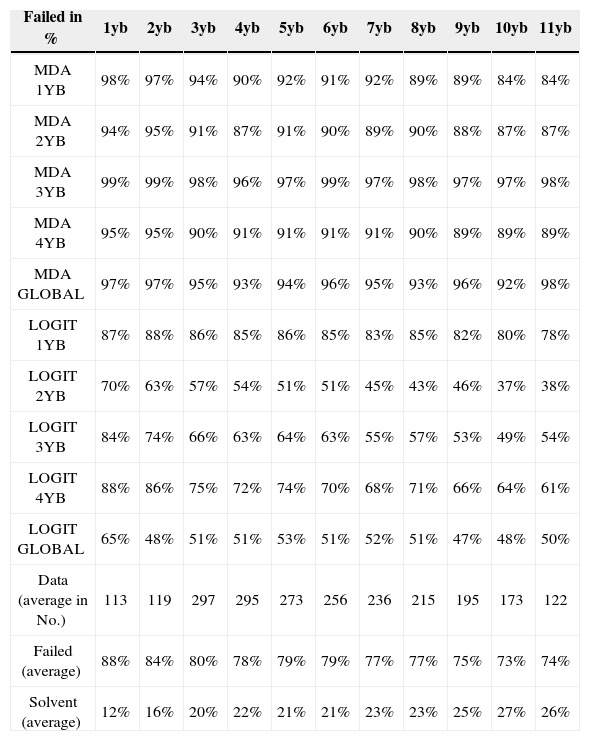
The contrast against the 2011 database, BD2b, resulted in:

Table 5.

MDA/LOGIT prediction (BD2b nov 2011)

Failed in %	1yb	2yb	3yb	4yb	5yb	6yb	7yb	8yb	9yb	10yb	11yb
MDA 1YB	98%	97%	94%	90%	92%	91%	92%	89%	89%	84%	84%
MDA 2YB	94%	95%	91%	87%	91%	90%	89%	90%	88%	87%	87%
MDA 3YB	99%	99%	98%	96%	97%	99%	97%	98%	97%	97%	98%
MDA 4YB	95%	95%	90%	91%	91%	91%	91%	90%	89%	89%	89%
MDA GLOBAL	97%	97%	95%	93%	94%	96%	95%	93%	96%	92%	98%
LOGIT 1YB	87%	88%	86%	85%	86%	85%	83%	85%	82%	80%	78%
LOGIT 2YB	70%	63%	57%	54%	51%	51%	45%	43%	46%	37%	38%
LOGIT 3YB	84%	74%	66%	63%	64%	63%	55%	57%	53%	49%	54%
LOGIT 4YB	88%	86%	75%	72%	74%	70%	68%	71%	66%	64%	61%
LOGIT GLOBAL	65%	48%	51%	51%	53%	51%	52%	51%	47%	48%	50%
Data (average in No.)	113	119	297	295	273	256	236	215	195	173	122
Failed (average)	88%	84%	80%	78%	79%	79%	77%	77%	75%	73%	74%
Solvent (average)	12%	16%	20%	22%	21%	21%	23%	23%	25%	27%	26%

Previously to the estimation of models, we have performed a factor analysis aimed at reducing the variables to a small number of synthetic and homogenous regressors. We perform the estimation for each of the time horizons, between one and four years before the failure event. In all cases we have excluded the factors whose eigenvalue was lower than one.

In the four horizons, the four variables with more weight are related to profitability and liquidity (which is measured as cashflow), indebtedness and solvency; the composition of the factors is similar with the exception of the year 4 before the failure (4yb). These results confirm the relationship between the ratios of profitability and operating cash flow (Gombola and Ketz, 1983; Pina, 1992).

Table 6.

LOGIT, MDA, MRL Contrast s/107 healthy companies (2010 BD3a)

Forecasts for healthy s/(H, F)	1yb	2yb	3yb	4yb	5yb	6yb	7yb	8yb	9yb	10yb	11yb
MDA 1 YB	39.3%	37.4%	43.9%	43.9%	44.9%	47.7%	45.8%	43.9%	46.7%	53.3%	48.1%
MDA 2 YB	43.9%	36.4%	40.2%	36.4%	41.1%	39.3%	42.1%	38.3%	38.3%	42.9%	43.3%
MDA 3 YB	9.3%	11.2%	8.4%	5.6%	8.4%	9.3%	8.4%	10.3%	7.5%	8.6%	10.6%
MDA 4 YB	42.1%	33.6%	35.5%	24.3%	29.9%	31.8%	35.5%	33.6%	33.6%	28.6%	34.6%
MDA GLOBAL	32.7%	26.2%	28.0%	23.4%	28.0%	27.1%	25.2%	24.3%	24.3%	21.9%	21.2%
LOGIT 1 YB	16.8%	20.6%	18.7%	18.7%	21.5%	27.1%	22.4%	23.4%	27.1%	28.6%	28.8%
LOGIT 2 YB	73.8%	81.3%	87.9%	91.6%	92.5%	88.8%	89.7%	90.7%	89.7%	90.5%	91.3%
LOGIT 3 YB	83.2%	81.3%	83.2%	86.9%	89.7%	89.7%	86.0%	86.0%	82.2%	85.7%	86.5%
LOGIT 4 YB	68.2%	71.0%	80.4%	80.4%	82.2%	83.2%	79.4%	76.6%	72.9%	77.1%	82.7%
LOGIT GLOBAL	75.7%	77.6%	77.6%	77.6%	82.2%	81.3%	77.6%	80.4%	76.6%	74.3%	76.9%
MRL 1 YB	3.7%	2.8%	0.0%	0.0%	0.0%	0.0%	0.0%	0.0%	0.0%	0.0%	0.0%
MRL 2 YB	14.0%	12.1%	1.9%	3.7%	2.8%	1.9%	1.9%	0.9%	1.9%	1.9%	2.9%
MRL 3 YB	0.0%	0.0%	0.0%	0.0%	0.0%	0.0%	0.0%	0.0%	0.0%	0.0%	0.0%
MRL 4 YB	20.6%	20.6%	2.8%	5.6%	3.7%	3.7%	3.7%	3.7%	5.6%	3.8%	3.8%
MRL GLOBAL	0.0%	0.0%	0.0%	0.0%	0.0%	0.0%	0.0%	0.0%	0.0%	0.0%	0.0%

The prediction capacity of the MDA and LOGIT adjustments on the healthy companies should be understood from two different perspectives. On one hand, they lack quality when it comes to rank healthy companies as non-failed in comparison to their better performance when contrasting failed companies. On the other, the contrast of the financial statements reveals that healthy companies have, or may have in the future, certain imperfections. One of the first conclusions referred to the dismissal of MRL (Linear Regression) models on the basis of their poor prediction capacity.

Contrast with DEA model

With the aim of unifying criteria, we have taken the ratios shown below on the basis of the financial-accounting information available from the 298 failed and 107 healthy companies:⁹

Outputs

TDTA=TotalDebtTotalAssets It shows the level of indebtedness with respect to the total assets. The higher this value is, the more externally dependent the company will be and, consequently, will restrict its room for manoeuvre. It explains the risk of insolvency (business failure).

CLTA=CurrentLiabilitiesTotalAssets It shows the need for immediate cover; possibility of default on its short-term liabilities. The higher its value is, the lower the liquidity will be and the higher the risk of insolvency.

Inputs

NITA=NetIncomeTotalAssets Ratio explaining the asset capacity to generate income (ROA).

CFTA=CashFlowTotalAssets It reveals how efficient the company is concerning the use of its own resources to generate liquidity (cash).

EBTA=EBITTotalAssets It reveals how efficient the company is concerning the use of its own resources to generate profit before interest and tax, i.e. it is the capacity to generate profit by the asset irrespectively of how it has been funded.

EBFE=EBITFinancialExpenses It reveals the capacity to profit before interest and tax in order to cover debt and operating costs on EBIT.

AVBAV=AddedValueBookValue It reveals the added value ratio earned by the shareholders, although we should use the market value, but SMEs are not usually quoted on the stock exchange; hence this substitution in the denominator.

CATA=CurrentAssetsTotalAssets Warehouse, Debtors, Treasury and other short-term liabilities, i.e. Current Assets. The higher the ratio is the higher the liquidity will be and, therefore, the greater the capacity to meet short-term obligations will be too.

CCTA=CirculatingCapitalTotalAssets It shows that long-term resources are funding short-term liabilities. The circulating capital is the difference between current assets and liabilities. The higher it is, the better. However, an “excessive” value would be a sign of idle resources. In addition, we could find “false negatives” as under certain financial structures the average maturity of the suppliers’ credits is higher than the average maturity of the debtors' credits, i.e. a negative circulating capital. But let's take the ratio in a strictly protective sense to cover short-term liabilities, therefore, it should always be positive (CC = FM = Ac-Pc > 0).

Without entering into the debate about the choice of the above ratios, we have made the MDA and LOGIT adjustments on our original samples, in the last five years, achieving the following results:

Table 7.

LOGIT, MDA Prediction

			LOGIT
Fail	Variables	Type	Classified correctly
Year 0	All	H	75.70%
		F	94.60%
	Excluded (O2, I6)	H	76.60%
		F	94.90%
Year -1	All	H	67.30%
		F	94.60%
	Excluded (O2, I3, I4)	H	66.40%
		F	93.90%
Year -2	All	H	64.50%
		F	92.40%
	Excluded (I4)	H	64.50%
		F	92.40%
Year -3	All	H	50.50%
		F	90.50%
	Excluded (I1, I2, I3, I4, I5)	H	51.40%
		F	91.20%
Year -4	All	H	69.20%
		F	93.90%
	Excluded (O2, I3, I4)	H	70.10%
		F	94.70%

			MDA
Fail	Variables	Type	Classified correctly
Year 0	All	H	46.70%
		F	92.20%
	Excluded (I1, I2, I5, I6, I7)	H	42.10%
		F	91.90%
Year -1	All	H	78.50%
		F	81.00%
	Excluded (I1, I3, I4, I5)	H	77.60%
		F	80.30%
Year -2	All	H	85.00%
		F	57.00%
	Excluded (I2, I3, I4)	H	84.10%
		F	81.10%
Year -3	All	H	80.40%
		F	79.40%
	Excluded (I1, I2, I3, I4, I5)	H	83.20%
		F	79.40%
Year -4	All	H	65.40%
		F	89.30%
	Excluded (O2, I1, I3, I4, I5, I6)	H	65.40%
		F	90.40%

While they are still good adjustments, the quality of the adjustment is questionable, to say the least, given the little significance of some of the ratios used in the mentioned articles.

DEA model

DEA aims to determine the hyperplanes defining a closed surface or Pareto frontier. Those units (companies, DMUs) located on the border will be efficient, as all the others will be inefficient. The DEA model¹⁰ will include the variable c_k, to allow variable returns models.

Equation 1: DEA for efficient frontier

subject to: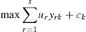

Based on the linear programming system, we have determined the set of hyperplanes defining the efficient and inefficient frontiers. We must put forward one criticism, as the determination of the efficient frontier offers scope for arbitrariness. It is based on the average value of the ratios, the best adjustment, and the best regression. In our case, we took the average values of the ratios for each year (Healthy and Failed). Therefore, this is a “relative” frontier, not absolute. Thus, we have determined both efficient and inefficient frontiers for each of the last four years. On the basis of the above approach, we have determined both the efficient and inefficient units depending on the particular case. In the case of two variables, the frontiers could be displayed as follows below:

Since we have been able to determine the set of DMUs defining the efficiency frontiers, the likelihood of financial failure or non-failure, we can add a complementary approach in order to determine whether any DMU analysed is or not efficient.

Equation 2: additive DEA

max es^− + es^+	max es^− + es^+
subject to:	subject to:
Xλ + s^− = x0	Xλ−x0 + s^− = 0
Yλ + s^+ = y0	Yλ−y0 + s^+ = 0
eλ = l	eλ = l

The above determined frontiers¹¹ provide the parameters for a hyperplane or matrix of inputs (X) and outputs (Y), which will be formed by the values of the variables (ratios) that make up the set of efficient companies and that is located on this hypothetically efficient line (hyperplane)¹²

• •

  X will be a matrix of kxn inputs and Y, a matrix of mxn outputs, with n being the number of DMUs making up the frontier, including their respective k inputs, m outputs,

• •

  e is an unit vector,

• •

  x₀, y₀: column vectors showing the inputs and outputs of the DMU subject to classification,

• •

  s^-s⁺: vectors showing the slacks of the matrix of inputs and outputs in the DMU analysed, indicating the relative efficiency; the lower the objective function is the better the position of DMU will be with respect to the frontier (efficient/inefficient),

• •

  λ will be the vector determining the intensity of development in the analysed unit with respect to the efficient (or inefficient, where appropriate) frontier.

Since we have been able to determine the efficient/inefficient hyperplane, the next step will be to determine whether an analysed unit is or not on the frontier. This will allow us to determine the stress levels in a particular unit with respect to the hypothetically efficient/inefficient ones. This is a more complex and tedious task as we will have to develop each and every analysed unit in order to place it in relation to the efficient or inefficient frontier.

This is the second step, the development of the approach shown in equation 2. Based on a given efficient/inefficient frontier formed by the matrixes Xλ, Yλ, we will analyse a particular company (DMU₀) represented by its inputs and outputs (x₀, y₀)'. The result will tell us the state of the company with respect to the efficient and inefficient frontiers, respectively.

In our case, based on the three databases discussed above, four efficient frontiers (EF) and other four inefficient (nonEF) ones were created in relation to the four years analysed. The database containing 2 966 (Healthy and Failed) companies was randomly sampled, with 402 (failed and non-failed) companies evaluated with respect to the efficient and inefficient frontiers, achieving the following results:

Table 8.

DEA-based classification

		Classified correctly	Erroneously classified	No feasible solution
On efficient frontier	Healthy	80.54%	6.01%	13.45%
	Failed	76.39%	6.29%	17.32%
On inefficient frontier	Healthy	79.80%	4.67%	15.53%
	Failed	82.67%	4.83%	12.50%

We can state that capacity to classify the analysed companies (DMUs) is significantly high. The column “Classified correctly” shows that they are not on the Pareto, or efficient, frontier but not too far from it, therefore, we do not know how inefficient they are. We cannot forget to mention that the maximum we established as a measure of comparison is itself “relative,” not an “absolute” measure, although we can define it as a “relative maximum.” The “no feasible solution” indicator shows the amount of input-output vectors to be compared with respect to the efficient frontier, which does not have a feasible solution, i.e. it provides a solution but fails with model restrictions.

Conclusions

With this study we have sought to provide evidence showing that the statistical models currently used to infer situations of financial distress and to forecast a possible financial failure might have overestimated the failure probability. Our earlier studies showed evidence supporting the ability of the MDA and LOGIT models to efficiently detect failed and insolvent companies. These models have now been applied to a contrasting random sampling exclusively made up of healthy companies in order to verify the possible existence of systematic biased opinions in the forecast. Likewise, the present study provides reasonable evidence about the reliability of the DEA model to forecast business failure. Not exempt from criticism or, if preferred, easy –immediate– applicability to the day-to-day practice of risk estimation.

In sight of the results shown above, we can confirm that DEA provides further evidence about whether a company is failing, thus, performing at a satisfactory level despite its arduous modelling. On a general basis, results show that a significant ratio of the companies that we assume are failed can correctly be “classified” as failed by the MDA, LOGIT and DEA models. But although DEA “works,” it still has significant inconveniences along with evident benefits.

Among the “benefits,” we can highlight:

• •

  DEA can be modelled for multiple inputs and outputs

• •

  DEA does not require functional links between inputs and outputs

• •

  In DEA the Decision-Making Units (DMUs) can be compared against a peer or combination of peers

• •

  In DEA, inputs and outputs can have a different measurement, for example, investment on R&D against efficiency and effectiveness of the production system in terms of redundant processes found and removed

• •

  Regarding the “inconveniences,” we should bear in mind that:

• •

  DEA cannot eliminate the extremely technical noise, even the symmetrical noise with zero mean that causes significant estimation errors

• •

  DEA is good at estimating the relative efficiency of a Decision-Making Unit (DMU) but it converges very slowly to absolute efficiency. In other words, it can tell you how well you are doing compared to your peers but not compared to a theoretical maximum.

• •

  Since DEA is a nonparametric technique, statistical hypotheses are difficult and also the main focus of a lot of research

• •

  There is a significant computing problem as a standard formulation of DEA creates a separate linear program for each DMU

We must remember that, essentially, DEA is based on a comparison exercise between peers that has been extrapolated to a “hierarchical” issue applied to financial environments with business failure risk: “healthy” / “failed.”

Perhaps the most complex issue regarding its applicability roots is the fact that the set of articles we have been discussing are not truly academic or exclusively academic. In a few cases they are even detached from a significant practical reality. Occasionally, its mathematical and cryptic levels make it difficult to implement in everyday life of financial management, who are aiming to determine the risk exposure.

In addition to the great advantages of the ratios (we can visualise immediately the correct or incorrect position of our company structure; compare our company to the relevant industry, the position of other companies at the same time as our company's life cycle) there are also limitations that need to be borne in mind:

• •

  Dispersion of the data used to obtain the reference values. The publication of reference average values is usually obtained from the average values of the sectorial information, which normally lacks additional information about the degree of dispersion of the sample data. This makes it impossible to compare our sample with the reference values.

• •

  The existing correlation between the variables forming a ratio. Something that is not implicit in the ratio concept but that subsists as an element that distorts its values and their development (i.e. its usefulness) is the potential correlation between the variables related by a ratio. This problem is aggravated with closely related ratios, invalidating its reading temporarily either for being dependant or for a high degree of correlation. In the present case:

  • •

    Clearly-related TDTA and CLTA inputs; Total Debt, Current Debt, both types of debt with respect to the Total Assets (net assets)

  • •

    NITA, CFTA, EBTA, EBFE outputs containing elements related; Net income, Cash Flow, EBIT. Sometimes dependent, as in EBTA, where the numerator BAIT and the denominator Financial Expenses are part of the EBIT.

• •

  The reference Values or standards: we have to take into account that ratios are control tools (objective against result), while any reference value should be established depending on the company, the sector of activity and the moment in the company's life cycle. The evolution of the ratio and the corrective measures against deviations should take priority in the analysis.

Furthermore, we have corroborated the existence of systematic biased opinions supporting the situations of insolvency: models perform more efficiently when their aim is to identify potentially failed companies and they commit more errors on average when they are used to evaluate solvent companies. This tendency seems to be more pronounced in the discriminant models, perhaps because they impose a discretional treatment to a particular reality –the state of insolvency– that is diffuse and liable to qualifications. In our opinion, logit models are more reliable to grasp the different realities that coexist in the generic concept of solvency. That is why they also perform relatively well between financially healthy companies.

It seems reasonable to conclude that DEA (based on LOGIT), MDA and LOGIT models should not be interpreted as mutually exclusive alternatives, but as complementary methods that, implemented in conjunction, can help fill their respective gaps.

Finally, it seems necessary to enrich the factors used as forecast variables. The ratios proved to be an excellent tool, nevertheless, the relevance of the models can improve with the help of complementary information that may corroborate –and what it seems more important to us, qualify– the forecast. In this sense, the information provided by the audit report¹³ seems to have a special informational content through indirect indicators such as the auditor turnover rate, the average duration of their contracts and the proportion of qualified reports.

We must look back at the concept of “management responsibility” in the failure process. A recent study¹⁴ states that “two out of three Spanish senior executives do not match up to the requirements of their responsibilities,” and also notes that “only 22% of middle managers think that senior executives are qualified to make sensible decisions.” When the economic situation is buoyant, it is reasonable to believe that errors, the lack of leadership, the delay in the taking of decisions are easily covered by the surplus generated by the system. But what happens when the system shrinks? The good times have hidden the low profiles of the directors. The recession or contraction periods reveal inability to make decisions. This is not a new idea but the verification of the “Peter Principle,” i.e. the verification of how important the human capital is in this process. The concept of a company as a system allows us to adopt an analytical approach to identify problems, i.e. the way all the company decisions are related to each other. Formally considered, a company is defined in Business Economics as an organisation: a complex, target-driven, socio-technical system that also has an authority structure, a system to allocate responsibilities and a control mechanism. In the last few years we have seen many examples of an irresponsible lack of control by companies and public authorities that has resulted in the recent crises. There is no need to legislate more, just exercise more control; by comparing objective to result, determining the variances that have occurred, implementing corrective actions. Simple models are the most efficient: principle of parsimony.