


The potential relationship between fund flows and performance is a remarkable topic in the mutual fund industry that has been explored by many empirical academic papers. In this work, it is shown that investors in Spanish equity funds respond to past good performance by increasing their (net) purchases, and to past poor performance by reducing their (net) purchases. However, the relationship between flows and performance appears to be non-linear. This non-linearity is different from the one observed in most of the previous research papers. These papers did not find any response to poor performance. Net purchases, purchases and redemptions are analysed separately and, as a new feature, the retail and wholesale markets of mutual funds are addressed. The comparison of the two markets reveals some interesting differences on the determinants of the financial decisions regarding purchasing or selling shares of equity funds. It was also found that investor sensitivity to poor performance is reduced in the case of more visible funds. This puzzling result, which originates in the retail segment, could be explained in terms of the market power of fund families.
The mutual fund industry is important in Spain in terms of the volume of assets under management and the number of investors who participate in the industry. At the end of 2012, according to the Spanish National Accounts, mutual funds represented 5.9% of total household wealth. According to the CNMV, in July 2013, the total assets of mutual funds under management amounted to 140,598 million euros and the number of investors totalled more than 4.7 million. Thus, one important area of research is related to the decision-making process that investors undertake when considering purchasing or selling fund shares. Hence, the aim of this paper is to shed light on the determinants of investors’ financial decisions in the mutual fund industry in Spain. Throughout the paper, two main assumptions regarding investor behaviour are going to be the drivers of the analysis. Firstly, investors learn about managerial ability from the performance of the fund. Secondly, investors face participation costs when they invest in mutual funds.
Numerous authors have investigated this issue empirically for the U.S. market. Regarding the first main assumption of this paper, the results of these studies suggest that both redemption and purchase decisions are influenced by prior performance. Earlier papers, such as Ippolito (1992), Gruber (1996), Sirri and Tufano (1998), Goetzman and Peles (1997), Chevallier and Ellison (1997) and Guercio and Tkac (2002), and more recent papers, such as Huang et al. (2007), Khorana and Servaes (2004), and Nanda et al. (2004) show a non-linear relationship between net purchases and performance of mutual funds. They found that investors made positive net purchases when a fund registered a good performance but they fail to react to poor performing funds as these funds only register low negative net purchases. These authors presented different explanations for the investors’ failure to respond to poor performing funds. They argued that investors, especially unsophisticated investors, face frictions that prevent them from withdrawing their money from poor performing funds. Among those frictions, the authors mainly highlighted advice from brokers who discourage redemptions and the investors’ aversion to realising losses.
Hence there is a well-documented asymmetric relationship between net subscriptions of mutual funds and past performance. In the literature, there are some studies describing this issue by means of theoretical models. The Berk and Green's (2004) seminal theoretical paper relates fund flows with past performance. In this paper, it is assumed that past performance is a good signal of the fund managers’ abilities. So, investors can update their belief about the fund manager's abilities through Bayes’ rule, while each time a fund's performance is known.2 This paper also makes several assumptions with respect to investors’ behaviour and fund markets that shape a frictionless environment. Thus, the authors prove that investors chase past performance. Whenever a fund has performed very well, it would receive positive net purchases and whenever a fund has performed poorly, it would show negative net purchases. In principle, the authors assert that poorly performing funds would register a large volume of redemptions and a very small volume of purchases. The opposite would arise for funds with a good performance. It is worth noting that this model fails to predict absence of reaction to medium and poorly performing funds as no participation costs are assumed.
Two subsequent papers, Huang et al. (2007) and Dumitrescu and Gil-Bazo (2013) presented extensions of the paper by Berk and Green (2004). Huang et al. (2007) incorporated frictions into the model with the intention of bringing results closer to the empirical evidence. They assume that investors enjoy different levels of information about mutual funds due to different skills to process information and the mutual fund families’ effort to make their funds visible. They also assume that investors face monitoring and transaction costs. They showed that these new assumptions make investors to purchase a lower number of funds. This would be the reason why investors only concentrate their purchases in the best performing funds. They labelled this result as ‘the winner-picking effect’. So, these authors provided a different explanation to why investors behave asymmetrically and investors’ net subscriptions register an amount much lower in medium and poorly performing funds than the positive net purchases from the best performing funds. According to these authors, the asymmetry comes from investor overreaction to purchase instead of a lack of response to poor performance.
In the same vein, Dumitrescu and Gil-Bazo (2013) assume a mutual fund market where there are two types of investors: naïve (retail investors) and sophisticated (wholesale investors). Both types of investors face different searching costs that reflect their ability to find an adequate fund and they may also be financially constrained. In addition, part of the investors is incumbent whereas others may want to participate as new entrants. These potential investors have to pay a sunk cost if they want to invest in mutual funds. Under these assumptions, the authors also find a non-linear relationship between fund flows and performance. At the same time, they prove that due to these market frictions there are funds whose performances exhibit a higher persistence.
All these papers contribute to understanding investor behaviour when they decide to participate in the mutual fund market. However, they are concentrated in only explaining mutual fund net purchases. They do not further explore the possible information that may be separately embedded in purchases and redemptions, even though the decision to purchase a mutual fund potentially differs from the decision to withdraw money from a mutual fund. In order to close this gap, literature on the determinants of purchases and redemptions in the mutual fund industry has been developed. Although this literature is still relatively scarce (Bergstresser and Poterba, 2002; O’Neal, 2004; Cashman et al., 2006; Johnson, 2007; Ivkovic and Weisbenner, 2009; Jank and Wedow, 2010), it offers interesting results on the determinants of mutual fund purchases and redemptions. Some of these papers, Bergstresser and Poterba (2002), Johnson (2007) and Ivkovic and Weisbenner (2009) also failed to find a relationship between poor performance and redemptions.3 However, the other three papers do obtain evidence that investors from the worst performing funds punish these funds by increasing redemptions. The major criticism of the former group of papers is that they examine non-random samples which may not be representative of the mutual fund universe.4
Cashman et al. (2006), one of the papers mentioned above, showed that mutual fund investors withdraw more from poorly performing funds, while they withdraw less from better performing funds. Although, there are responses to both the best and worst performing funds, the response is asymmetric. Redemptions increase more with poorly performing than they decrease in the case of the best performing funds. They also find that purchases respond to the worst and best performing funds. Previous research suggested that purchases were only sensitive to the best performing funds and not the worst performing funds. As for redemptions, purchase responses are asymmetric. The growth in purchases from the best performing funds is greater than from worst performing funds. Jank and Wedow (2010) found the same results as Cashman et al. (2006) regarding fund flows with one exception. They obtained evidence that redemptions increase with respect to performance for the best performing funds. In some of these funds, investors cash in their gains. This behaviour is known in the financial literature as the “disposition effect”.
Regarding the importance of the second main assumption of this paper – the existence of participation costs in the mutual fund market – Capon et al. (1996) pointed out that it is inadequate to consider fund performance as the only explanatory variable for mutual fund investment decisions.5 Several papers on this literature also analysed the role of participation costs in this type of market.6 In principle, three measures are used to proxy participation costs: fund fees, the market share of fund families and the number of funds offered by the fund family. Authors found that fund families with a high market share are very often the ones which make their funds’ characteristics more visible to investors. Somehow, their consumers are investors whose participation costs are lower. At the same time, these fund families are also usually the ones which charge higher fees and supply a higher number of funds to the market.
For example, Sirri and Tufano (1998) and Huang et al. (2007) showed the importance of taking participation costs into account into the analysis. They found evidence that participation costs lead to different net purchase levels. Given a level of performance, funds from the bigger families enjoy a much stronger net subscription response to performance than their rivals do. This issue was extended to purchases and redemptions by Cashman et al. (2006) and Jank and Wedow (2010). The former paper found no relationship between purchase flows and participation costs. Instead, the later paper showed that due to the higher visibility, funds from larger families exhibit higher purchases and redemptions.
Apart from past performance and participation cost, mutual fund flows are characterised by their persistence as was shown in Patel et al. (1994) and Kempf and Ruenzi (2006). These papers presented evidence that fund investors have a tendency to purchase those funds that they already purchased in the past. In the paper by Kempf and Ruenzi (2006), this investors’ behaviour is considered as non-optimal (purchasing a fund repeatedly may not be an optimal decision from among the available alternatives) and the authors coin the expression “status quo bias” to describe it. So, as other papers did, it may be important to incorporate this “status quo bias” into the analysis of the determinants of mutual fund purchases and redemptions in the Spanish market, especially in the retail segment.
Our paper is closely related to Cashman et al. (2006). In the first part of the paper, an analysis of the determinants of mutual funds purchases and redemptions for the Spanish mutual fund market is provided. This analysis is completed by studying how participation costs, measured through the market share of fund families’, affect fund flows. In the second part, due to the availability of data, and given the different characteristics of participants in these two markets, purchases and redemptions in the retail and wholesale market are analysed. In addition, an assessment on the role of participation costs in both markets is also provided. Dealing with these two markets separately is a new aspect of the literature on the determinants of mutual fund flows.
The remainder of the paper is structured as follows: Section 2 describes the dataset that is used for the study. In Section 3, a descriptive analysis of the fund purchases and redemptions flows in the Spanish market is carried out. In Section 4, an analysis of the determinants of purchases and redemptions is provided throughout an empirical model where the role is established that both their past performance and investors’ participation costs play in fund purchases and redemptions. In Section 5, by means of the same empirical model used in the previous section, and in order to study their differences, a separate analysis for the determinant of fund flows in the retail and wholesale markets is performed. Finally, Section 6 lays out the conclusions.
2DataThe empirical analysis has been performed using the reporting data the CNMV periodically receives from supervising its collective investment schemes. The database consists of annual data from the existing equity funds and fund families between 1995 and 2011, including defunct and merged funds. For the purpose of this analysis, the definition of equity funds includes pure equity funds, mixed funds and global funds. This sample of funds represents, on average, nearly 25% of total mutual fund assets. The database includes variables which either characterise the mutual fund or their fund family for each year under consideration. Based on the data, the variables to be used in the empirical analysis are the following:
- -
Net purchases: volume of purchases in the fund less redemptions over one year, divided by the size of the fund at the beginning of the year.
- -
Redemptions: volume of redemptions over one year, divided by the size of the fund at the beginning of the year.
- -
Purchases: volume of purchases in the fund, divided by the size of the fund at the beginning of the year.
- -
Measures of performance:
- ∘
Gross return: defined as the annual percentage change of the net asset value (NAV) of the fund.
- ∘
Sharpe ratio: annual gross return of the fund less the return of a risk-free asset, all divided by the standard deviation of the gross monthly returns.
- ∘
Four-FF-alpha: defined as the abnormal fund returns estimated from the Fama–French–Carhart four-factor model.7
- ∘
- -
Size: (logarithm of) total fund assets at the end of each year.
- -
Volatility: typical annualised deviation of the fund's monthly returns over the last 12 months. This is a standard risk measure to assess the profile of mutual funds.
- -
Fees: implicit periodic mutual fund fees (management fee and custody fee) are considered, as well as explicit mutual fund fees (purchase and redemption fees).
- -
Market share of the fund family: ratio between the total assets of the mutual funds managed by a fund family and the total equity fund assets in a period.
- -
Retail/wholesale fund: mutual funds are classified as wholesale if holdings per investor which are above a given minimum level amount for more than 50% of the total fund assets. Funds that do not satisfy these criteria are considered retail funds. Following Cambón and Losada (2014), who take regulatory changes into consideration during the sample period that are relevant for this purpose, the mentioned minimum holding for wholesale funds is set at €180,000 between 1995 and 1998, and at € 150,000 for the rest of the period.
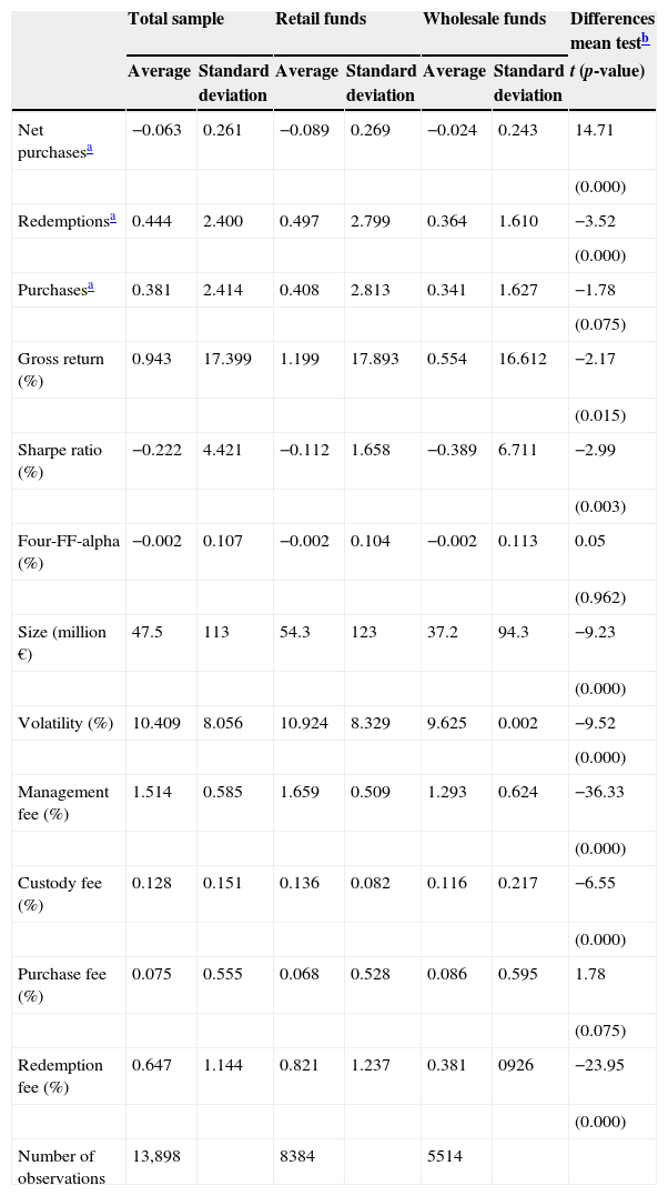
Observations with net purchases over 70% of total assets were eliminated to take into account potential errors or the existence of splits and merger funds that lead to extreme values. Table 1 shows a summary of the main descriptive statistics of the most relevant variables considered in the empirical analysis. This table considers the total sample and the retail and wholesale segments. Average net purchases in equity funds were negative between 1995 and 2010 (−6.3%). This result may be the consequence of the high volume of redemptions registered in the industry since the beginning of the crisis in 2008. The average volume of purchases8 and redemptions in retail funds was higher than the one observed in the wholesale market.
Descriptive statistics of the sample of funds.
| Total sample | Retail funds | Wholesale funds | Differences mean testb | ||||
|---|---|---|---|---|---|---|---|
| Average | Standard deviation | Average | Standard deviation | Average | Standard deviation | t (p-value) | |
| Net purchasesa | −0.063 | 0.261 | −0.089 | 0.269 | −0.024 | 0.243 | 14.71 |
| (0.000) | |||||||
| Redemptionsa | 0.444 | 2.400 | 0.497 | 2.799 | 0.364 | 1.610 | −3.52 |
| (0.000) | |||||||
| Purchasesa | 0.381 | 2.414 | 0.408 | 2.813 | 0.341 | 1.627 | −1.78 |
| (0.075) | |||||||
| Gross return (%) | 0.943 | 17.399 | 1.199 | 17.893 | 0.554 | 16.612 | −2.17 |
| (0.015) | |||||||
| Sharpe ratio (%) | −0.222 | 4.421 | −0.112 | 1.658 | −0.389 | 6.711 | −2.99 |
| (0.003) | |||||||
| Four-FF-alpha (%) | −0.002 | 0.107 | −0.002 | 0.104 | −0.002 | 0.113 | 0.05 |
| (0.962) | |||||||
| Size (million €) | 47.5 | 113 | 54.3 | 123 | 37.2 | 94.3 | −9.23 |
| (0.000) | |||||||
| Volatility (%) | 10.409 | 8.056 | 10.924 | 8.329 | 9.625 | 0.002 | −9.52 |
| (0.000) | |||||||
| Management fee (%) | 1.514 | 0.585 | 1.659 | 0.509 | 1.293 | 0.624 | −36.33 |
| (0.000) | |||||||
| Custody fee (%) | 0.128 | 0.151 | 0.136 | 0.082 | 0.116 | 0.217 | −6.55 |
| (0.000) | |||||||
| Purchase fee (%) | 0.075 | 0.555 | 0.068 | 0.528 | 0.086 | 0.595 | 1.78 |
| (0.075) | |||||||
| Redemption fee (%) | 0.647 | 1.144 | 0.821 | 1.237 | 0.381 | 0926 | −23.95 |
| (0.000) | |||||||
| Number of observations | 13,898 | 8384 | 5514 | ||||
With regard to the variables which characterise performance, the average gross return of equity funds between 1995 and 2011 was 0.94% (1.29% for retail funds and 0.55% for wholesale funds). However, the excess returns obtained from the Fama–French–Carhart model do not show a significant difference between retail and wholesale funds. Finally, it is interesting to note the differences in the fees charged for retail funds and wholesale funds. With the exception of purchase fees, it can be observed that, on average, retail funds are more expensive than wholesale funds. In particular, the average management fee, which is the most important cost of a mutual fund, is 1.66% in the retail market, while it is 1.29% in the wholesale market.
3Descriptive analysisIn this section, the flow-performance relationship for Spanish equity funds is analysed from a non-conditional framework perspective, i.e. the potential effect of other variables of interest such as the persistence of flows or the role of mutual fund fees is not taken into account. The purpose of this section is to replicate the analysis of previous academic papers (for example, Sirri and Tufano, 1998) using Spanish data. In order to evaluate the potential relationship between flows and performance, the funds are ranked according to several performance measures each year and classified in deciles. Thus, weighted averages of purchases, redemptions and net purchases are computed in order to allocate the observations in the corresponding decile.
Some of the results are presented in Fig. 1. The figure suggests that investors respond to performance, especially when it is extreme (good or bad performance). In the case of funds which record a medium performance there seems to be no relationship. In general terms, a non-linear relationship exists between flows and performance. In the case of net purchases, the type of non-linear relationship suggested in Fig. 1 is different from the one observed in most of the previous research papers9, whose authors found no empirical evidence of investor response to bad performance.10
. Note: Each year, funds are ranked into 10 groups based on the Sharpe ratio performance. The figure shows the average net purchases, purchases and redemptions for each group (divided by the size of the fund).")
The results from purchases suggest that current and potential investors respond to the good performance of funds by significantly increasing their purchases. In contrast, there is not a clear response in terms of purchases for investors of other funds. This effect, which is known in the literature as the ‘winners picking effect’, was observed in previous studies (see Sirri and Tufano, 1998; O’Neal, 2004).
The results for redemptions suggest a limited negative relationship between performance and redemptions for the group of funds with the worst performance. Fig. 1 suggests an investor punishment for poor performance by increasing their redemptions from these funds. As previously, there seems to be no relationship for funds which record a medium performance.
There is also a positive relationship for the best performing funds. The U-shaped relation for redemptions showed in Fig. 1 is not new and was also presented in prior studies. The apparent paradox whereby better performing funds experience more redemptions is explained by some authors by the need of some investors to cash in part of their gains. Some of these investors could be considered short-term traders that buy and sell fund shares rapidly.11
The relationship between net purchases and past performance also appears to be non-linear. It is observed that investors respond to good and bad performance, but they are not sensitive to funds which record a medium performance. This type of non-linearity is different from the one presented in previous academic papers. As stated earlier, they found no reaction to bad performance. Authors used different arguments for this apparent lack of response. Gruber (1996) suggested that there are two types of investors (sophisticated and disadvantaged investors) who are influenced by different factors or face some type of friction that makes their response different. Lynch and Musto (2003) pointed out that investors choose not to respond to bad performance because they expect a change in the management team after a poor result. Some other factors such as taxes or the potential aversion to realise losses (Ivkovic and Weisbenner, 2006) were also proposed as an explanation to the apparent lack of reaction to poor performance.
More recent studies (Cashman et al., 2006) suggested that the results of those earlier papers arose due to a problem with the sample period (too short). They showed that by expanding the sample, the type of non-linearity obtained is similar to the one in Fig. 1. They did obtain a response to bad performance and tried to further explore it in detail through the analysis of purchases and redemptions.
4Analysis of the determinants of investment flowsIn this section, a linear equation which relates flows and past performance of mutual funds is proposed. The three measures of performance described in Section 2 are used. Each year, funds are ranked from zero (the worst performing fund) to one (the best performing fund). Following Sirri and Tufano (1998) the ranked funds are clustered using fractile rankings in order to evaluate the potential non-linear relationship between flows and performance suggested in Fig. 1. In particular, we define three terciles as the following: the low performance tercile is defined as min (classification, 0.33), the medium performance tercile is defined as min (ranking-low performance, 0.33) and the high performance tercile is defined as ranking-low performance-medium performance. This means that if a fund is ranked by its performance at 0.90, it will have a score of 0.33 for the low performance bracket, 0.33 for the medium performance bracket and 0.24 for the high performance bracket. A fund classified by its performance at 0.50 will have a score of 0.33 for the low performance bracket, 0.17 for the medium performance bracket and 0 for the high performance bracket. Finally, a fund with a classification of 0.23 will have a score of 0.23 for the low performance bracket and 0 for the medium and high performance brackets. These terciles are used in a piecewise linear regression. This regression includes other control variables such as the size of the fund, the yield volatility and various fund fees (management and deposit, purchase and redemption fees). The equation which is estimated is as follows:
where the dependent variable is the volume of net or gross purchases or redemptions of fund i in period t divided by the assets of the fund at the end of period t−1. The explanatory variables are the fund performance in period t (for the different measures) clustered into three terciles (low performance, medium performance and high performance) and the set of variables which characterise the fund (size, volatility and fees) in the same sample period. According to the definition of the terciles, the coefficients on these piecewise decompositions of fractional ranks represent the slope of the performance-flow relationship over their range of sensitivity.12
The possibility of flow persistence, which is represented by a lag in the dependent variable, is also taken into account. Finally, the model also includes time dummies. Two types of estimates are obtained by using the Fama and MacBeth (1973) method13 and pooled OLS estimate.14 According to Petersen (2009) Fama–MacBeth coefficient estimates are more precise than pooled OLS estimates in the presence of cross sectional correlation (time effect). The results of this empirical work are statistically similar under the two approaches in most of the cases.
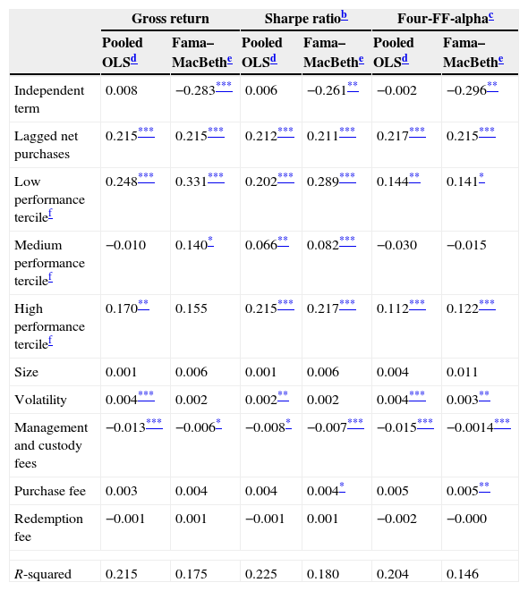
4.1Net purchasesThe determinants of annual net purchases are presented in Table 2. The results suggest a non-linear relationship between net purchases and past performance, similar to the one observed in Fig. 1. For the Fama–MacBeth and OLS estimate, the slope between net purchases and performance is clearly positive for best and worst performing funds. For funds which record a medium performance, the coefficient is only significant under the Sharpe ratio performance measure. This result is relevant because it is found that investors respond to good and bad performance. This result is in contrast with most previous academic papers which did not find a reaction to worst performing funds. In other words, investors reward best performing equity funds, increasing their (net) purchases, and punish worst performing funds by reducing their (net) purchases.
Net purchases.a
| Gross return | Sharpe ratiob | Four-FF-alphac | ||||
|---|---|---|---|---|---|---|
| Pooled OLSd | Fama–MacBethe | Pooled OLSd | Fama–MacBethe | Pooled OLSd | Fama–MacBethe | |
| Independent term | 0.008 | −0.283*** | 0.006 | −0.261** | −0.002 | −0.296** |
| Lagged net purchases | 0.215*** | 0.215*** | 0.212*** | 0.211*** | 0.217*** | 0.215*** |
| Low performance tercilef | 0.248*** | 0.331*** | 0.202*** | 0.289*** | 0.144** | 0.141* |
| Medium performance tercilef | −0.010 | 0.140* | 0.066** | 0.082*** | −0.030 | −0.015 |
| High performance tercilef | 0.170** | 0.155 | 0.215*** | 0.217*** | 0.112*** | 0.122*** |
| Size | 0.001 | 0.006 | 0.001 | 0.006 | 0.004 | 0.011 |
| Volatility | 0.004*** | 0.002 | 0.002** | 0.002 | 0.004*** | 0.003** |
| Management and custody fees | −0.013*** | −0.006* | −0.008* | −0.007*** | −0.015*** | −0.0014*** |
| Purchase fee | 0.003 | 0.004 | 0.004 | 0.004* | 0.005 | 0.005** |
| Redemption fee | −0.001 | 0.001 | −0.001 | 0.001 | −0.002 | −0.000 |
| R-squared | 0.215 | 0.175 | 0.225 | 0.180 | 0.204 | 0.146 |
Purchases in the fund less redemptions over a year, divided by the size of the fund at the beginning of the year.
Annual Sharpe ratio is calculated by subtracting the risk-free rate from the gross return of the fund and dividing the result by the standard deviation of the fund return.
Another point of interest is related to the potential asymmetry of this non-linear relationship. The coefficient for worst performing funds across different specifications is generally higher than the coefficient for high performing funds, although the regular hypothesis tests do not reject the equality of these coefficients.15
This result can be compared with results in Cashman et al. (2006). They concluded that the response to good performance appears to be stronger than that for bad performance. As long as they detected a symmetric response in redemptions, they stated that the asymmetry for net purchases should be originated by inflows sensitivity.
Apart from the relationship between flows and performance, which is the main goal of this work, it is very interesting to test the impact of other variables included in the model on fund flows. The presence of persistence in the net purchases of mutual funds is shown robustly. The coefficient associated with this persistence indicates that over 21–22% of net purchases of equity funds tend to be repeated over the next year. The persistence of flows has also been shown in other research papers.16
The relationship between net purchases and fees is negative and only significant for management and custody fees. Ceteris paribus, more expensive equity funds (i.e. funds with higher management and custody fees) experience less net purchases. This result is also shown in Cashman et al. (2006) and it may be a sign that for investors, the expected performance of expensive funds is not higher than the performance of cheaper funds. The costs associated with entry and exit from a fund are not significant when net purchases are considered, but several differences will be observed when fund purchases are analysed.
Regarding the effect of other relevant characteristics of the fund, the results are mixed. There seems to be a positive relationship between the volatility of the fund and net purchases, but the coefficient related to the size of the fund is not significant.
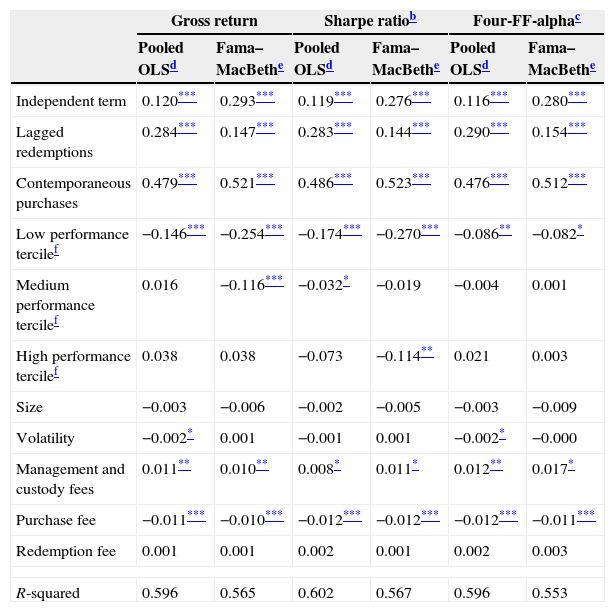
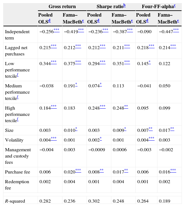
4.2RedemptionsRegarding the search for evidence in the case of redemptions and purchases, two alternative models have been considered: the first model takes into account the potential persistence of flows and the second model also incorporates the potential effect of short-term trading. In order to control for this possible rapid trading, contemporaneous flows are introduced in the regressions. The relationship between flows and performance presents some differences under these different specifications. We are going to provide some comments on the estimations of both models but only the table with the results for the model with persistence and short term trading will be presented. This second specification is preferred as long as it could be more representative of the industry given the evidence found in a number of studies.17
The results for redemptions when controlling only for persistence are consistent with a U-shaped form for the redemption–performance relationship. Under this specification, investors punish worst performing funds by increasing redemptions, a fact that was not found in the previous studies. However, they do not reward best performing funds by reducing redemptions. On the other hand, they increase redemptions from high performing funds. This U-shaped curve for redemptions was also shown in Jank and Wedow (2010). Under this specification the coefficients related to flow persistence are positive and significant, with levels that range from 27% to 47% depending on the method of estimation.
When rapid trading is introduced into the model, the U-shaped form for redemptions does not hold (see Table 3). Investors continue to punish worst performing funds by increasing redemptions. However, the relationship between redemptions and high performing funds becomes very weak. Moreover, when the coefficient is significant, it states a negative flow-performance relationship; better funds are rewarded by reducing their withdrawals.
Redemptiona (with persistence and short-term trading).
| Gross return | Sharpe ratiob | Four-FF-alphac | ||||
|---|---|---|---|---|---|---|
| Pooled OLSd | Fama–MacBethe | Pooled OLSd | Fama–MacBethe | Pooled OLSd | Fama–MacBethe | |
| Independent term | 0.120*** | 0.293*** | 0.119*** | 0.276*** | 0.116*** | 0.280*** |
| Lagged redemptions | 0.284*** | 0.147*** | 0.283*** | 0.144*** | 0.290*** | 0.154*** |
| Contemporaneous purchases | 0.479*** | 0.521*** | 0.486*** | 0.523*** | 0.476*** | 0.512*** |
| Low performance tercilef | −0.146*** | −0.254*** | −0.174*** | −0.270*** | −0.086** | −0.082* |
| Medium performance tercilef | 0.016 | −0.116*** | −0.032* | −0.019 | −0.004 | 0.001 |
| High performance tercilef | 0.038 | 0.038 | −0.073 | −0.114** | 0.021 | 0.003 |
| Size | −0.003 | −0.006 | −0.002 | −0.005 | −0.003 | −0.009 |
| Volatility | −0.002* | 0.001 | −0.001 | 0.001 | −0.002* | −0.000 |
| Management and custody fees | 0.011** | 0.010** | 0.008* | 0.011* | 0.012** | 0.017* |
| Purchase fee | −0.011*** | −0.010*** | −0.012*** | −0.012*** | −0.012*** | −0.011*** |
| Redemption fee | 0.001 | 0.001 | 0.002 | 0.001 | 0.002 | 0.003 |
| R-squared | 0.596 | 0.565 | 0.602 | 0.567 | 0.596 | 0.553 |
Annual Sharpe ratio is calculated by subtracting the risk-free rate from the gross return of the fund and dividing the result by the standard deviation of the fund return.
Under this model specification, the persistence of redemptions remains significant, although less intense. The coefficient for contemporaneous purchases (short-term trading) is significant and ranges between 48% and 52%. The relationship between redemptions and purchase fees is negative while the coefficient for management fees becomes significant and positive. Under this latter result, more costly managed funds experience more redemptions. This result suggests that higher management and custody fees are not interpreted at least by some investors as a signal of a future higher performance, prompting increased redemptions from these funds.
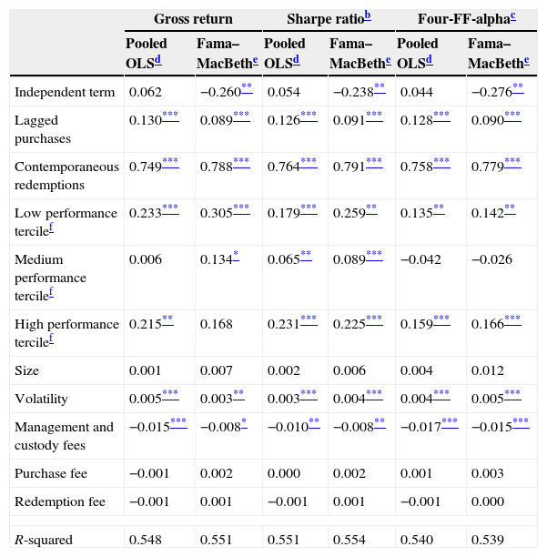
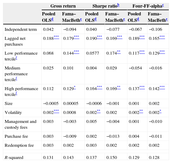
4.3PurchasesIn order to analyse the determinants of purchases to equity funds, a similar procedure was followed as for redemptions. When rapid trading is not taken into account, the results suggest a strong relationship between high performing funds and purchases for all specifications and performance measures. Under this pattern of behaviour, commonly known as ‘winner-picking effect’, investors intensively purchase the best performing funds. There seems to be no relationship between purchases of funds and performance for funds which record a medium and poor performance.
The coefficient for purchase persistence is highly significant and ranges from 25% to 35%. The results also show a positive relationship between volatility and purchases. According to this result, investors are willing to invest their money in higher volatility funds, which are likely to be seen as funds with higher expected yields. It is important to notice that this behaviour is compatible with the presence of short-term investors in the market.
After controlling for short-term trading (see Table 4), a positive relationship between gross purchase flows and high performing funds is also observed. Furthermore, a positive relationship between purchases and low performing funds is identified. This later result suggests that investors respond to good performance, by increasing purchases, and to bad performance, by reducing purchases. The sensitivity to low and high performance is found to be similar, so the non-linear relationship could be symmetric. It is important to remember that in the case of redemptions, only a significant response to bad performance was detected. This result concludes an asymmetric relationship exists between redemptions and performance.
Purchasesa (with persistence and short-term trading).
| Gross return | Sharpe ratiob | Four-FF-alphac | ||||
|---|---|---|---|---|---|---|
| Pooled OLSd | Fama–MacBethe | Pooled OLSd | Fama–MacBethe | Pooled OLSd | Fama–MacBethe | |
| Independent term | 0.062 | −0.260** | 0.054 | −0.238** | 0.044 | −0.276** |
| Lagged purchases | 0.130*** | 0.089*** | 0.126*** | 0.091*** | 0.128*** | 0.090*** |
| Contemporaneous redemptions | 0.749*** | 0.788*** | 0.764*** | 0.791*** | 0.758*** | 0.779*** |
| Low performance tercilef | 0.233*** | 0.305*** | 0.179*** | 0.259** | 0.135** | 0.142** |
| Medium performance tercilef | 0.006 | 0.134* | 0.065** | 0.089*** | −0.042 | −0.026 |
| High performance tercilef | 0.215** | 0.168 | 0.231*** | 0.225*** | 0.159*** | 0.166*** |
| Size | 0.001 | 0.007 | 0.002 | 0.006 | 0.004 | 0.012 |
| Volatility | 0.005*** | 0.003** | 0.003*** | 0.004*** | 0.004*** | 0.005*** |
| Management and custody fees | −0.015*** | −0.008* | −0.010** | −0.008** | −0.017*** | −0.015*** |
| Purchase fee | −0.001 | 0.002 | 0.000 | 0.002 | 0.001 | 0.003 |
| Redemption fee | −0.001 | 0.001 | −0.001 | 0.001 | −0.001 | 0.000 |
| R-squared | 0.548 | 0.551 | 0.551 | 0.554 | 0.540 | 0.539 |
Annual Sharpe ratio is calculated by subtracting the risk-free rate from the gross return of the fund and dividing the result by the standard deviation of the fund return.
Purchase persistence is still relevant when considering rapid trading, although the coefficient is much lower. The relationship between purchases and volatility is also positive. Under this specification, the relevant fees for investors are those related to management and custody. Higher management costs could be associated with lower ex-post yields instead of being a sign of good managerial skills, as investors reduce purchases to those funds.
4.4The effect of market powerSome researchers have highlighted the effect of investor participation costs on the relationship between fund flows and performance (see, for example, Huang et al., 2007). They argue that investors face two types of costs when investing in the mutual fund industry. The first one is related to the information cost of collecting and evaluating the characteristics of the funds before investing. The other type of cost is related with the transaction costs of purchasing or redeeming funds. In the current analysis, these costs are directly incorporated into the models estimated in the previous section. These authors test whether the possibility of reducing search costs should lead to an increase in the sensitivity of fund flows to past performance or not. As long as the information costs for individual investors are not noticeable, these studies usually take as proxies some fund or fund family characteristics that are related to the visibility of the fund: marketing expenses, the size of the fund family measured by the assets under management or the variety of funds offered.
Under this hypothesis, mutual funds with lower participation costs should show greater flow sensitivity to performance in comparison with funds which have higher participation costs, especially in the medium performance segment. In these papers, mutual funds with lower participation costs are associated with more visible funds. The conclusions of research into the subject are mixed. Some papers do not find any change in the sensitivity of net purchases whereas others do find some variation in the response of flows for medium and high performing funds.
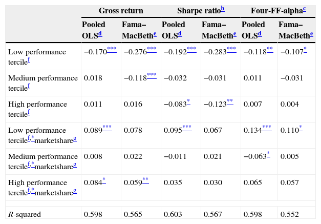
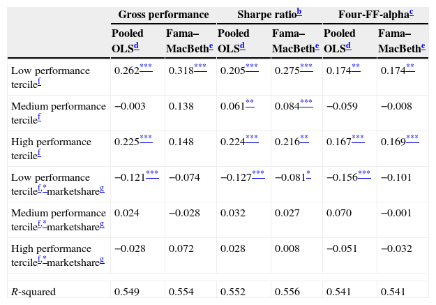
In this study, visibility is introduced by means of several proxies such as the fees, the market share of fund families18 and the variety of categories or funds offered by the fund family.19 Only the results when using “market share” as a proxy for visibility are reported. The results are rather similar under all specifications. Table 5 provides results for redemptions and Table 6 for purchases. As seen in both tables, the effect of visibility appears to only be significant for the group of worst performing funds under the Pooled-OLS estimation method. This result is in contrast with previous theories which found a change of sensitivity in the segment of medium performing funds. Moreover, the change in investor sensitivity to performance for more visible funds does not correspond to what is expected from the theory. Investors should invest strongly in more visible funds due to the decrease in transaction costs.
The effect of visibility on redemptionsa (with persistence and short-term trading).
| Gross return | Sharpe ratiob | Four-FF-alphac | ||||
|---|---|---|---|---|---|---|
| Pooled OLSd | Fama–MacBethe | Pooled OLSd | Fama–MacBethe | Pooled OLSd | Fama–MacBethe | |
| Low performance tercilef | −0.170*** | −0.276*** | −0.192*** | −0.283*** | −0.118** | −0.107* |
| Medium performance tercilef | 0.018 | −0.118*** | −0.032 | −0.031 | 0.011 | −0.031 |
| High performance tercilef | 0.011 | 0.016 | −0.083* | −0.123** | 0.007 | 0.004 |
| Low performance tercilef,*marketshareg | 0.089*** | 0.078 | 0.095*** | 0.067 | 0.134*** | 0.110* |
| Medium performance tercilef,*marketshareg | 0.008 | 0.022 | −0.011 | 0.021 | −0.063* | 0.005 |
| High performance tercilef,*marketshareg | 0.084* | 0.059** | 0.035 | 0.030 | 0.065 | 0.057 |
| R-squared | 0.598 | 0.565 | 0.603 | 0.567 | 0.598 | 0.552 |
Redemptions over one year divided by the size of the fund at the beginning of the year. The original regressions include other control variables that are not presented in the table for simplicity reasons.
Annual Sharpe ratio is calculated by subtracting the risk-free rate from the gross return of the fund and dividing the result by the standard deviation of the fund return.
Low performance tercile is defined as Min (classification 0.33), medium performance tercile is defined as Min (0.33, classification – low) and high performance tercile is defined as Rank-Medium-Low.
The effect of visibility on purchasesa (with persistence and short-term trading).
| Gross performance | Sharpe ratiob | Four-FF-alphac | ||||
|---|---|---|---|---|---|---|
| Pooled OLSd | Fama–MacBethe | Pooled OLSd | Fama–MacBethe | Pooled OLSd | Fama–MacBethe | |
| Low performance tercilef | 0.262*** | 0.318*** | 0.205*** | 0.275*** | 0.174** | 0.174** |
| Medium performance tercilef | −0.003 | 0.138 | 0.061** | 0.084*** | −0.059 | −0.008 |
| High performance tercilef | 0.225*** | 0.148 | 0.224*** | 0.216** | 0.167*** | 0.169*** |
| Low performance tercilef,*marketshareg | −0.121*** | −0.074 | −0.127*** | −0.081* | −0.156*** | −0.101 |
| Medium performance tercilef,*marketshareg | 0.024 | −0.028 | 0.032 | 0.027 | 0.070 | −0.001 |
| High performance tercilef,*marketshareg | −0.028 | 0.072 | 0.028 | 0.008 | −0.051 | −0.032 |
| R-squared | 0.549 | 0.554 | 0.552 | 0.556 | 0.541 | 0.541 |
Purchases over one year, divided by the size of the fund at the beginning of the year. The original regressions include other control variables that are not presented in the table for simplicity reasons.
Annual Sharpe ratio is calculated by subtracting the risk-free rate from the gross return of the fund and dividing the result by the standard deviation of the fund return.
Low performance tercile is defined as Min (classification 0.33), medium performance tercile is defined as Min (0.33, classification – low) and high performance tercile is defined as Rank-Medium-Low.
According to the evidence found in the group of worst performing funds, redemptions from high visible funds (that is, belonging to high market share fund families) are less intensive than redemptions from the rest of the funds. Similarly, inflows to high visible funds are less intensive than inflows to other funds. In other words, the investors’ punishment for bad performance, by increasing redemptions or decreasing purchases, is lower for more visible funds. Although this issue deserves a more detailed analysis, this counterintuitive result could be explained in terms of the potential presence of market power in the industry. According to Cambón and Losada (2014), evidence for the Spanish mutual fund industry suggests the existence of a certain degree of market power which is mainly exhibited by large fund families. These companies enjoy a higher market share in the industry by increasing the number of funds and/or categories of funds offered to investors. These large fund families could sell a substantial part of their worst performing funds to less sophisticated investors who, in general, are less sensitive to past performance and to other relevant fund characteristics.
5Retail versus wholesale investors5.1Net purchases – retail and wholesale marketsGiven the results shown so far, it is appropriate to split the sample in order to distinguish between retail and wholesale investors. As the characteristics of both types of investors are different, they may behave differently and contribute to the aggregate in a different manner.
As Tables 7 and 8 show, the analysis reveals a notable persistence in the behaviour of net purchases in both markets, although it is higher in the retail market, where 21–22% of the net purchases registered in a year are repeated during the following year. This percentage is between 16% and 18% in the wholesale market. This higher persistence in the retail market could be evidence of a higher relevance of the status quo bias in this market.20 This means that retail investors may make investment decisions which are suboptimal more frequently than wholesale investors.
Net purchasesa – retail market.
| Gross return | Sharpe ratiob | Four-FF-alphac | ||||
|---|---|---|---|---|---|---|
| Pooled OLSd | Fama–MacBethe | Pooled OLSd | Fama–MacBethe | Pooled OLSd | Fama–MacBethe | |
| Independent term | −0.256*** | −0.419*** | −0.236*** | −0.387*** | −0.090 | −0.447*** |
| Lagged net purchases | 0.215*** | 0.212*** | 0.212*** | 0.211*** | 0.218*** | 0.214*** |
| Low performance tercilef | 0.344*** | 0.375*** | 0.294*** | 0.351*** | 0.145* | 0.122 |
| Medium performance tercilef | −0.038 | 0.191* | 0.074* | 0.113 | −0.041 | 0.050 |
| High performance tercilef | 0.184*** | 0.183 | 0.248*** | 0.248** | 0.095 | 0.099 |
| Size | 0.003 | 0.010* | 0.003 | 0.009* | 0.007** | 0.017** |
| Volatility | 0.004*** | 0.001 | 0.002* | 0.001 | 0.004*** | 0.003 |
| Management and custody fees | −0.004 | 0.003 | −0.0009 | 0.0006 | −0.003 | −0.002 |
| Purchase fee | 0.006 | 0.020*** | 0.008** | 0.017** | 0.006 | 0.016*** |
| Redemption fee | 0.002 | 0.004 | 0.001 | 0.004 | 0.001 | 0.002 |
| R-squared | 0.282 | 0.236 | 0.302 | 0.248 | 0.264 | 0.189 |
Purchases in the fund less redemptions over a year, divided by total fund assets at the beginning of the year.
Annual Sharpe ratio is calculated by subtracting the risk-free rate from the gross return of the fund and dividing the result by the standard deviation of the fund return.
Net purchasesa – wholesale market.
| Gross return | Sharpe ratiob | Four-FF-alphac | ||||
|---|---|---|---|---|---|---|
| Pooled OLSd | Fama–MacBethe | Pooled OLSd | Fama–MacBethe | Pooled OLSd | Fama–MacBethe | |
| Independent term | 0.042 | −0.094 | 0.040 | −0.077 | −0.067 | −0.106 |
| Lagged net purchases | 0.188*** | 0.179*** | 0.190*** | 0.169*** | 0.189*** | 0.165*** |
| Low performance tercilef | 0.068 | 0.144*** | 0.0577 | 0.174** | 0.117*** | 0.129*** |
| Medium performance tercilef | 0.025 | 0.101 | 0.004 | 0.029 | −0.054 | −0.016 |
| High performance tercilef | 0.112 | 0.129* | 0.164*** | 0.169** | 0.137*** | 0.142*** |
| Size | −0.0005 | 0.00005 | −0.0006 | −0.001 | 0.001 | 0.002 |
| Volatility | 0.002*** | 0.0008 | 0.002** | 0.002 | 0.002** | 0.002* |
| Management and custody fees | 0.003 | −0.003 | 0.005 | −0.004 | 0.001 | −0.010 |
| Purchase fee | 0.003 | −0.009 | 0.002 | −0.013 | 0.004 | −0.011 |
| Redemption fee | 0.003 | 0.002 | 0.003 | 0.002 | 0.002 | 0.002 |
| R-squared | 0.131 | 0.143 | 0.137 | 0.150 | 0.129 | 0.128 |
Purchases in the fund less redemptions over a year, divided by total assets of the fund at the beginning of the year.
Annual Sharpe ratio is calculated by subtracting the risk-free rate from the gross return of the fund and dividing the result by the standard deviation of the fund return.
Regarding sensitivity to performance in the retail market, when gross return and the Sharpe ratio are considered as a measure of performance, investors exhibit a strong positive sensitivity to worst performing funds.21 As is expected, in the medium bracket, investors showed no reaction to performance. As it was previously discussed, this lack of sensitivity may be a sign of high participation costs for these investors when they decide to invest in equity funds. As for the worst performing funds, investors also exhibit a positive sensitivity to the best performing funds. These results are in line with the evidence provided by Cashman et al. (2006) and Jank and Wedow (2010).
However, sensitivity to worst performing funds is found to be higher than to best performing funds. This result is new in studies of this type. Previous papers (for example the ones cited above) found evidence of the opposite. Later, it will be shown that this result could have arisen because the level of purchases for worst performing funds in the retail market is no different from in the wholesale market, while the level of redemptions is notably higher.
One important feature of the results for the retail market is the lack of sensitivity with respect to performance when this is measured by means of the factor model. One possible explanation to this issue may be that this measure of performance is not used by retail investors when they consider investment decisions regarding mutual funds.
It should be also pointed out that among the control variables only the purchase fee is significant. Since the estimated coefficient is positive, this variable could be seen by retail investors as a sign of a higher expected performance for the fund.
In the case of the wholesale market, sensitivity with respect to performance is observed when this is measured by means of either the Sharpe ratio or the factor model. This type of investor shows sensitivity to the best and worst performing funds. However, these sensitivities are clearly lower than the ones found in the retail market. Another difference between the two markets is that in the wholesale market there are no clear differences on how investors react to the worst and best performance, since both coefficients are rather similar.
On the other hand, wholesale investors do not show any sensitivity to medium performing mutual fund. Similar to retail investors, this lack of sensitivity may be a reflection that wholesale investors also face participation costs when investing in these investment schemes. With respect to the other variables, only mutual fund volatility is significant when the estimate is by pooling OLS.22 The relationship between this variable and net purchases is found to be positive. This means that wholesale investors prefer to invest in funds with risk.
One important difference between the results obtained in this paper and other related papers is that, in this case, only purchase fees are significant for retail investor while no fee is significant for wholesale investors. Previous papers, for example Cashman et al. (2006) and O’Neal (2004), found that fees were significant variables to explain the behaviour of investors in mutual funds.
5.2Redemptions – retail and wholesale marketsIn order to analyse redemptions in the retail and wholesale markets, two estimations for each market have been performed. The first estimation assumes the existence of flow persistence. This means that redemptions are considered a function of past redemptions, as argued by Cashman et al. (2006), performance and group of control variables. In the second estimation, short-term trading of mutual funds is incorporated as a key variable to explain redemptions. There are authors, (Chalmers et al., 2001; Greene and Hodges, 2002; Zitzewitz, 2006) who argue there is a large volume of short-term trading in the mutual fund market.23
Comments on the results of both models are provided but only tables for the preferred model of each market (retail and wholesale) are presented. In this respect, it is difficult to know the real behaviour of retail investors regarding short-term trading. Although for a given volume of redemptions, part of them could be due to short-term trading that amount could be far from being one of the main drivers of retail investors’ behaviour. In Ispierto and Villanueva (2009), it is shown that this type of investor is not sophisticated. Thus, it is difficult to assume that these investors’ skills and knowledge allow them to make investments by means of complex strategies.24 For these reasons, and according to the characteristics of retail investors’, one could think that not considering short-term trading could be a closer approach to retail investors’ behaviour, whereas considering short-term trading could be a better approach to wholesale investors’ behaviour. In an endeavour to be consistent with previous analyses, only the gross return and Sharpe ratio are considered as measures of performance in the retail market, and only Sharpe ratio and factor model performance measures are considered in the analysis of the wholesale market.
Hence, in the retail market, when short-term trading is not considered, redemptions and performance measured by gross returns show a U-shaped relationship (see Table 9). Investors penalise more those funds with worst performance and investors of the best funds try to withdraw their money from the best performing funds with greater intensity as the fund performs better. This means investors in the best performing funds would find it profitable to cash in part of the gains. However, the robustness of this last result should be taken with care. When the Sharpe ratio is considered as the measure of performance, investors are not so keen to cash in the gains from the best performing funds.
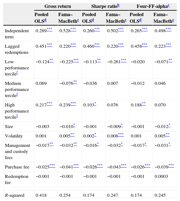
Redemptionsa – retail market (with persistence).
| Gross return | Sharpe ratiob | Four-FF-alphac | ||||
|---|---|---|---|---|---|---|
| Pooled OLSd | Fama–MacBethe | Pooled OLSd | Fama–MacBethe | Pooled OLSd | Fama–MacBethe | |
| Independent term | 0.289*** | 0.528*** | 0.260*** | 0.502*** | 0.265*** | 0.498*** |
| Lagged redemptions | 0.451*** | 0.220*** | 0.460*** | 0.220*** | 0.458*** | 0.223*** |
| Low performance tercilef | −0.124** | −0.225*** | −0.113** | −0.261*** | −0.020 | −0.071** |
| Medium performance tercilef | 0.069 | −0.076** | −0.036 | 0.007 | −0.012 | 0.046 |
| High performance tercilef | 0.217*** | 0.239*** | 0.103* | 0.076 | 0.188** | 0.070 |
| Size | −0.003 | −0.010* | −0.001 | −0.009* | −0.001 | −0.012* |
| Volatility | 0.001 | 0.005** | 0.002* | 0.008*** | 0.001 | 0.005** |
| Management and custody fees | −0.017** | −0.032** | −0.016* | −0.032* | −0.017* | −0.031* |
| Purchase fee | −0.025*** | −0.041*** | −0.026*** | −0.043*** | −0.026*** | −0.039*** |
| Redemption fee | −0.001 | −0.001 | −0.001 | −0.001 | −0.001 | 0.0003 |
| R-squared | 0.418 | 0.254 | 0.174 | 0.247 | 0.174 | 0.245 |
Annual Sharpe ratio is calculated by subtracting the risk-free rate from the gross return of the fund and dividing the result by the standard deviation of the fund return.
The two other important results from this table are: firstly, there is strong evidence that the independent term of the regression is significant and positive. There is a large volume of redemptions annually which cannot be explained either by the fund's characteristics or by investor persistence in redemptions. Secondly, decisions on redemptions by retail investors’ appear to be influenced by fund fees. Mutual funds in the retail market with higher management, depositary and purchase fees would register less redemptions. These two results could show evidence that fund families in the retail market and, especially those which charge higher fees, could influence their clients by exercising their market power against them. When fund families belong to financial conglomerates, the first result could be interpreted as the ability of fund families’ to switch money from equity funds to other investments which are more profitable for their conglomerates. The second result could reflect the ability of reducing redemptions from retail investors who may think of moving to another fund that does not belong to his current fund family.
When short-term trading is introduced the results change slightly. Basically, the U-shape with respect to performance does not hold when this is measured by means of gross return. In addition, the expected result of funds with the worst performance suffering more withdrawals also takes place when redemptions are controlled for short-term trading. Another interesting feature from this estimation is that the variable size is negative and significant. This result could also explain why fund families, especially those which manage large funds, could enjoy market power because, as is shown, these fund family investors withdraw less money from their funds regardless of the fund's performance. It is important to notice that the largest funds are usually managed by the largest fund families owned by credit institutions.25
In the wholesale market, when short-term trading is not considered, there is no strong evidence that redemptions are sensitive to fund performance. The most important variable to explain redemptions in this market is the amount of redemptions in the previous year. This means that there is a high persistence, specifically, between 33.1% and 43.3%, of previous year redemptions are repeated in the following year. Only the variable purchase fee appears marginally as significant when the estimate procedure is OLS.
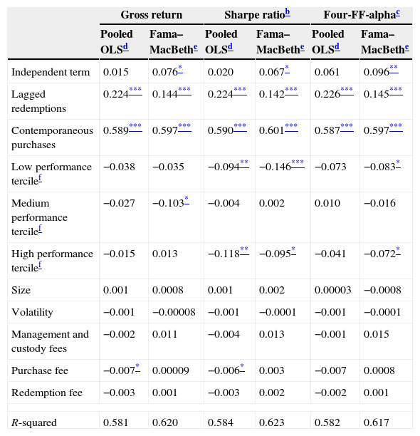
When short-term trading is introduced in the analysis of redemptions, that is our preferred model for the wholesale investors taking into account the characteristics of the participants of this market, it can be observed that a negative and significant relationship exists between redemptions and performance for the worst and the best performing funds (see Table 10).
Redemptionsa – wholesale market (with persistence and short-term trading).
| Gross return | Sharpe ratiob | Four-FF-alphac | ||||
|---|---|---|---|---|---|---|
| Pooled OLSd | Fama–MacBethe | Pooled OLSd | Fama–MacBethe | Pooled OLSd | Fama–MacBethe | |
| Independent term | 0.015 | 0.076* | 0.020 | 0.067* | 0.061 | 0.096** |
| Lagged redemptions | 0.224*** | 0.144*** | 0.224*** | 0.142*** | 0.226*** | 0.145*** |
| Contemporaneous purchases | 0.589*** | 0.597*** | 0.590*** | 0.601*** | 0.587*** | 0.597*** |
| Low performance tercilef | −0.038 | −0.035 | −0.094** | −0.146*** | −0.073 | −0.083* |
| Medium performance tercilef | −0.027 | −0.103* | −0.004 | 0.002 | 0.010 | −0.016 |
| High performance tercilef | −0.015 | 0.013 | −0.118** | −0.095* | −0.041 | −0.072* |
| Size | 0.001 | 0.0008 | 0.001 | 0.002 | 0.00003 | −0.0008 |
| Volatility | −0.001 | −0.00008 | −0.001 | −0.0001 | −0.001 | −0.0001 |
| Management and custody fees | −0.002 | 0.011 | −0.004 | 0.013 | −0.001 | 0.015 |
| Purchase fee | −0.007* | 0.00009 | −0.006* | 0.003 | −0.007 | 0.0008 |
| Redemption fee | −0.003 | 0.001 | −0.003 | 0.002 | −0.002 | 0.001 |
| R-squared | 0.581 | 0.620 | 0.584 | 0.623 | 0.582 | 0.617 |
Annual Sharpe ratio is calculated by subtracting the risk-free rate from the gross return of the fund and dividing the result by the standard deviation of the fund return.
Other relevant result under this specification is that past redemptions and contemporaneous purchases are key variables to explaining investor behaviour regarding redemptions. Depending on the estimate procedure, the persistence in redemption ranges between 14% and 22% whereas 59% to 60% of the redemptions over a year can be explained by the purchases made during that year. This last figure might indicate that short-term trading is important in this submarket.
The analysis shows that past redemptions play a key role in both markets to explain the current level of this variable. There is also another similarity between both markets. There is a negative and significant relationship between the performance and redemptions for the worst performing funds, even though this relationship appears to be stronger in the retail market.
There are also differences between these markets. Investors in the best performing funds behave in a totally different way depending on the market. Retail investors prefer to withdraw part of their money while wholesale investors prefer to maintain their money in those funds. A possible explanation for this difference is that retail investors face more financial constraints and prefer to cash in earnings. Another result that highlights the difference between the two types of investor is that volatility is significant and positive for retail investors, but not for wholesale investors. This suggests that the former are more risk averse than the later. Finally, another important difference is that the market power of fund families’ is stronger in the retail market than in the wholesale market, as suggested by the results obtained from the independent terms, the fund size and the fees.
5.3Purchases – retail and wholesale marketsAs for redemptions, two estimations for each market have been performed although only one table with the results of the preferred specification for each market is presented. Under the first model specification, fund purchases are a function of the fund's performance and persistence in addition to other control variables, such as fees or fund size. Under the second model specification, contemporaneous redemptions are added as an explanatory variable to study how short-term mutual fund trading affects the behaviour of investors regarding their purchasing decisions.
Again, it is difficult to establish the real behaviour of retail investors for short-term trading. Although, part of the purchases could be due to short-term trading, those purchases could be far from being one of the main drivers of retail investors’ behaviour. The perceived differences in the level of financial sophistication between retail and wholesale investors suggest that in the retail market the model that does not take into consideration short term trading could be a better approach where as in the wholesale market the model with short term trading would be preferred. Additionally, only the gross return and Sharpe ratio are considered as relevant measures of performance in the retail market and only the Sharpe ratio and factor model performance measures are considered in the wholesale market.
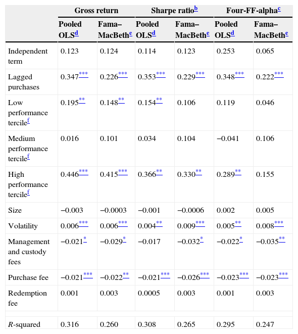
As is shown in Table 11, the model estimated without taking into consideration short-term trading suggests a strong relationship between purchases and performance in the retail market. Purchases have a positive and significant relationship with the best and the worst performing funds. This relationship is found to be stronger for the best performing funds. In the case of funds which record a medium performance, such a relationship is not found. The other important variable to explain the purchases made by retail investors is the persistency of the purchases. Past year purchases explained between 22.6% and 35.3% of the current year's purchases.
Purchasesa – retail market (with persistence).
| Gross return | Sharpe ratiob | Four-FF-alphac | ||||
|---|---|---|---|---|---|---|
| Pooled OLSd | Fama–MacBethe | Pooled OLSd | Fama–MacBethe | Pooled OLSd | Fama–MacBethe | |
| Independent term | 0.123 | 0.124 | 0.114 | 0.123 | 0.253 | 0.065 |
| Lagged purchases | 0.347*** | 0.226*** | 0.353*** | 0.229*** | 0.348*** | 0.222*** |
| Low performance tercilef | 0.195** | 0.148** | 0.154** | 0.106 | 0.119 | 0.046 |
| Medium performance tercilef | 0.016 | 0.101 | 0.034 | 0.104 | −0.041 | 0.106 |
| High performance tercilef | 0.446*** | 0.415*** | 0.366** | 0.330** | 0.289** | 0.155 |
| Size | −0.003 | −0.0003 | −0.001 | −0.0006 | 0.002 | 0.005 |
| Volatility | 0.006*** | 0.006*** | 0.004** | 0.009*** | 0.005** | 0.008*** |
| Management and custody fees | −0.021* | −0.029* | −0.017 | −0.032* | −0.022* | −0.035** |
| Purchase fee | −0.021*** | −0.022** | −0.021*** | −0.026*** | −0.023*** | −0.023*** |
| Redemption fee | 0.001 | 0.003 | 0.0005 | 0.003 | 0.001 | 0.003 |
| R-squared | 0.316 | 0.260 | 0.308 | 0.265 | 0.295 | 0.247 |
Annual Sharpe ratio is calculated by subtracting the risk-free rate from the gross return of the fund and dividing the result by the standard deviation of the fund return.
It is also important to note two other results. Firstly, retail investors who invest in equity funds prefer funds with higher volatility. If one considers the standard profile of retail investors in Spain, this result is counterintuitive since retail investors are usually risk averse. This result may arise either because investor decisions are driven by mutual funds advisors who make retail investors to invest in highly risky funds or because there is a self-selection regarding the profile of these funds’ investors. Only retail investors with an appetite for risk invest in this type of fund. Secondly, funds with higher purchasing fees have lower purchases. In this case, retail investors may find purchase fees as a barrier to investing in mutual funds.
When short-term trading is considered in the retail market the results are not very different. It is also seen that there is a strong relationship between the worst and the best performing funds and the purchases registered in a year. However, in this case, the slope is higher for worst performing funds than for the best performing ones, in contrast with what happens in the absence of contemporary redemptions. Remarkable persistence in purchases is also registered after the introduction of short-term trading and again purchases are higher for riskier funds.
Meanwhile, in the wholesale market, the estimates without contemporary redemptions suggest that there is a positive relationship between the best performing funds and purchases. However, this relationship is much weaker for worst performing funds and funds which record a medium performance. A strong persistence in purchases can also be observed in this model. Between 29.5% and 34.1% of the current year's purchases are repeated in the following year. In this market, volatility also matters as riskier funds register higher purchases. This could indicate that few wholesale investors are risk averse.
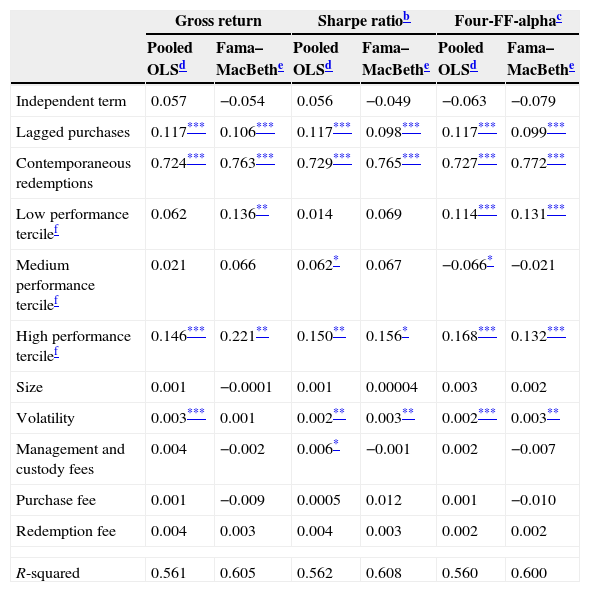
When short-term trading is incorporated in the factor model for the wholesale market, a strong, positive relationship between performance and purchases is found for both the worst and the best performing funds (see Table 12). When performance is measured by the Sharpe ratio, this relationship is not found to be so strong. In this case, only the relationship is significant and positive for the best performing funds.
Purchasesa – wholesale market (with persistence and short-term trading).
| Gross return | Sharpe ratiob | Four-FF-alphac | ||||
|---|---|---|---|---|---|---|
| Pooled OLSd | Fama–MacBethe | Pooled OLSd | Fama–MacBethe | Pooled OLSd | Fama–MacBethe | |
| Independent term | 0.057 | −0.054 | 0.056 | −0.049 | −0.063 | −0.079 |
| Lagged purchases | 0.117*** | 0.106*** | 0.117*** | 0.098*** | 0.117*** | 0.099*** |
| Contemporaneous redemptions | 0.724*** | 0.763*** | 0.729*** | 0.765*** | 0.727*** | 0.772*** |
| Low performance tercilef | 0.062 | 0.136** | 0.014 | 0.069 | 0.114*** | 0.131*** |
| Medium performance tercilef | 0.021 | 0.066 | 0.062* | 0.067 | −0.066* | −0.021 |
| High performance tercilef | 0.146*** | 0.221** | 0.150** | 0.156* | 0.168*** | 0.132*** |
| Size | 0.001 | −0.0001 | 0.001 | 0.00004 | 0.003 | 0.002 |
| Volatility | 0.003*** | 0.001 | 0.002** | 0.003** | 0.002*** | 0.003** |
| Management and custody fees | 0.004 | −0.002 | 0.006* | −0.001 | 0.002 | −0.007 |
| Purchase fee | 0.001 | −0.009 | 0.0005 | 0.012 | 0.001 | −0.010 |
| Redemption fee | 0.004 | 0.003 | 0.004 | 0.003 | 0.002 | 0.002 |
| R-squared | 0.561 | 0.605 | 0.562 | 0.608 | 0.560 | 0.600 |
Annual Sharpe ratio is calculated by subtracting the risk-free rate from the gross return of the fund and dividing the result by the standard deviation of the fund return.
There is also evidence of persistence in wholesale investors’ purchases when contemporary redemptions are considered. Between 9.8% and 11.7% of the current year's purchases are explained by the previous year's purchases. The other variable that is found to be significant is volatility. Funds with high volatility receive more purchases. Hence, there is strong evidence that wholesale investors who decide to participate in this market are not risk averse.
When the two markets are compared, two important differences arise. The sensitivity with respect to performance is much stronger in the retail market. Moreover, the responses to the best and worst performances are asymmetric in the case of the retail market while in the wholesale market it appears to be symmetric. It is also found that retail investors’ reactions to best performing funds are greater than for worst performing funds. This result is in line with the findings of Sirri and Tufano (1998) who found similar result for U.S. equity funds. These authors argue that fund visibility can explain these results. More visible good performing funds can be easily observed by most investors, who purchase these funds strongly.
6ConclusionsThe potential relationship between flows and performance in the mutual fund industry has been analysed in many academic papers. Most of these papers suggested some type of asymmetry in that relationship. In this study, the sensibility of investment flows (net and gross) to performance in the Spanish equity fund segment between 1995 and 2011 was assessed. Evidence was found of a non-linear relationship between net purchases and performance. This result is different from the non-linear relationship observed in previous research papers which did not detect any response to bad performance. Participation costs, investor heterogeneity, the aversion to realising loses or fiscal reasons were often argued to explain this apparent lack of sensitivity of investors to poor performance. In the Spanish market, investors reward funds that perform well by increasing their (net) purchases. They also punish poorly performing funds by reducing their (net) purchases, and they do not show any response to medium performance. The type of non-linear relationship found seems to be (statistically) symmetric.
The analysis for gross investment flows took into account the existence of flow persistence and the presence of short-term traders in the market, both of which have been documented in recent papers. The results for redemptions suggest that investors punish bad performance by increasing their withdrawals; on the other hand, they do not react to medium and good performance. As regards purchases, the empirical evidence identifies a similar investor response to both good and bad performance. So, an asymmetric relationship between redemptions and performance and a symmetric relationship between purchases and performance were found.
The potential influence of participation costs in the mutual funds industry was also considered. It is usually assumed that funds which exhibit lower informational costs should show a higher sensitivity in their flow performance relationship. However, the results from more visible funds suggest that investor punishment for bad performance is lower. Despite visibility, retail investors face higher participation costs. This counterintuitive result could be explained in terms of market power. According to Cambón and Losada (2014), the evidence for the Spanish mutual fund industry suggests the existence of a certain degree of market power which is mainly enjoyed by large fund families. These large fund families could place a substantial part of their worst performing funds to less sophisticated investors who, in general, are less sensitive to past performance and to other relevant fund characteristics.
The analysis of the flow performance relationship for both retail and wholesale segments revealed some common patterns and some differences. Both types of finding can be explained by the characteristics of the investors in each segment and the presence of a certain degree of market power in the industry. Firstly, high and (statistically) significant flow persistence for both types of investor was detected, slightly stronger for retail investors. Secondly, it was found that both retail and wholesale investors respond to performance, although retail investor's sensitivity was higher.
As regards redemptions, there is evidence that both types of investor punish poor performance by increasing their withdrawals. However, they show a very different response to good performance. Wholesale investors reward better performing funds by reducing redemptions, whereas retail investors increase redemptions from better performing funds. Retail investors possibly find it profitable to cash in part of their gains. For purchases, the most important difference is observed in the sensitivity to good performance: retail investors purchase good funds more intensely. This retail investor pattern, which is coined the ‘winner-picking effect’, can be explained in terms of the participation costs they face. As long as it is very costly for them to obtain proper information when trying to invest in a fund, they strongly increase the purchases of those better performing funds that are more visible. On the other hand, it is possible that not only past performance but other relevant fund or manager characteristics also are considered in the decision to purchasing funds by wholesale investors.
In conclusion, it was found that investors in Spanish equity funds are sensitive to past good and poor performance. This result differs from most previous papers that had studied the US market. In particular, it was seen that investors punish badly performing funds by reducing (net) flows, and reward better performing funds by increasing (net) flows. The analysis of purchases, which points to some differences in terms of the symmetry of this sensitivity, turns out to be very interesting when the effect of fund visibility is incorporated. The results suggest that the sensitivity of investors to poor performance is reduced for more visible funds. They could be explained in terms of market power as those counterintuitive results take places in the retail segment, according to preliminary results. It is possible that large fund families, most of them belonging to credit institutions, place a substantial part of their badly performing funds with less sophisticated investors that, in general, are less sensitive to past performance and to other relevant characteristics of the funds. The existence of different types of investors has also been used in other relevant papers to explain some empirical findings in the mutual fund industry (see for example Dumitrescu and Gil-Bazo, 2013).
We acknowledge the data provided from our colleagues by the Statistics department at CNMV and the comments by an anonymous referee, Elias Lopez and the participants at the XXI Foro de Finanzas. The usual disclaimer applies.
They are the members of the Research, Statistics and Publications Department, CNMV.
Bayes’ rule links the degree of belief in a proposition (in this case, the manager's ability to pick assets which perform well for the funds under his management) before and after accounting for evidence (in this case, past performance).
Jank and Wedow (2010) is the only paper mentioned in this paragraph which studies a dataset composed of mutual funds from outside the US market. These authors examine a database composed of mutual funds from the German market.
Bergstresser and Poterba (2002) study the 200 largest mutual funds. Johnson (2007) studies fewer funds, all from a single no-load fund family. Ivkovic and Weisbenner (2009) only examine the trading behaviour of retail investors within a single discount brokerage.
The importance of this assumption also appears in the 1990 Consumer Report survey of mutual fund investors published by the Bureau of Labor Statistics of the United States. Although performance was rated as the most important overall factor, several additional factors could be also relevant: amount of sales charge, management fees or type of fund family. These factors could be considered as proxies for participation costs in the mutual fund industry.
Sirri and Tufano (1998), Huang et al. (2007), Cashman et al. (2006), Guercio and Tkac (2002), Khorana and Servaes (2004), Nanda et al. (2004), Goetzman and Peles (1997) and Elton et al. (2004).
The Fama–French–Carhart model is an extension of the traditional asset pricing model (CAPM) which uses only one variable to describe the return on shares (the excess of the market return on the risk free rate). The Fama–French–Carhart model adds three additional factors: (i) differences of returns between a portfolio of small versus large caps, (ii) differences of returns from a portfolio of high versus low book-to-market ratio companies and (iii) a proxy for momentum.
Statistically we do not find a significant difference between the average volume of purchases in the retail and the wholesale market (see Table 1).
Sirri and Tufano (1998), Ippolito (1992), Goetzman and Peles (1997), Chevallier and Ellison (1997), Guercio and Tkac (2002) or Berk and Green (2004).
In Section 1, these authors’ arguments regarding mutual fund investors’ lack of response to bad performance are set out in detail.
Evidence of “rapid trading” has been shown, for example, in Bhargava and Dubosky (2001), Chalmers et al. (2001) and Goetzman et al. (2001).
Although funds ranked over 0.66 will have a score for the low performance bracket (of 0.33) and for the medium performance bracket (of 0.33), the slope of the performance-flow relationship in the low and medium performance terciles will not be determined by the scorings of these funds. The variability we need to estimate the slope is introduced by the scorings of the low performing funds (ranked under 0.33). The same applies to mid performing funds with respect to the slope in the low performance tercile.
Under the Fama–MacBeth approach, the coefficient estimates are obtained as the average of the cross-sectional regression estimates. This methodology provides standard errors corrected for cross-sectional correlation. This is a very desirable property in the presence of time effects, as is the case in this paper. In addition, we computed robust-standard errors to correct for time series autocorrelation (individual effects).
Given the existence of residual correlation across time, an OLS estimate was calculated, clustering standard errors by time. However, it is important to note that the correlation may not be totally corrected by this methodology.
According to the 95% confidence intervals, we cannot reject the equality of both coefficients.
See Bhargava and Dubosky (2001), Chalmers et al. (2001), Goetzman et al. (2001), Greene and Hodges (2002) and Zitzewitz (2006).
Fund affiliation with a large family effect (brand recognition) is shown in Capon et al. (1996) and Goetzman and Peles (1997). Sirri and Turfano (1998) also find that large families will receive greater inflows and that the flow-performance relationship will be stronger for larger complexes.
Elton et al. (2004) find that funds that are part of a family offering a variety of other types of fund attract significantly more cash flows.
Status quo bias is a cognitive bias characterised by the preference for a current state of affairs. The current baseline (or status quo) is taken as a reference point, and any change from that baseline is perceived as a loss. Status quo bias has been attributed to a combination of loss aversion and the endowment effect. An individual weighs the potential losses of switching from the status quo more than the potential gains. Status quo bias should be distinguished from a rational preference for the status quo, as when the current state of affairs is objectively superior to the available alternatives, or when imperfect information is a significant problem. A large body of evidence shows that a status quo bias frequently affects human decision-making. See, for example, Samuelson and Zeckhauser (1988).
Sirri and Tufano (1992) find that gross returns, which are not adjusted for risk, appear to drive fund growth. They suggest that “naïve retail trend chasers” are even more responsive to the “noisier” measure of unadjusted performance.
Remember that OLS estimate is clustered by year.
These authors use daily flow data from TrimLabs to demonstrate the ability of rapid traders to systematically transfer wealth from long-term investors to themselves. Rapid traders move quickly in and out (or, for that matter, out and in) of stale mutual fund prices (NAV). Alternatively, and perhaps more benignly, it could be the case that there is a relevant percentage of mutual fund investors that, for whatever reason, move in and out in a short period of time.
In O’Neal (2004), the author argues short-trading is a very complex investment strategy. It is difficult to take as a credible assumption that the average retail investor could afford such a strategy either financially or because of its complexity.

