Innovative knowledge-based system for forecasting daily hotel operations amid external events using multi-source data: A time-varying parameter state-space model

Abstract

Forecasting hotel occupancy during external shocks is particularly challenging due to their disruptive effects. This study develops a forecasting framework that integrates multisource data using a time-varying parameter state-space model (TVP-SSM). In this framework, search engine data (SED) are used to construct exogenous variables, intervention variables are used to reflect the severity of external shocks, and holiday and weekend dummy variables are used to capture the seasonal effect. The empirical study used a dataset from the hospitality industry in Hangzhou, China, covering the period from October 1, 2019, to October 28, 2021, and identified the COVID-19 pandemic as an external shock. The results show that TVP-SSM can effectively simulate the dynamic impact of external events and the periodical effect on hotel occupancy. Additionally, the prediction accuracy of TVP-SSM with intervention variables and periodical variables (TVP-SSM-1) exceeds that of competitive models. Specifically, compared to the naïve model and TVP-SSM without intervention variables and periodic variables (TVP-SSM-2), the prediction accuracy, measured by the root mean square error (RMSE) and mean absolute percentage error (MAPE), increased by 86 % and 87 %, respectively, and by 74 % and 76 %, respectively. These results indicate that the forecasting framework proposed in this study exhibits superior forecasting performance and demonstrates its capability for dynamic impact analysis of hotel occupancy at the industry level under external shocks.

Introduction

In the hospitality industry, enhancing the accuracy of occupancy forecasting can improve resource allocation and support the development of effective contingency plans (Wu et al., 2017; Zhang et al., 2021b; Gao et al., 2024; Waris & Mohd Suki, 2025). Previous studies have made many attempts to forecast tourism demand accurately. Song and Li (2008) classified tourism demand forecasting methods into three groups: time series models (Assaf et al., 2019; Dong et al., 2023), cross-section and panel econometric models (Hu & Song, 2019; Wen et al., 2019; Nicholas, 2021), and artificial intelligence technologies (He et al., 2021; Bi et al., 2022; Zhao et al., 2022). However, when tourism is affected by exceptional external shocks, such as natural disasters, terrorist attacks, or public health crises, the stability of these models is undermined (Zhang & Lu, 2022).

In response to external shocks, scholars have sought to enhance the accuracy of tourism forecasting models. Among them, the optimization of the model is the most direct path. Intervention analysis (Ozdogan & Ozdogan, 2023) and dynamic regression (Prilistya et al., 2021) are introduced into the tourism demand forecasting model. Additionally, expanding the diversity of data sources is also considered an effective means. Some literature integrates search engine data (SED; Liu et al., 2019; Hu et al., 2021b; Chen et al., 2024), web traffic data (Yang et al., 2013; Gunter & Önder, 2016; Emili et al., 2020; Li et al., 2023; Zhang et al., 2019), social media data (Pezenka & Weismayer, 2020; Xue et al., 2023; Zhan et al., 2024; Zhu et al., 2024; Sun et al., 2025; Tan et al., 2025), and other types of tourist flow data to discuss the construction of tourism demand forecasting models.

However, most previous studies assumed constant model parameters and could only reflect the overall impact of external events on tourism demand. However, in reality, the impact of external intervention would gradually change in real-time, according to policy and other factors. Therefore, this study draws on the concept of time-varying parameter (TVP) models to construct a TVP state-space model (TVP-SSM)-based forecasting framework utilizing multisource heterogeneous data, which aims to capture the dynamic impact of external shocks on hotel occupancy. The TVP models were transferred into the state-space model (SSM) in this framework. The dynamics of the impact of external events can be characterized by the different forms of state equations in the SSM.

To address this issue, this study proposes a new forecasting framework that leverages multiple sources of data. First, the COVID-19 pandemic is regarded as an external shock, and holiday variables are treated as periodic variables. Then, multisource data such as SED and official statistics are integrated to perform this study. Second, by constructing the TVP-SSM, the impact of the COVID-19 pandemic at different stages is incorporated into the state equations, capturing the dynamic effects of external events on tourism demand forecasting. Further, empirical analyses are conducted based on the daily data of Hangzhou and Zhoushan (China). Then comparative analyses and sensitivity analyses are performed to verify the performance of the proposed TVP-SSM model.

The remainder of the study is organized as follows. Section 2 presents the literature review. Section 3 introduces the methodology, while Section 4 describes the dataset and variables. Sections 5 and 6 provide the empirical analysis and robustness checks, respectively. Finally, Section 7 summarizes the conclusions and outlines directions for future research.

Literature review

Tourism demand forecasting with SED

Internet data, especially SED, have become increasingly popular for forecasting tourism demand (Li et al., 2020; Sun et al., 2022). Customers are prone to using online search engines, such as Baidu and Google, to plan their trips. The volume of search keywords serves as an early indicator of tourist activity, making it possible to use SED to anticipate fluctuations in tourism demand (Dergiades et al., 2018; Sun et al., 2019). Xiang and Pan (2011) analyzed the interplay between tourists’ online queries and demand for a particular destination. They confirmed a direct relationship between growth in search queries and tourism demand.

Moreover, previous literature has shown that SED can significantly contribute to gains in prediction accuracy (Li & Law, 2019; Zhang et al., 2020; Wickramasinghe & Ratnasiri, 2021). For instance, Pan et al. (2012) directly introduced five search keywords into models to analyze the demand for hotel rooms. They found that including Google search data in the model could significantly enhance prediction accuracy. Similarly, Xie et al. (2021) and Zhang and Tian (2022) incorporated the Baidu Index into a least squares support vector regression model and gated recurrent unit network, respectively, showing that Baidu search data could effectively boost the prediction accuracy of tourism inflow. Zhang et al. (2023a) proposed a gated recurrent unit network-based deep learning framework that can learn the disturbance of events and the regular pattern of tourist arrival volume. To compare SED across different search engines, Yang et al. (2015) used data from Google and Baidu to model tourism inflows. They found that Google search data were more suitable for forecasting international tourism demand, whereas Baidu search data were more suitable for forecasting tourism demand within China.

Tourism demand forecasting under interventions

Tourism demand is easily influenced by exceptional external shocks, such as pandemics and terrorist attacks, resulting in poor prediction accuracy for time series models. Based on time series models, Box and Tiao (1975) pioneered an intervention analysis model to reflect the influence of exceptional external events, and this method is widely used to forecast tourism demand (Chen et al., 2007; Jiao & Chen, 2019). For example, Lai and Lu (2005) applied intervention analysis models to examine the impact of 9/11 on airline passenger flow in the United States. They found that passenger flow declined sharply within one to two months after 9/11, but the effect was sudden and temporary. Fan et al. (2023) explored how COVID-19 changed Chinese residents’ travel behaviors and factors that influenced Chinese residents’ actual travel and willingness to travel. Seong and Lee (2021) extended intervention analysis beyond the autoregressive integrated moving average (ARIMA) models to exponential smoothing models. They found that exponential smoothing models can more easily incorporate complex seasonality into the analysis. However, intervention analysis models are limited by the pattern and number of exceptional external events.

To address the limitations related to both the pattern and the frequency of exceptional external events, researchers have sought to incorporate their impact directly into models using dummy variables. Prilistya et al. (2021) used ARIMAX and seasonal dynamic regression models to analyze the influence of the COVID-19 pandemic on foreign tourists to Indonesia. Wu et al. (2022) proposed the mixed data sampling models (MIDAS) to monitor and forecast the hotel occupancy rates under the impact of the pandemic. Additionally, Yang et al. (2022) evaluated the usefulness of online search queries in boosting forecasting accuracy during the COVID-19 pandemic. They found that the usefulness of search queries in forecasting is associated with pandemic severity. However, these models, which assume constant parameters, can only reflect the average impact of the pandemic on tourist arrivals.

Tourism demand forecasting with the state-space model

Parameter estimation of TVP models can be realized by transforming the model form into a SSM (Athanasopoulos et al., 2011; Song et al., 2011). SSM can adjust variable coefficients in real time using the Kalman filter, which exhibits strong robustness (Kalman, 1960). For that reason, SSM has been applied to gross domestic product forecasting (Aruoba et al., 2016), stock forecasting (Monache, Petrella & Venditti, 2020), international trade (Srdelić & Dávila-Fernández, 2024), and currency price fluctuation forecasting (Shafiqah et al., 2022).

In the tourism field, Song and Wong (2003) constructed a TVP model by SSM to analyze the dynamic relationship between tourist income and tourism demand. Similarly, Wu et al. (2012) constructed an almost ideal demand system model with TVPs based on an SSM. They verified the dynamic relationship between the prices for tourism-related goods and services and their demand. Xiong et al. (2018) used SSMs to forecast China’s inbound tourist arrivals from six countries. They found that income level exerts the most significant influence on tourist arrivals, and that SSMs outperform both linear regression and ARIMA models over longer time horizons.

An SSM can also effectively capture the dynamic impacts of exceptional external events on tourism demand. For instance, Jorge-Gonzalez et al. (2020) constructed a structural time series model with TVPs using an SSM to reflect the impact of five different exceptional external events on tourism flow.

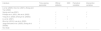
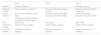
Concluding remarks from the literature review

Table 1 summarizes the forms of models and the types of data included in previous studies. From Table 1, one can note that there has been progress in the sense of the variables and models applied. However, there are still open questions regarding tourism demand forecasting under external shocks. Therefore, specific literature gaps require extension of the existing methods.

Table 1.

Structure of models in previous literature on tourism demand forecasting.

Literature	Time-varying parameter	Official statistics	SED	Periodical variables	Intervention variables
Li et al. (2020); Xie et al. (2021); Zhang and Tian (2022)			√
Seong and Lee (2021)		√			√
Prilistya et al. (2021); Wu et al. (2022)		√			√
Yang et al. (2022); Zhang et al. (2023a)		√	√		√
Liu et al. (2021)	√	√	√
Wu et al. (2012); Lee et al. (2020)	√	√
Jorge-Gonzalez et al. (2020); Zhang et al. (2022b)	√	√			√
Our study	√	√	√	√	√

First, the application of SED extends the scope of information that describes changes in tourism demand, improving the timeliness and accuracy of forecasting. However, although the search trends correlate with the occurrence of external shocks, SED cannot fully describe the effects of external events on tourism demand. Yang et al. (2022) have verified that SED was of little use in improving the accuracy of forecasting when the COVID-19 pandemic was severe. This study aims to use SED, together with variables capturing the impact of external events, to provide a more comprehensive description of the business environment.

Second, to accurately reflect the impact of external events on tourism demand, models such as the intervention analysis model, the ARIMAX model, and the MIDAS model have been proposed with relatively good prediction accuracy. However, the intervention analysis models are only used in conjunction with univariate models such as ARIMA and can only reflect the impact of a single external shock. The coefficients in ARIMAX and MIDAS models are fixed, which makes it impossible to simulate a flexible trend. This paper constructs TVP models using SSMs to capture the varying influence of extreme events. TVP-SSM can reflect the dynamics in the influence of external shocks according to changes in the variable parameters.

Third, existing studies have demonstrated that SSMs can better capture the dynamic dependence relationship between variables, making them suitable for reflecting the influence of exceptional external shocks on tourism demand. However, few studies have simultaneously utilized SSMs, SED, official statistics, intervention variables, and periodic variables to forecast tourism demand when external shocks influence tourism demand. In this study, a TVP-SSM is constructed to reflect the correlation between hotel occupancy, SED, and official statistics and the dynamic impact of intervention and periodical variables on hotel occupancy.

Research objectives

In recent years, research on tourism demand forecasting has made significant progress, and related studies have verified the effectiveness of SED (Zhang, 2023b; Wu et al., 2024), holiday variables (Hu et al., 2021a), etc., on tourism demand forecasting. However, most of the existing studies use univariate models for tourism forecasting (Apergis et al., 2016; Semenoglou et al., 2023), which negatively affects the accuracy of the forecasting model when external events impact it. The objective of this paper is to develop a tourism demand forecasting framework with strong dynamic forecasting capabilities under external event shocks by integrating multiple data sources. The main contributions of this study are as follows.

First, the prediction model integrates multisource data. In this study, different variables are integrated into the model in the form of explanatory variables or dummy variables, including external intervening variables, tourist flows, SED, holiday variables, weekend variables, etc., which reflect the impact of different factors on hotel occupancy comprehensively, and provide a firm support to improve the predictive ability of the model.

Second, a TVP model was constructed in state space form. Existing studies only capture the average impact of external events on forecasting results, without accounting for the dynamic evolution of these impacts. However, in real life, the impact of external events is multistage, and the impacts at each stage are dynamically changing (Sun et al., 2023). In this situation, governmental prevention and control as an intervention is also time-varying. The proposed TVP-SSM model can effectively reflect the dynamic impact of external events on hotel occupancy, further improving the accuracy of the forecasting model.

Third, the constructed prediction framework is scalable and generalized. The multisource data used in this study include official statistics, SED, intervention variables, and periodic variables. A time-varying parametric state-space model-based dynamic forecasting framework is constructed, which can effectively quantify the impact of various external events on tourism demand. The framework can be extended to other fields such as macroeconomic forecasting, traffic flow forecasting, etc. Based on this framework, other multisource data can be further considered and applied to other fields, such as macroeconomic forecasting, traffic flow forecasting, etc.

Methodology

State-space model

SSMs are generally applied to multivariate time series analysis. The multisource data used in this study include official statistics, SED, intervention variables, and periodic variables. SSMs estimate parameters according to the Kalman filter algorithm, which has accuracy and robustness (Kalman, 1960). Compared with time series models, such as ARIMA and Autoregressive Conditional Heteroskedasticity model, SSMs can reflect the dynamic dependence relationship between variables, and often have higher prediction accuracy (Shafiqah et al., 2022). The form of SSM is given as

where Eqs. (1) and (2) are the measurement equation and state equation, respectively; yt and αt are an observable vector and an unobservable state vector, respectively; zt is a measurement matrix, and dt is a matrix of exogenous variables; ut and εt are unrelated disturbance terms that are normally and independently distributed (mean is 0, and variances are Ht and Qt respectively); Trepresents the number of periods covered.

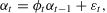
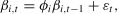
From the expression in Eq. (2), it can be observed that the change follows a first-order autoregressive process. The TVP model can be transformed into SSMs based on Eqs. (1)–(3). The form of the TVP model is given as

where β0 is the intercept; βi,t and γj denote time-varying and fixed coefficients to be estimated, respectively; xi,t and zj,t denote the exogenous variables with time-varying and fixed coefficients, respectively; m and n are the number of exogenous variables with time-varying and fixed coefficients, respectively. If the elements of the matrix ϕi in Eq. (5) are equal to unity, the state equation reduces to a random walk process (Song & Wong, 2003):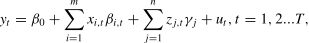

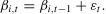
If the state equation can be expressed as a random walk, the parameter vector βi,t is considered nonstationary.

LASSO regression model

To handle big data, the LASSO regression can be used for dimensionality reduction (Uniejewski et al., 2019; Tian et al., 2021). The LASSO model contracts the regression coefficients by constructing a penalty function (Tibshirani, 1996). When the coefficient of a variable decreases to zero, that variable is excluded from the model. Based on the regression function yt=β0+∑j=1Nβjxj,t, the estimator of the LASSO regression model is given as

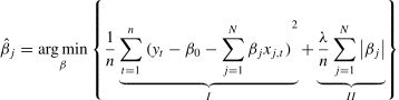
On the right-hand side of Eq. (7), terms Ⅰ and Ⅱ represent the residual sum of squares and penalty term, respectively; λ denotes the penalty level, N stands for the number of variables and n is the sample size. The value of λ is critical in LASSO regression. According to Schwarz (1978), the Bayesian information criterion is used to determine the appropriate value of λ.

Data transformation

Multiple variables have different orders of magnitude and dimensions. Directly incorporating these variables into models will affect the accuracy (Zhang & Lu, 2022). Therefore, normalization should be performed prior to analysis. This study employs linear min–max normalization to enhance training efficiency. The final retained keywords are indexed by j=1,2...Nand periods by t=1,2...T. Then, xjt* is the number of queries with the j-th keyword during period t. The normalization is carried out as follows:

where minjxjt* and maxjxjt* denote operators returning the smallest and largest values of xjt*, respectively. The combined keyword variable (xt) is then obtained as

Evaluation metrics

When evaluating the predictive accuracy of forecasting models, the root mean square error (RMSE) and mean absolute percentage error (MAPE) are the two most commonly used measures. The calculation of the two measures proceeds as follows:

where yt and y⌢t represent the actual value and predicted value during the forecast period, respectively; T is the length of the forecast period.

To avoid prediction contingency arising from data sampling, the Diebold and Mariano (DM) test is employed to assess whether there is a significant difference between the two forecasting models. The DM test relies on the loss differential (Dt) to compare prediction ability of the two models (Zhang et al., 2021a):

where L(ei,t) is a loss function (this study uses RMSE and MAPE) and ei,t represents the residual at time t calculated based on model i.

Based on Eq. (12), the DM statistic is obtained as follows:

where D¯t and σDt represent the mean and standard deviation of Dt, respectively. The standard deviation is calculated following Diebold and Mariano (2002), and the resulting sampling distribution follows a standard normal distribution. If DM<0, then Model 1 outperforms Model 2 in terms of prediction ability.

Forecasting framework

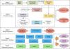
This study proposes an integrated approach (Fig. 1) that incorporates SED and intervention variables into hotel occupancy forecasts.

Fig. 1.

Forecasting framework for hotel occupancy.

This framework includes the following five steps:

• Step 1: Selection of search keywords. The basic keywords are determined based on the four elements of tourism (food, accommodation, transportation, and attractions). Then, automatic recommendation technology (Baidu Index) is used to obtain extended keywords.

• Step 2: Constructing the variables. First, the search keywords in Step 1 are selected by considering the Pearson correlation coefficient and LASSO regression (where hotel occupancy is used as a covariate or the dependent variable) and then aggregated to obtain SED variables. Second, the stationarity and cointegration tests are performed on the SED variables. Finally, the intervention and periodic variables are specified in the form of an impulse function.

• Step 3: Estimation of models. After constructing the TVP-SSM with the variables specified in Step 2, the Maximum Likelihood estimation and Kalman filter are applied to estimate its parameters. The significance is also tested.

• Step 4: Comparison of forecasting performance. Based on RMSE, MAPE, and DM statistics, the prediction results of TVP-SSM with intervention and periodical variables (TVP-SSM-1) are compared with those of benchmark models to verify the superiority of TVP-SSM-1.

• Step 5: Robustness analysis. Based on the Hangzhou and Zhoushan data sets, three cases are designed to further validate the robustness of the TVP-SSM model: Case 1 changes the ratio of the training set and testing set, Case 2 replaces the response variables, and Case 3 changes the data set.

Data and variables

This study is based on multisource data, including official statistics, SED, intervention variables, and periodic variables. Official statistics, including daily hotel occupancy in Hangzhou, tourist flow in Hangzhou Hubin Road (the core scenic spot of West Lake), and passenger arrivals at Hangzhou Xiaoshan International Airport, come from routine monitoring of the hospitality industry by the Hangzhou government and Hangzhou Hotel Association from October 1, 2019, to October 28, 2021 (759 days in total). SED were collected from the Baidu Index (http://index.baidu.com), and the specific process is shown in Appendix A. Intervention variables and periodical variables are dummy variables that reflect the impact of the COVID-19 pandemic and holidays on daily hotel occupancy in Hangzhou.

Intervention variables

To reflect the impact of the intervention variables on hotel occupancy, we introduced COVID-19 state variables as intervention variables. Since the impact of the pandemic was closely tied to the trends in virus transmission in China, the different stages of the pandemic should be taken into account when defining the COVID-19 state variables. Based on the level of the local government’s response to the pandemic, domestic pandemic transmission can be generally divided into two stages: the comprehensive outbreak stage and the sporadic outbreak stage (including stages Ⅰ and Ⅱ; the details are shown in Table 2). The COVID-19 state variables take the form of an impulse function, i.e., their value is set to one during the influence period and zero during other periods. The specific expression is shown in Eq. (14):

Table 2.

Intervention and periodical variables for forecasting hotel occupancy in Hangzhou.

Variable Category	Variable	Notation	Value	Period	Remark
Intervention variables	COVID-19 state variables	D1,t	1	2020.01.20–2020.06.30	Comprehensive outbreak stage
				2021.01.16–2021.02.28	Sporadic outbreak stage Ⅰ
				2021.07.26–2021.08.31	Sporadic outbreak stage Ⅱ
			0	Otherwise	——
Periodical variables	Holidays and festivals	D2,t	1	2019.10.01–2019.10.06, 2020.09.30–2020.10.06, 2021.09.30–2021.10.06	National Day
				2019.12.31–2020.01.01, 2020.12.31–2021.01.01	New Year’s Day
				2020.05.01–2020.05.04, 2021.05.01–2021.05.04	Labor Day
				2020.06.24–2020.06.26, 2021.06.11–2021.06.13	Dragon Boat Festival
				2021.04.02–2021.04.04	Tomb-Sweeping Day
				2021.09.19–2021.09.21	Mid-Autumn Festival
			0	Otherwise	——
	Chinese Spring Festival	D3,t	1	2020.01.17–2020.01.31	Chinese New Year
				2021.02.4–2021.02.18
			0	Otherwise	——
	Weekend	D4,t	1	Friday and Saturday	——
			0	Otherwise	——

Periodical variables

In this study, periodical variables include holiday variables and weekend variables. Holiday variables refer to seven legally acknowledged holidays in China, including New Year’s Day, Spring Festival, Tomb-Sweeping Day, Labor Day, Dragon Boat Festival, Mid-Autumn Festival, and National Day. During these days, two to seven days off are allowed, and residents often opt for traveling. Therefore, holidays and weekends are key factors influencing tourism demand, with hotel occupancy typically expected to rise during these periods compared to regular days. The holiday and weekend variables in the forecasting model are introduced in the form of periodical variables, which are set by the same rules as Eq. (14).

Additionally, the setup of holiday variables should be done with consideration of the following two aspects. First, hotel occupancy in Hangzhou during Labor Day and National Day is markedly higher compared to that on a typical day. Second, the Spring Festival is one of the most important traditional festivals in China, and most people choose to visit their hometowns for family gatherings. Therefore, certain holidays can also lead to reduced hotel occupancy. In this light, the Spring Festival effect is set separately from other holiday’s variables.

Weekend variables refer to Friday and Saturday, not Saturday and Sunday, because people’s hotel check-in arrangements often depend on the day ahead. Saturday is a weekend, and most people check in early on Friday, while Monday is a weekday and most people do not stay at a hotel on Sunday. This can be observed during holidays and weekends when hotel demand fluctuates, so it is essential to set up periodic variables one day in advance for the time of impact. Table 2 presents the periods associated with intervention variables and periodic variables.

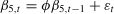
Model specification

This study models the state equation of SED variables as a first-order autoregressive process and the state equation of intervention variables as a random walk process. The TVP-SSM can be defined as follows:

where Yt is the hotel occupancy in Hangzhou, β0 is the intercept; X1,t is tourist flow on Hangzhou Hubin Road, X2,t is passenger arrivals of Hangzhou Xiaoshan International Airport, X3,t is the combined SED variable, Di,t(i=1⋯4) are all dummy variables, including intervention variables and periodical variables. βi,t(i=1,2,3,4) is the dynamic impact of the COVID-19 pandemic and holiday on hotel occupancy; β5,t is the relationship between hotel occupancy and the composite SED variable; ut, ηt and εt are uncorrelated disturbance terms. γ1, γ2 are fixed parameters, reflecting the influence between X1,t, X2,t and Yt, respectively.

Empirical analysis

Model setup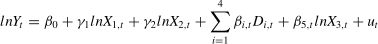

The empirical analysis was carried out on a PC integrated with a Core I9 CPU, 16 G RAM, and the Windows 11 system, and the development environment was EViews 9. The Hangzhou hotel occupancy data set was divided into training and testing sets with a ratio of 743:16. This division ensures that the characteristics of COVID-19 can be captured in both the training and testing phases, allowing the influence of intervention variables on the results to be reflected in the model. Then, 4-step, 8-step, 12-step, and 16-step forward forecasting models were constructed using TVP-SSM-1, ARIMAX, Sequence To Sequence (Seq2Seq), Transformer, multiple linear regression (MLR), support vector regression (SVR), and naïve (NAIVE) models, respectively, to analyze the performance of different models for hotel occupancy prediction. Additionally, to verify the importance of multisource data in hotel occupancy prediction, the TVP-SSM-2, TVP-SSM-3, and TVP-SSM-4 models were constructed. Among them, TVP-SSM-2 only considers official statistics and SED, while TVP-SSM-3 only considers periodic variables, and TVP-SSM-4 only considers SED.

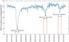
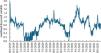
Descriptive analysis

As shown in Fig. 2, there are three troughs (A, B, and C) in the dynamics of daily hotel occupancy in Hangzhou during the covered period. Troughs A and B are due to the influence of the Spring Festival and the COVID-19 pandemic, and trough C is due to the outbreak of the COVID-19 pandemic.

Fig. 2.

Daily hotel occupancy in Hangzhou from October 1, 2019, to October 28, 2021.

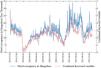
According to Appendix A, keywords with correlation coefficients greater than 0.6 related to hotel occupancy are listed in Table 3. It can be concluded that there is a strong correlation between the retained query keyword volumes and hotel occupancy. The lag order of keyword variables ranges from zero to two, indicating that most relevant queries occur at most two days before the trip. Finally, the volumes of query keywords in Table 3 were normalized and aggregated in the combined keyword variable based on Eqs. (8)–(9). As shown in Fig. 3, the hotel occupancy and combined keyword variable generally exhibited similar fluctuation patterns, particularly in terms of peaks and troughs.

Table 3.

Correlation coefficients between query keyword volumes and hotel occupancy.

Keyword	Correlation Coefficient	Lag Order	Keywords	Correlation Coefficient	Lag Order
Hangzhou food	0.8024	1	Hangzhou tourism	0.6568	1
Hangzhou specialty	0.7648	1	Boat of West Lake	0.6530	2
Hangzhou snacks	0.7573	2	Hangzhou attractions	0.6388	2
Hangzhou Song City	0.6942	1

Fig. 3.

Hotel occupancy and combined keyword variable in Hangzhou.

Model estimation

For econometric models, the results of the stationarity test are shown in Appendix B, and common parameter estimation methods include the least squares method, the maximum likelihood estimation method, etc. Compared to them, the Kalman filter posits that the observed value at the previous time will have an impact on the next time, which is more suitable for the real-time processing of dynamic data (Kalman, 1960). The Kalman filter is an iterative algorithm that continuously estimates and corrects parameters in the state equation based on the Kalman gain according to the difference between the observed value and the actual value.

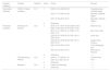
In this study, the Kalman filter is used to estimate the parameters of the TVP-SSM-1. The algorithm is implemented by EViews 9, and convergence is achieved after 118 iterations. Ultimately, the optimal estimated coefficients for the various variables, including SED, COVID-19 state, and holiday variables, are obtained and presented in Table 4.

Table 4.

Results of parameter estimation of TVP-SSM-1.

Variable	Coefficient	Standard error	Z-Statistic	P-value
Intercept	0.4765	0.2759	1.7274	0.0841*
ln(X1,t)	0.3599	0.0203	17.6992	0.0000***
ln(X2,t)	0.6087	0.0164	37.2285	0.0000***
ln(X3,t)	0.4918	0.1223	4.0232	0.0001***
D1,t	−0.0830	0.0243	−3.4153	0.0006***
D2,t	0.0318	0.0420	1.9577	0.0503**
D3,t	−0.1821	0.0466	−3.9064	0.0001***
D4,t	0.0223	0.0195	1.6523	0.0985*

Note: All coefficient estimates are end-state estimates. ***, **, and * represent 1 %, 5 %, and 10 % significance levels, respectively.

According to Table 4, all variables are significant at the 10 % level, suggesting that they are important determinants of hotel occupancy. Among them, official statistics (X1t and X2t), SED (X3t), holiday variables (D2t) and weekends (D4t) show positive effects on hotel occupancy in Hangzhou, while COVID-19 state variables (D1t) and Chinese Spring Festival (D3t) show adverse effects.

During the COVID-19 pandemic, tourism was severely restricted, leading to a significant decline in hotel occupancy and a negative overall impact on the industry. A similar effect was obtained by Ozdemir et al. (2022).

As expected, the impact on hotel occupancy varied by holiday, with occupancy during Labor Day and National Day increasing significantly compared with regular days. On the contrary, hotel occupancy during the Chinese Spring Festival was significantly lower compared with typical days. These patterns were also noted by Liu et al. (2022); however, they have specific differences depending on the destination.

Simulating the impact of dummy variables on hotel occupancy

TVP-SSM-1 updates the coefficients in real time using a Kalman filter, which allows it to capture the dynamic impacts of intervention and periodic variables on hotel occupancy in Hangzhou at different stages, ensuring that these effects align with real-world conditions.

• (1). Impact of intervention variable on hotel occupancy

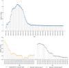
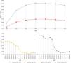
The impact of the COVID-19 pandemic on hotel occupancy in Hangzhou during the three phases is presented in Fig. 4. Among them, subfigure (a) in Fig. 4 indicates that during the comprehensive outbreak stage, the pandemic’s influence on Hangzhou’s hotel occupancy rate initially increased and then decreased. As the pandemic began to spread rapidly across the country, people’s travel was severely restricted, leading to a significant decline in hotel occupancy rates, with the impact steadily increasing over time. From mid to late February 2020, the impact reached its peak, indicating the most substantial effect on hotel occupancy rates. Subsequently, with the effectiveness of a series of domestic prevention and control measures, the influence began to decline and gradually stabilized after March 23, 2020.

Fig. 4.

Impact of COVID-19 on hotel occupancy in Hangzhou during three stages.

Subfigures (b) and (c) in Fig. 4 show that the impact gradually wanes during the sporadic outbreak stages Ⅰ and Ⅱ. In both stages, although local outbreaks initially had an impact on hotel occupancy, the timely implementation of prevention and control measures led to a continuous reduction in the impact. There were some minor fluctuations during these periods, but the overall tendency was a decrease in the impact. This suggests that in the face of sporadic outbreaks, preventive and control measures can effectively mitigate the adverse effects of the pandemic on the hotel occupancy rate, reducing both the scope and degree of impact.

• (2). Impact of periodical variables on hotel occupancy

Given that the holiday effect of longer vacations on hotel occupancy is more realistic, this study analyzes the impact of two of China’s most important traditional holidays: National Day and the Spring Festival.

Subfigure (a) in Fig. 5 shows that during National Day in 2020 and 2021, the impact of holiday effects on hotel occupancy in Hangzhou first increased and then decreased. Among them, October 3 was the most affected, with the highest hotel occupancy. Additionally, the impact of National Day on hotel occupancy in 2020 was significantly higher than that of 2021, mainly because transmission of the COVID-19 pandemic was controlled during National Day in 2020. It was more convenient for tourists to travel, which led to a “revenue spending” trend in the tourism industry. However, the pessimistic situation of the pandemic during the National Day of 2021 reduced hotel occupancy in Hangzhou.

Fig. 5.

Impact of holiday effects on hotel occupancy in Hangzhou.

Subfigures (b) and (c) in Fig. 5 present the impact of the Spring Festival effect on hotel occupancy in Hangzhou for the Spring Festival during 2020 and 2021, respectively. The impact of the Chinese New Year effect generally shows a decreasing trend. In these two figures, the impact stays at a high level in the week before the Chinese New Year and falls back quickly in the week after the Chinese New Year. Comparing 2020 and 2021, it is found that there is no significant difference in the impact of the Spring Festival on hotel occupancy in Hangzhou.

Strategies for forecasting and comparative experiments

The strategy for prediction is to re-estimate the model by adding one day to the forecasting horizon. Ultimately, we obtain 13 four-step-ahead forecasts, nine eight-step-ahead forecasts, five twelve-step-ahead forecasts, and one sixteen-step-ahead forecast. For the out-of-sample prediction, the lagged actual values of SED were used.

To verify the performance ability of the proposed model, two groups of comparative experiments were constructed. In the first experiment, the forecasting results of the TVP-SSM-1, TVP-SSM-2, TVP-SSM-3, and TVP-SSM-4 were compared to demonstrate whether the inclusion of multiple source data, such as intervention variables and periodic variables, could improve prediction accuracy. In the second experiment, to verify the higher prediction accuracy of TVP-SSM-1, the forecasting results of TVP-SSM-1 with ARIMAX, Seq2Seq, Transformer, MLR, SVR, and NAIVE models are compared. In these two experiments, the treatment of other parts remained the same, except for the use of different forecasting models.

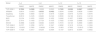
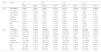
Error analysis

The results of RMSE and MAPE for different models, presented in Table 5, show that the four-step-ahead forecast (h=4) of TVP-SSM-1 has the smallest MAPE of 0.038, and the sixteen-step-ahead (h=16) forecast of TVP-SSM-1 has the smallest RMSE of 0.6967. Compared to TVP-SSM-2, the RMSE and MAPE for TVP-SSM-1 are lower across all forecasting horizons. The inclusion of intervention variables increases the average RMSE and MAPE by 74 % and 76 %, respectively. Compared with TVP-SSM-3 and TVP-SSM-4, the average RMSE and MAPE rise by 93 % and 92 %, respectively. This suggests that the use of multisource data, such as intervention variables, may significantly improve the prediction accuracy. Additionally, the RMSE and MAPE for the TVP-SSM-1 are smaller than those for the ARIMAX, Seq2Seq, Transformer, MLR, SVR, and NAIVE models across different forecasting horizons. Especially compared with the NAIVE model, the average prediction accuracy of TVP-SSM-1 (as measured by the RMSE and MAPE) is higher by 86 % and 87 %, respectively.

Table 5.

RMSE and MAPE for different models and forecasting horizons.

Model	h=4		h=8		h=12		h=16
	RMSE	MAPE	RMSE	MAPE	RMSE	MAPE	RMSE	MAPE
TVP-SSM-1	0.7804	0.0388	1.0228	0.0523	0.7420	0.0389	0.6967	0.0339
ARIMAX	0.8614	0.0453	0.9335	0.0492	0.9244	0.0489	0.8636	0.0464
Seq2Seq	5.2250	0.3080	5.2197	0.3076	5.2228	0.3079	5.2193	0.3076
Transformer	6.9519	0.4125	6.9465	0.4122	6.9530	0.4126	6.9414	0.4118
MLR	3.0154	0.1655	3.0020	0.1652	3.0492	0.1657	2.9698	0.1623
SVR	2.7914	0.1440	2.7724	0.1435	2.7832	0.1436	2.8068	0.1463
NAIVE	6.3988	0.3238	5.6382	0.3005	5.7615	0.3125	5.2666	0.2800
TVP-SSM-2	3.0707	0.1658	3.2791	0.1847	2.9292	0.1618	2.9144	0.1634
TVP-SSM-3	13.9031	0.7955	13.9026	0.7954	13.903	0.7955	13.9015	0.7952
TVP-SSM-4	7.7029	0.3417	8.4239	0.3494	10.197	0.3915	8.5094	0.3552

Note: The best statistical scores are marked in boldface.

The DM statistics in Table 6 indicate that the DM test rejects the null hypothesis at varying levels of significance. Compared with the ARIMAX model, the DM test is positive when h=8.The reason is that the RMSE and MAPE values of the TVP-SSM-1 model are higher than those of the ARIMAX model (see Table 5); however, the difference may be negligible. Whereas the RMSE and MAPE values of the TVP-SSM-1 model are lower than those of the ARIMAX model when h=4,12,16. Compared with the other five models, the TVP-SSM-1 shows significantly superior prediction results. Hence, it is reasonable to conclude that TVP-SSM-1 performs better.

Table 6.

DM test based on RMSE and MAPE for comparing TVP-SSM-1 against competing models with different forecasting horizons.

Competing model	h=4		h=8		h=12		h=16
	RMSE	MAPE	RMSE	MAPE	RMSE	MAPE	RMSE	MAPE
ARIMAX	−2.2401**	−1.9015*	2.1900*	1.8601*	−2.1899**	−1.8586*	−2.1862**	−1.8545**
Seq2Seq	−2.5055**	−3.5600***	−2.3868**	−3.1345***	−2.6330***	−4.6009***	−2.5813***	−4.1168***
Transformer	−3.2841***	−5.0372***	−3.2120***	−4.6004***	−3.3944***	−5.9728***	−3.3584***	−5.6343***
MLR	−4.8874***	−3.9122***	−4.5374***	−2.9850***	−4.2554***	−4.3588***	−3.9578***	−4.1624***
SVR	−2.9902***	−3.9158***	−2.6503**	−2.7344***	−2.9367***	−3.4671***	−3.0304***	−3.6619***
NAIVE	−2.3499**	−3.1836***	−2.4427**	−3.4810***	−2.2922**	−2.8275***	−2.0856**	−2.5881***
TVP-SSM-2	−3.7130***	−2.3675**	−4.1948***	−2.7199***	−2.4399**	−1.8468*	−2.5880***	−1.8466**
TVP-SSM-3	−4.7922***	−6.1003***	−4.7917***	−6.0992***	−4.7921***	−6.1004***	−4.7905***	−6.0964***
TVP-SSM-4	−2.5030***	−3.4181***	−2.8504***	−3.8787***	−3.4108***	−3.7904***	−2.8603***	−3.8948***

Note: ***, **, and * represent 1 %, 5 %, and 10 % significance levels, respectively.

Several factors may explain the high prediction errors observed in the TVP-SSM-2, TVP-SSM-3, TVP-SSM-4, ARIMAX, Seq2Seq, Transformer, MLR, SVR, and NAIVE models. First, the TVP-SSM-2 does not contain intervention variables, and the SED variables alone cannot fully reflect the impact of the pandemic on hotel occupancy. TVP-SSM-3 relies solely on periodic variables; TVP-SSM-4 incorporates only SED data. Second, the ARIMAX model predicts the current value based on historical data, and a lack of shocks in the historical data is likely to inflate the predicted value under the pandemic restrictions. Third, the MLR model is a fixed-parameter model, which cannot dynamically describe the impact of interventions on hotel occupancy. Fourth, although the SVR model can reflect the nonlinear relationship between variables, it cannot accurately learn such a nonlinear relationship because the intervention variables are dummy variables and contain less information than continuous variables. Fifth, the NAIVE models are univariate time series models, making predictions based solely on historical data without the ability to reflect the influence of unexpected external shocks. Sixth, Seq2Seq (Lu et al., 2024) and Transformer (Ma et al., 2023) models are deep learning models that are computationally intensive and time-consuming. These models require massive training data for optimal forecasting performance. Additionally, the impacts of external shocks are unexpected, which may render the patterns learned from the training data inapplicable to the observed samples influenced by external shocks, affecting the accuracy of predictions.

Robustness analysis

In order to further validate the robustness of the TVP-SSM model, three cases are designed: Case 1 changes the ratio of the training set and testing set; Case 2 replaces the response variables; and Case 3 changes the data set. The data set for Hangzhou is utilized in Cases 1 and 2, while Case 3 uses the data set for Zhoushan. The variables and data sets in each case are shown in Table 7.

• Case 1: robustness analysis based on modifying the ratio for data splitting

Table 7.

Variables and data set for robustness testing.

	Case 1	Case 2	Case 3
Data set	Hangzhou Data set		Zhoushan Data set
Response variable	Hotel occupancy in Hangzhou	Revenue of the hotel industry in Hangzhou	Revenue of the hotel industry in Zhoushan
Official statistics	Tourist flow on Hangzhou Hubin Road	Passenger arrivals at Hangzhou Xiaoshan International Airport	Passenger arrivals at Zhoushan Putuoshan Airport
	Passenger arrivals at Hangzhou Xiaoshan International Airport
SED	Baidu Index	Baidu Index	Baidu Index
Intervention variable	COVID-19 state variables	COVID-19 state variables	COVID-19 state variables
Periodical variable	Holidays and festivals	Holidays and festivals	Holidays and festivals
	Weekend	Weekend	Weekend

To verify the robustness of the model, the ratio of the training set to the testing set was categorized into four types (739:20, 743:16, 747:12, and 751:8), and predictions were performed using the settings outlined in Section 5.1.

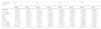
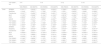
As shown in Table 8, from a horizontal perspective, there are differences in the prediction results of the same model under varying data splitting ratios. Taking TVP-SSM-1 as an example, when the split ratio is 739:20, the MAPE is 0.1306; while when the ratio changed to 743:16, the MAPE is only 0.0319, which indicates that the ratio for data splitting does affect the prediction results; from the longitudinal perspective, the RMSE and MAPE of the TVP-SSM-1 model are smaller than those of the other benchmark models under different ratios for data splitting.

Table 8.

Comparison of RMSE and MAPE under different ratios for data splitting.

Model	739:20		743:16		747:12		751:8
	RMSE	MAPE	RMSE	MAPE	RMSE	MAPE	RMSE	MAPE
TVP-SSM-1	2.3069	0.1306	0.6967	0.0339	0.7855	0.0395	0.9007	0.0502
ARIMAX	2.5375	0.1418	0.8636	0.0464	0.8343	0.0447	1.1469	0.0636
Seq2Seq	5.3053	0.3185	5.2193	0.3076	5.2476	0.3137	4.6211	0.2826
Transformer	6.8578	0.4127	6.9414	0.4118	6.9727	0.4213	6.4974	0.3999
MLR	3.2257	0.1827	2.9698	0.1623	2.9677	0.1676	2.4677	0.1448
SVR	2.8996	0.1474	2.8068	0.1463	2.4986	0.1343	2.3279	0.1236
NAIVE	3.7575	0.1735	5.2666	0.2800	3.8532	0.2044	2.0587	0.0730
TVP-SSM-2	4.0900	0.1969	2.9144	0.1634	2.9292	0.1579	4.4576	0.2343
TVP-SSM-3	14.2192	0.8362	13.9015	0.7952	14.5940	0.8623	13.4078	0.7935
TVP-SSM-4	7.9396	0.3277	8.5094	0.3552	9.5390	0.4022	4.4619	0.2147

Note: The best statistical scores are marked in boldface.

As shown in Table 9, the null hypothesis of the DM test is rejected at the 10 % significance level, indicating a significant difference in the prediction results of the TVP-SSM-1, TVP-SSM-2, ARIMAX, Seq2Seq, Transformer, MLR, SVR, and NAIVE models under different data-splitting ratios. Additionally, all the DM statistics are negative, which further indicates that the TVP-SSM-1 model has better prediction accuracy than the benchmark models. However, it is worth noting that at 8 and 12 steps, the DM test results of TVP-SSM-1 versus TVP-SSM-2 are not significant, mainly because when the forecasting step is short, the TVP-SSM model fails to adequately learn the features of the existing data. The advantages of the time-varying features in the TVP-SSM become evident only when the forecasting horizon is long.

• Case 2: robustness analysis based on different variables

Table 9.

DM test results under different ratios for data splitting.

TVP-SSM-1 VS.	739:20		743:16		747:12		751:8
	RMSE	MAPE	RMSE	MAPE	RMSE	MAPE	RMSE	MAPE
ARIMAX	−2.8958***	−3.9648***	−2.0800**	−2.4146**	−3.2655***	−3.2147***	−2.6907**	−2.4873**
Seq2Seq	−2.6044***	−3.7653***	−2.5813***	−4.1168***	−2.2139**	−3.1417***	−2.5410**	−2.8445***
Transformer	−3.2268***	−5.0700***	−3.3584***	−5.6343***	−3.1802***	−4.6624***	−5.0445***	−4.3880***
MLR	−3.7276***	−2.5694**	−2.9931***	−2.4052**	−2.8027***	−3.5838***	−3.0104***	−3.0938***
SVR	−4.4316***	−3.3288***	−2.2337**	−2.4246**	−2.6008**	−2.7420**	−3.8739***	−3.8734***
NAIVE	−1.7864*	0.1950	−2.0856***	−2.5881***	−1.7243*	−2.1131**	−2.6505***	−3.8839***
TVP-SSM-2	−1.8970*	−1.6868	−2.5880***	−1.8466*	−0.7561	−1.2223	−1.2076	−1.1410
TVP-SSM-3	−5.0431***	−7.3936***	−4.7905***	−6.0964***	−5.219***	−5.5319***	−4.8028***	−5.9891***
TVP-SSM-4	−3.511***	−3.9736***	−2.8603***	−3.8948***	−3.5505***	−3.9756***	−2.7757***	−2.1737**

Note: ***, **, and * represent 1 %, 5 %, and 10 % significance levels, respectively.

In Case 2, the revenue of the hotel industry in Hangzhou is regarded as the response variable. A forecasting model is then constructed, and it is verified that the TVP-SSM exhibits an excellent predictive effect for different response variables.

Appendix C demonstrates the significant correlation and causality between hotel consumption in Hangzhou and passenger arrivals of Hangzhou Xiaoshan International Airport (X2,t) and composite SED variable (X3,t), which further validates the reasonableness of using passenger arrivals of Hangzhou Xiaoshan International Airport (X2,t) and composite SED variable (X3,t) to predict hotel consumption in Hangzhou.

The average values of RMSE and MAPE for the TVP-SSM-1 model are 0.2127 and 0.0685, respectively, and these values are significantly smaller than those of the other benchmark models at different prediction steps, indicating that the TVP-SSM model performs well. Additionally, the DM statistics of Case 2 in Table 10 are all negative, indicating that the prediction results of TSVP-SSM-1, TSVP-SSM-2, ARIMAX, Seq2Seq, Transformer, MLR, SVR, and NAIVE models are significantly different under different prediction steps. The prediction accuracy of the TSVP-SSM-1 model is higher than that of other benchmark models.

• Case 3: robustness analysis based on Zhoushan data set

Table 10.

Comparison of RMSE and MAPE at different prediction steps.

Case	Model	h=4		h=8		h=12		h=16
		RMSE	MAPE	RMSE	MAPE	RMSE	MAPE	RMSE	MAPE
Case 2	TVP-SSM-1	0.1923	0.0611	0.2289	0.0732	0.2172	0.0708	0.2123	0.0687
	TVP-SSM-2	1.4781	0.4052	1.9013	0.6182	2.2395	0.7203	2.2907	0.8077
	TVP-SSM-3	1.3809	0.4915	1.3808	0.4913	1.3807	0.491	1.3807	0.491
	TVP-SSM-4	0.3205	0.082	0.3203	0.082	0.3206	0.082	0.3204	0.082
	ARIMAX	0.2776	0.0801	0.2910	0.0913	0.2934	0.0893	0.2886	0.0835
	Seq2Seq	0.7765	0.2797	0.7750	0.2791	0.7760	0.2794	0.7751	0.2790
	Transformer	2.3946	0.8938	2.3930	0.8933	2.3906	0.8924	2.3814	0.8890
	MLR	0.3588	0.1141	0.3583	0.1138	0.3588	0.1141	0.3602	0.1147
	SVR	0.3198	0.0956	0.3345	0.1054	0.3324	0.0995	0.3245	0.0912
	NAIVE	0.7664	0.1918	0.5968	0.1564	0.5748	0.1695	0.5070	0.1331
Case 3	TVP-SSM-1	174.5994	0.0524	162.2061	0.0424	174.4974	0.0504	161.4568	0.0447
	TVP-SSM-2	1003.7645	0.3224	2045.5378	0.6278	2432.6180	0.7000	2780.6212	0.8590
	TVP-SSM-3	2573.4767	0.8265	2573.0678	0.8262	2572.3978	0.8257	2572.3978	0.8257
	TVP-SSM-4	1389.6447	0.3207	1418.5824	0.3237	932.4355	0.2521	1408.0734	0.3223
	ARIMAX	184.1614	0.0648	234.4958	0.0560	281.1958	0.0683	271.2229	0.0615
	Seq2Seq	1318.0825	0.4225	1318.7672	0.4228	1319.7890	0.4231	1319.4584	0.4230
	Transformer	1562.1517	0.4355	1564.5224	0.4368	1562.5534	0.4358	1563.4481	0.4363
	MLR	772.7561	0.2453	770.2594	0.2444	772.9813	0.2450	777.3334	0.2468
	SVR	188.1767	0.0821	245.3478	0.0701	282.1134	0.0845	280.4156	0.0713
	NAIVE	809.2093	0.2034	665.9044	0.1707	818.8434	0.1985	741.2329	0.1831

Note: The best statistical scores are marked in boldface.

Further, in order to verify the fitting effect of the TVP-SSM model on different data sets, robustness analysis was carried out based on the Zhoushan data set in Case 3. Considering the potential heterogeneity in the Zhoushan dataset, the search engine variables, intervention variables, and periodical variables were processed according to Section 4. Subsequently, correlation and causality tests among these variables were conducted, as shown in Appendix D.

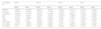
As shown by the results of Case 3 in Table 11, for hotel consumption prediction in Zhoushan, the TPP-SSM-1 model achieves an average RMSE of 168.1899 and an average MAPE of 0.0475, both of which are significantly lower than those of the benchmark models across different prediction steps, indicating that the TPP-SSM-1 model demonstrates strong predictive performance. Additionally, the DM test results of Case 3 in Table 11 show that the prediction results of TPP-SSM-1, TPP-SSM-2, ARIMAX, Seq2Seq, Transformer, MLR, SVR, and NAIVE models are significantly different under different prediction steps, and the prediction accuracy of the TVP-SSM model is higher than that of these benchmark models.

Table 11.

DM test results under different prediction steps.

	TVP-SSM-1, VS.	h=4		h=8		h=12		h=16
		DM (RMSE)	DM (MAPE)	DM (RMSE)	DM (MAPE)	DM (RMSE)	DM (MAPE)	DM (RMSE)	DM (MAPE)
Case	ARIMAX	−2.1911***	−2.9418***	−2.5531**	−2.6532***	−2.7665***	−3.3523***	−3.4509***	−3.4131***
	Seq2Seq	−1.9146*	−2.5677**	−1.7326*	−1.9795**	−1.8761*	−2.4055**	−1.8466*	−2.2898**
	Transformer	−3.0127***	−3.4450***	−3.0062***	−3.4251***	−3.0148***	−3.4219***	−3.0611***	−3.4797***
	MLR	−3.1305***	−3.3946***	−3.1344***	−4.1023***	−3.9578***	−4.1624***	−3.1305***	−3.3946***
	SVR	−2.0839**	−1.8142*	−2.0515**	−1.7793*	−2.0502**	−1.7769*	−2.0468**	−1.7731*
	NAIVE	−1.9130*	−2.4131**	−1.8952*	−2.2027**	−2.7862***	−3.2321***	−3.4246***	−3.7993***
	TVP-SSM-2	−1.0747	−1.7404*	−1.7117*	−2.1586**	−1.8159*	−2.4478**	−2.1328**	−2.7868***
	TVP-SSM-3	−1.7075*	−2.0134**	−1.7066*	−2.0108**	−1.7049*	−2.0036**	−1.7049*	−2.0036**
	TVP-SSM-4	−2.3055**	−2.1904**	−3.3054***	−2.1909**	−3.3058***	−2.1904**	−3.3055***	−3.191***
	ARIMAX	−1.7227*	−1.6761*	−1.7507*	−1.6651*	−2.2379**	−1.8374**	−1.7227*	−1.676*
	Seq2Seq	−3.5978***	−8.6120***	−3.6758***	−8.3124***	−3.6125***	−8.2378***	−3.6442***	−8.2014***
	Transformer	−1.0297	−2.2951**	−1.0379	−2.3884**	−1.0307	−2.2836**	−1.0357	−2.3697**
	MLR	−4.5929***	−4.0273***	−3.7254***	−5.0457***	−3.0304***	−3.6619***	−4.5929***	−4.0273***
	SVR	−4.1116***	−2.8682***	−2.8006***	−2.0014**	−2.3089**	−1.6709*	−4.1116***	−2.8682***
	NAIVE	−3.9792***	−9.1126***	−0.8055	−5.1350***	−0.8508	−4.9516***	−0.7630	−5.6605***
	TVP-SSM-2	−5.1342***	−3.8830***	−1.1579	−2.1761**	−1.5080	−2.0049**	−1.6552*	−2.1625**
	TVP-SSM-3	−2.0729**	−2.5748**	−2.0700**	−2.5702**	−2.0651**	−2.5615**	−2.0651**	−2.5615**
	TVP-SSM-4	−2.5047**	−2.9343***	−2.4847**	−2.9195***	−2.0979**	−2.3456**	−2.4889**	−2.9202***

Note: ***, **, and * represent 1 %, 5 %, and 10 % significance levels, respectively.

Discussion

In this study, we propose a hotel occupancy prediction framework that incorporates multisource data. The study finds that multisource data can effectively improve the accuracy of hotel occupancy predictions, consistent with Pan and Yang (2016). The main reason is that multisource data reflect tourists’ behavioral characteristics from multiple dimensions. For example, SED reflects tourists’ perceptions of tourist destinations through search keywords, so different search keywords are crucial to the model results. Additionally, the Baidu search index exhibits higher precision in forecasting tourism demand for the Chinese market (Yang et al., 2015). The holiday variable reflects the strong demand for tourism. Generally speaking, holidays are the peak of tourism, and scenic spots and hotels are full (Bi et al., 2021; Liu et al., 2018). Official high-frequency statistics, such as airport passenger flow, reflect tourist behavior (Liu et al., 2022), which is also a significant advantage of this paper compared with other studies. Therefore, integrating multivariate data can effectively enhance the performance of the prediction model.

Second, it has been shown that external intervention events, such as terrorist attacks (Toma et al., 2009) and stock and economic crises (Eugenio-Martin, 2016), have an impact on tourism demand forecasting. In this paper, COVID-19 is regarded as an external intervening variable. The TVP-SSM model is employed to capture the effects of external intervening variables on hotel occupancy. It adjusts model coefficients in real time using Kalman filtering, allowing it to reflect the dynamic impacts of these variables on occupancy across different stages, aligning the shocks with actual conditions.

However, this study exhibits certain limitations that should be taken into account. First, the study only considers the search volume of tourists on the Baidu platform. In fact, many tourists may choose Google, Weibo, Airbnb, and other online platforms for trip planning. Therefore, combining multimodal data may further improve prediction accuracy (Tan et al., 2025). Second, this paper focuses solely on Hangzhou and Zhoushan as case studies. Given the differences in coping strategies adopted by different regions in the face of external shocks, the performance of the model proposed in this study may fluctuate in tourist forecasting scenarios in different regions, and future work can focus on inter-regional heterogeneity. Third, the COVID-19 pandemic is regarded as an external shock and is represented by a dummy variable with only two values (0 and 1). However, in fact there are many types of external shock events that affect tourist flow with diverse degrees of impacts. The application of the model proposed in this study can be discussed separately for these different types of impact factors in the future.

Conclusion and discussion

Conclusion

A TVP-SSM model was constructed in this study, which included the official statistics, SED, intervention variables, and periodical variables. The model was applied to generate short-term predictions of daily hotel occupancy in Hangzhou under the impact of external events, such as the COVID-19 pandemic. The empirical results show that (1) During the comprehensive outbreak stage of the COVID-19 pandemic, the adverse effect of COVID-19 on hotel occupancy increased rapidly at first and then decreased gradually. In the subsequent sporadic outbreak stage, the pandemic situation and restrictions would also decrease hotel occupancy. (2) Adding interventions and SED to the estimation can significantly boost the prediction accuracy. (3) Overall, the TVP-SSM model, incorporating intervention and periodic variables, demonstrated strong performance in forecasting hotel occupancy, effectively capturing the impact of external shocks.

The results of this study have significant implications for hotel operations and management, offering tourism and hospitality industry decision-makers a new approach to emergency scenarios. Specifically, the proposed approach enables the tracking of tourist flows in the short term and ensures that forecasting includes the most recent data without incurring a significant cost increase. Meanwhile, the results can help operators to develop pricing strategies that consider the expected tourism demand. Tourism operators can develop contingency plans to manage fluctuations in tourist flow during specific periods.

Moreover, this paper mainly focuses on analyzing how external intervention variables impact hotel occupancy predictions. To our knowledge, most existing studies on occupancy forecasting primarily utilize time-series data and online metrics, with scant attention paid to intervention factors. However, in reality, sudden disruptions like COVID-19 can have a profound impact on occupancy rates. By systematically examining intervention effects through the integration of multisource data, our work establishes theoretical foundations and offers reference value for future research in this critical direction.

Implications

To evaluate the impact of external events, we propose a new forecasting framework based on multisource data, which holds significant theoretical and practical implications for tourism demand forecasting and management.

First, from a theoretical perspective, external events such as the COVID-19 pandemic make tourism demand forecasting particularly challenging. Hence, based on the TVP-SSM, the forecasting framework constructed in this paper innovatively integrates multiple sources of data, comprehensively reflecting the impact of various factors on tourism demand, which improves the forecasting performance. Additionally, the proposed time-varying model can dynamically simulate the impact of external events on tourism demand, providing solid support for research on tourism demand forecasting under the influence of external events. What is more, the proposed forecasting framework can be extended to analyze the dynamic relations between socio-economic variables, such as the dynamic relations between the relationship between inflation and GDP.

Second, in terms of practical aspects, the results of this study have important implications for hotel business management, providing tourism and hospitality industry decision-makers with a new approach for emergency scenarios. Specifically, the proposed approach allows tourist flows to be tracked in the short run. It can ensure that the forecasting models include the most recent data without a serious cost increase. Meanwhile, the results can help operators to conduct pricing strategies that consider the expected tourism demand. Tourism operators can develop contingency plans to manage fluctuations in tourist flow during specific periods.

CRediT authorship contribution statement

Ji Chen: Writing – review & editing, Supervision, Resources, Project administration, Funding acquisition, Conceptualization. Kang Tong: Writing – original draft, Visualization, Validation. Qinglin Yu: Writing – original draft, Software, Methodology, Investigation. Sichao Chen: Software, Methodology, Investigation, Formal analysis. Tomas Balezentis: Writing – review & editing, Writing – original draft, Methodology, Conceptualization. Dalia Streimikiene: Writing – review & editing, Validation, Investigation, Conceptualization.