


This paper examines the impact of the Global Innovation Index (GII) and uncertainty and of their interaction on bank performance in the Middle East and North Africa (MENA) from 2011 to 2022. Our findings indicate that innovation is associated with nuanced relationships with bank performance indicators, and innovation potentially increases (decreases) performance via the return on asssets (ROA), return on equity (ROE), Tobin’s Q, and stock market returns. Our analysis demonstrates that uncertainty plays a complex role in influencing bank performance. It has a negative impact on economic policy uncertainty (EPU) and the World Uncertainty Index (WUI), but a positive impact on geopolitical risk (GPR). However, we observe an interaction effect, which suggests that uncertainty has the potential to either diminish or amplify the impact of innovation on bank performance metrics. Specifically, the relationship between innovation and bank performance, whether negative or positive, is influenced by the presence of uncertainty. This nuanced interaction highlights the dynamic nature of the relationship between innovation and bank performance, as it is contingent on the prevailing level of uncertainty. Therefore, fostering an environment in the banking sector that is conducive to growth and stability is crucial for enhancing innovation, minimizing uncertainty, and improving bank performance.
A national innovation system (NIS) is a conceptual framework on how public and commercial entities collaborate to stimulate the development and diffusion of new technologies in a country. The core idea of this concept is that innovation and technological progress are influenced by dynamic interactions among different actors (Freeman, 1987; B. A. Lundvall, 1992). It evaluates several facets of an economy’s innovation ecosystem. Rooted in the NIS, the Global Innovation Index (GII) is a metric that assesses a country’s potential and efficiency in terms of innovation by considering inputs and outputs (Nyssen Guillén & Deckert, 2021). Inputs are the components of the economy that support innovative activity, whereas outputs are the results of innovative activity over a specific timeframe (Cornell University, INSEAD, & WIPO, 2020).
Since its inception, the GII has attracted academic attention for assessing the comparative innovation capabilities of countries. The GII dataset has been used in numerous studies to investigate different facets of national innovation (Al-Sudairi & Bakry, 2014; Carpita & Ciavolino, 2017; Jankowska et al., 2017; Pençe et al., 2019; Reis et al., 2018; Sohn et al., 2016). Intuitively, on a small scale, firms can enter markets, expand their market share, surpass competitors, and improve profitability through innovation (Blanco & Goel, 2023). Recent studies provide substantial evidence regarding the crucial role of innovation, digital adoption, and financial technology in shaping the current economic and financial environment (Appio et al., 2021; Di Vaio et al., 2021). For example, some studies have shown that these elements play a substantial role in increasing corporate performance (Dhiaf et al., 2022), driving financial success (Siska, 2022), and enhancing economic productivity (Song & Appiah-Otoo, 2022).
Innovation is a multidimensional term that is influenced by various elements, not just technological improvements (Carlsson & Stankiewicz, 1991). The function of institutions in driving innovation is crucial. Effective institutions focus on the amount and quality of social connections and promote the integration of research benefits or external influences. Institutions have been crucial in fostering innovation by implementing patent policies in this vast domain. Better institutional quality can influence the time and distribution of resources dedicated to innovation, thereby enhancing the efficiency of innovation output (Blanco & Goel, 2023). The technical innovation system emphasizes the interconnection among digital technology adoption, the innovation process, and the field of financial technology (fintech) (Carlsson & Stankiewicz, 1991). Hussain and Papastathopoulos (2022) argue that combining digitization and financial innovation facilitates the rapid adoption of digital technologies, leading to better financial performance and firm resilience.
Likewise, global innovation is crucial for banking sector performance. Some studies have demonstrated a correlation among financial innovation, green finance, and sustainability performance, indicating their potential to stimulate sustainable growth (Hussain et al., 2023). Yoon, Lee, and Oh (2023) document that fintech levels prioritize bank performance as a gauge of innovation, especially in emerging economies. The introduction of innovative technologies, such as automatic teller machines and internet banking, has a beneficial impact on the financial performance of banks. The implementation of point-of-sale systems also has a significant impact on the operational performance of banks. Forcadell et al. (2019) note that service innovation performance positively impacts corporate sustainability in the banking business. In addition, the banking sector has been influenced by innovation and evolving financial conditions, which have emerged as critical catalysts for change. Notably, advancements such as mobile banking, internet banking, and agency banking have substantially impacted financial performance (Nyamekye et al., 2023). Incorporating artificial intelligence, data science, and blockchain technology has significantly altered the worldwide financial services industry (Shrier & Pentland, 2022). Moreover, technological progress has resulted in contactless credit and debit cards, which employ near-field communication technologies to make transactions more convenient (Mororó et al., 2023).
However, the financial industry has faced substantial difficulties due to worldwide uncertainty. The COVID-19 pandemic led to a severe economic downturn, which created a high level of uncertainty in the global banking system. This situation shows the need to comprehend the evolving role of financial intermediaries in enabling the effective allocation of capital and promoting economic growth (Huang et al., 2023). Ubilava (2019) states that financial uncertainty directly impacts overall economic performance, particularly during periods of stress. Country-specific uncertainty influences cross-border banking flows by functioning as a push and pull factor, reducing outflows and inflows (Choi & Furceri, 2018). Banks, when vulnerable to financial crises, favor steady profit-creation models and implement effective tactics to achieve banking performance (Harangus, 2012). Adopting digital technologies as a component of disruptive technologies can boost organizations’ technical and social innovative capacities in uncertain conditions, which enables organizations to mitigate challenges linked to a decline in business cycles.
Prior research investigating the correlation among innovation, bank performance, and profitability has concentrated chiefly on innovation’s financial, product, and operational aspects. Innovation in the corporate world, workplace, and external interactions involves implementing new products, processes, marketing tactics, and organizational approaches. This notion includes the creation of new ideas and the merging of existing ones. However, innovations do not occur in isolation. Institutional frameworks, support activities, and infrastructure impact innovation activities and economic growth. The concept used to encompass this is NIS: the processes through which novel technologies are generated, obtained, modified, and disseminated by both public and private entities (Freeman, 1988). NIS prioritizes a collaborative network of universities, government entities, and individual enterprises, rather than focusing solely on the activities of individual firms (Metcalfe & Ramlogan, 2008; Watkins et al., 2015). Nelson (1993) and B. A. Lundvall (1992) proposed the notion of an NIS as a cohesive framework in which institutions, networks, and policies collaborate to promote technological innovation. Some studies propose that innovations can modify investment patterns and risk assessment systems in the financial sector (Lazonick, 2005; Mazzucato, 2013). Hence, this study examines the role of global innovation and uncertainty on bank performance in the Middle East and North Africa (MENA) region as well as the impact of the interaction between global innovation and uncertainty on bank performance.
This paper contributes to the literature on bank performance in three ways. First, to the best of our knowledge, it is the first study that analyzes the role of macrolevel, multidimensional innovation—captured by the GII—in shaping bank performance across the MENA region. In doing so, it goes beyond the dominant focus in prior studies on microlevel, firm‑specific innovation (e.g., Beck et al., 2016; Lee et al., 2021; Li et al., 2022) to fill a critical gap in understanding about how national and systemic innovation environments affect the banking sector. Second, this paper provides a nuanced examination of the interaction between innovation and uncertainty and its impact on bank performance in a region marked by significant economic and political volatility. The interplay between the GII and measures of uncertainty—economic policy uncertainty (EPU), geopolitical risk (GPR) and the World Uncertainty Index (WUI)—has been largely overlooked in the literature, especially in the MENA context, in which institutional constraints and external shocks can profoundly affect bank stability and growth. Third, this study uses a quantile regression approach, which enables a more nuanced assessment of bank performance across its distribution, capturing heterogeneity between low‑ and high‑performing banks. By going beyond traditional mean‑based analyses, this approach provides deeper insights into how macrolevel innovation and uncertainty dynamics operate differently across banks with varying characteristics, yielding more robust and actionable results for both researchers and policy makers. Together, these contributions deepen our understanding of the complex interplay among innovation, uncertainty, and bank performance, offering valuable evidence for researchers, regulators, and bank managers who seek to foster more resilient financial systems in the MENA region.
After this introduction, the paper is structured as follows. Section 2 reviews the literature on the influence of innovation and uncertainty on bank stock returns. In Section 3, the methodology, data, and variables are described, as well as the development of our hypotheses. In Section 4, the empirical findings are analyzed and discussed. Section 5 gives our conclusion.
Literature reviewPrevious studies that examine the intersection of innovation, uncertainty, and bank performance have predominantly focused on specific dimensions of innovation, such as financial, product, and operational aspects. A broader definition of innovation encompasses the implementation of new ideas and recombining existing ones, but the discussion often centers on individual firms’ efforts. However, when considering the NIS, we widen the perspective further. The NIS framework, introduced by Nelson (1993) and B. A. Lundvall (1992), shifts the focus from individual firms to an interdependent system that includes not just individual firms but university and government actors (Metcalfe & Ramlogan, 2008; Watkins et al., 2015). This collaborative approach highlights the influence of institutional structures, support activities, and infrastructure on innovation activities and economic growth (Lazonick, 2005; Mazzucato, 2013).
Bank sector profitability, measured by indicators such as the return on assets (ROA) and return on equity (ROE), is strongly correlated with an innovation-driven environment (Cui et al., 2021; Khan, 2022; Norsalehe & Idris, 2022). Schumpeter’s theory posits that innovation-driven economies will likely enhance financial performance, improving asset quality, reducing default risk, and creating a dynamic business environment (Beck et al., 2016). However, this relationship is not uniformly positive. Research grounded in the innovation-fragility perspective and the “dark side” of innovation literature suggests that, although innovation can increase efficiency, it can also increase systemic risk and instability, as seen during the global financial crisis (Brunnermeier, 2009; Gennaioli et al., 2012; Laeven, Ratnovski, & Tong, 2016). In addition, the “dark side” of innovation has been explored, linking corruption to a distrust of market institutions, hindering firms’ innovative activities (Anokhin & Schulze, 2009; Paunov, 2016). However, efforts to combat corruption have been associated with increased R&D investment, patent generation, and encouragement of innovation (Xu & Yano, 2017).
The literature also emphasizes the role of innovation in the growth of firms, particularly in developed economies, in which firms adjust strategies based on environmental learning (Fu et al., 2018; Geroski, 1989; Klepper, 1996). However, innovation becomes a crucial component of survival at firms in developing countries with poor infrastructure and limited resources (Fagerberg et al., 2010). This aligns with institutional theory, which highlights the role of country-specific institutional quality and governance in shaping how innovation is translated into outcomes. In the MENA region, institutional weakness and regulatory constraints can hinder or distort the innovation-performance relationship (World Bank., 2019).
The theory of constraint-induced financial innovation (Silber, 1983) argues that excessive regulation leads banks to avoid experimentation and innovation. Removing these constraints becomes a prerequisite for innovation-led performance. In contrast, the dynamic capabilities theory (Teece, Pisano, & Shuen, 1997) posits that firms, including banks, that have strong internal learning and adaptive capabilities can harness innovation even under institutional or regulatory pressure.
EPU concerns policy makers and financial institutions. The impact of EPU on bank profitability and performance is analyzed using various economic theories. Institutional theory reveals that MENA’s weak financial institutions amplify the harmful effects of uncertainty on banks, leaving them more exposed to shocks than mature markets (Donker et al., 2020). Agency theory posits that, in times of uncertainty, managers might prioritize short-term gains over long-term profitability, leading to risk aversion and cash retention (Wang et al., 2014).
The real options theory suggests that firms might delay or reduce investment during periods of high economic uncertainty to avoid costly mistakes (A. K. Dixit & Pindyck, 1994; Gulen & Ion, 2016). Borrowers, managers, and investors face information asymmetry, reducing loan amounts during periods of high uncertainty (Çolak et al., 2017). Banks, particularly larger ones, experience lower credit growth during times of uncertainty (Hu & Gong, 2019).
Bank performance and profitability are influenced by uncertainty through increased risk aversion, higher borrowing costs, and lower consumer confidence (Billings et al., 2020; Donker et al., 2020; Lewellen, 2006; Su et al., 2023). In this sense, macroeconomic uncertainty interacts with institutional weakness to create systemic vulnerability, particularly in developing and emerging markets such as the MENA region (Akinci & Olmstead-Rumsey, 2018; IMF, 2021).
The dynamic nature of the banking industry shows the importance of innovation in performance and competitiveness. However, the relationship between innovation and bank profitability becomes more complex when uncertainty is a significant moderating factor. This review uses established theoretical frameworks, namely Schumpeter’s growth theory, real options theory, institutional theory, agency theory, dynamic capabilities theory, and constraint-induced innovation theory, to explore the interaction among innovation, uncertainty, and bank profitability in stable and volatile environments.
The real options theory suggests that uncertainty enables banks to delay or abandon innovation investment until they achieve greater clarity about the benefits and risks. Although this delay mitigates the negative impact of uncertainty on profitability, it might hinder the benefits associated with successful innovation (Adra et al., 2023; Kogut & Kulatilaka, 2001). As a result of uncertainty, firms may be more cautious about making investment decisions and may value waiting. Firms cannot redeploy or recover an investment without financial loss if an investment is irreversible. As a result, minimizing irreversible investment and increasing flexibility are prudent decisions when the company faces high uncertainty (Huang et al., 2023).
The current literature provides rich but often fragmented insights into the effect of innovation and uncertainty on bank performance. Our study contributes to this body of work by empirically exploring how NIS and multiple dimensions of uncertainty jointly shape bank profitability in the MENA region. This underexplored context enables a more nuanced understanding of the interaction between institutional and innovation-related factors under real-world constraints.
Although previous studies have investigated the impact of uncertainty and some elements of NIS on bank performance, a notable gap exists with regard to interaction between NIS and uncertainty. Most studies have focused on financial innovation, but have not exported the interplay between NIS and uncertainty.
Zhang et al. (2022) investigate the combined effect of uncertainty and governance on bank performance, finding that strong risk governance substantially reduces the effects of economic uncertainty on bank performance and risk.
To address this gap, we examine interaction between the GII and uncertainty on bank profitability in the MENA region, contributing to a more nuanced understanding of the factors that influence bank performance in the face of uncertainty. Most studies on the relationship between innovation and bank performance have focused on microlevel, firm-specific innovation, leaving a gap about how macrolevel innovation systems, such as NIS, influence bank performance. Although the impact of uncertainty on bank performance has been analyzed, few studies explore its interaction with innovation, particularly in regions such as the MENA, which are characterized by great economic and political uncertainty. In addition, little research has been conducted on the role of governance mechanisms and regulatory reforms in mitigating the negative effects of uncertainty and fostering innovation in the banking sector. Prior papers also often overlook regional nuances, especially in developing regions such as MENA, in which institutional frameworks and economic conditions differ markedly from those in developed economies. Furthermore, the dynamic interplay between NIS and uncertainty is underexplored despite its potential to significantly shape bank performance, highlighting the need for a more comprehensive investigation of these factors. Table 1 summarizes our review of the literature.
Summary of the empirical literature review.
| Article | Objective/Purpose | Method | Results | Key Insight/Relevance |
|---|---|---|---|---|
| Zhang et al. (2022) | The combined effect of uncertainty and governance on bank performance. | Empirical study using governance metrics and economic uncertainty indexes. | Strong risk governance substantially reduces the negative effects of economic uncertainty on bank performance and risk. | Key contribution: Validates our combined GII-uncertainty-governance approach. |
| Cui et al. (2021) | Correlation between innovation-driven environments and bank profitability (ROA, ROE). | Empirical analysis using financial data from banks. | Innovation-driven environments enhance bank profitability by improving asset quality, reducing default risks, and fostering a dynamic business environment. | Supports the inclusion of GII in our model by highlighting the role of macrolevel innovation environments in bank profitability, a gap in MENA-focused studies. |
| Xu & Yano (2017) | Anticorruption efforts and innovation. | Quantitative analysis of R&D investment and patent generation. | Anticorruption efforts are associated with increased R&D investment, patent generation, and innovation encouragement. | Policy implication: Supports our regulatory reform recommendations. |
| Beck et al. (2016) | Schumpeterian theory: Innovation’s impact on financial performance. | Theoretical framework with empirical evidence. | Innovation enhances financial performance by driving economic growth and reducing risks. | Theoretical anchor: Justifies our use of Schumpeterian framework for MENA banks. |
| Wang et al. (2014) | Agency theory: Managerial behavior during uncertainty. | Empirical analysis of managerial decision-making under uncertainty. | Managers prioritize short-term gains over long-term profitability during uncertain times, leading to risk aversion and cash retention. | Behavioral insight: Explains our bank-level control variables. |
| Fagerberg et al. (2010) | Innovation as a survival mechanism for firms in developing countries. | Comparative analysis of innovation strategies in resource-limited settings. | Innovation becomes critical for survival in developing countries with poor infrastructure and limited resources. | Regional alignment: Justifies our MENA focus where innovation serves survival vs. growth. |
| Anokhin & Schulze (2009) | Corruption’s impact on innovation (“dark side” of innovation). | Empirical study linking corruption to distrust in market institutions. | Corruption hinders firms’ innovative activities due to institutional distrust. | MENA relevance: Explains why we include governance controls in our models. |
| Brunnermeier (2009) | “Innovation-fragility” perspective: Negative effects of financial innovation. | Case study analysis of the global financial crisis. | Financial innovation contributed to systemic risks and the 2008 crisis. | Highlights the need to assess the risk–innovation balance within MENA’s institutional and economic context, especially amid rising uncertainty. |
| A. K. Dixit & Pindyck (1994) | Real options theory: Investment decisions under uncertainty. | Theoretical modeling of investment delays during uncertainty. | Firms delay investment during high uncertainty to avoid irreversible costs, reducing innovation benefits. | Theoretical link: Supports the quantile regression approach used in our study to capture uncertainty thresholds. |
| Smith, Ziehmann, & Fraedrich (1999) | Impact of economic policy uncertainty (EPU) on lending and profitability. | Financial intermediation theory applied to bank behavior. | High EPU discourages lending, reduces credit availability, and lowers profit margins. | Directly informs our approach to capturing EPU–GII interactions and their combined effects on bank performance in MENA. |
| Geroski (1989) | Role of innovation in firm growth, particularly in developed economies. | Environmental learning models and longitudinal data. | Firms in developed economies adjust strategies based on environmental learning, enhancing growth through innovation. | Contextual contrast: Justifies our focus on developing economies (MENA) where innovation dynamics differ. |
| Silber (1983) | Theory of constraint-induced financial innovation. | Theoretical framework analyzing regulatory constraints on innovation. | Regulations hinder innovation in banking; removing constraints is essential for fostering innovation. | Regulatory dynamics: Highlights the tension between financial regulation and innovation, contextualizing our uncertainty measures as potential moderators of GII effectiveness. |
This study evaluates the influence of global innovation and uncertainty on bank performance, both individually and in terms of their interactive effects, in the countries in the MENA region. The sample encompasses publicly traded banks in 20 MENA countries from 2011 to 2022: Algeria, Bahrain, Djibouti, Egypt, Iran, Iraq, Israel, Jordan, Kuwait, Lebanon, Libya, Morocco, Oman, Palestine, Qatar, Saudi Arabia, Syria, Tunisia, the United Arab Emirates, and Yemen. Banks with no data for five consecutive years of the dependent variable are excluded. The final sample consists 5684 observations from 406 banks, comprising 266 conventional and 140 Islamic banks.
The sample data and sample period are chosen in order to explain the economic and financial interconnectedness of countries in the MENA region from 2011 to 2022. Various factors are considered to show their significance and commonality in these countries. First, an evaluation of economic integration is crucial, as it reveals the extent of interconnectedness through trade agreements, economic partnerships, and regional initiatives among MENA countries. Additionally, the degree of financial interdependence plays a pivotal role, encompassing cross-border investment, banking collaboration, and financial market linkages, thereby contributing to shared financial infrastructure and common challenges in the banking sector. Furthermore, exploring energy sector dynamics is important, given the prominent role of many MENA countries in the global energy market. Insights into commonalities in energy policies, production, and export strategies can shed light on shared economic challenges and opportunities. The MENA region is globally distinctive based on its unique financial markets, which rely heavily on bank finance and government ownership, particularly in the region’s oil-exporting countries (Albaity et al., 2023; El Khoury et al., 2023; Mallek et al., 2024). Understanding geopolitical influences is equally vital, considering the region’s complexity, as shared challenges related to geopolitical risk, regional conflicts, and diplomatic relations can significantly impact the stability and performance of banks. As a result of civil unrest and conflicts in several MENA countries in recent years, financial markets, especially the banking sector, have been affected by significant political and social turmoil (Albaity et al., 2021; Mallek et al., 2022). The effects of instability on the banking sector and the broader economy can be determined by exploring bank performance over this period.
Moreover, adopting technology and innovation in the banking industry is a global trend. Assessing the technological adoption and innovation level across MENA countries can illustrate their shared challenges and advancements. Demographic trends, such as population growth rates, the age distribution, and urbanization patterns, have economic implications, requiring adaptation in banking sectors to similar demographic challenges and opportunities.
Finally, understanding how global economic conditions collectively impact MENA countries is crucial in the context of the globalization of financial markets. Shared exposure to global economic trends, such as recessions or economic booms, can significantly affect banking performance. By comprehensively examining these factors, our research identifies the commonalities and assesses the importance of various aspects that shape the economic and financial landscape of the MENA region (Haque & Brown, 2017; Mallek et al., 2024; Mateev et al., 2022). Understanding them is vital for designing effective policies and strategies that contribute to stability and growth in the banking sector across these countries during the sample period.
Variables and hypothesis developmentBank performanceWe select four dependent variables to comprehensively assess the performance and valuation of banks in the MENA region. The first, ROE, is chosen to evaluate bank profitability by measuring the efficiency of capital utilization (Arhinful & Radmehr, 2023; Dang & Nguyen, 2022). The second, ROA, is employed to gauge overall bank asset efficiency, which shows how effectively it generates earnings from its total assets (Arhinful & Radmehr, 2023; Dang & Nguyen, 2022; Lastari, 2021). The Tobin’s Q ratio is the third variable, used as a proxy for market valuation, to capture the relationship between the market value of bank assets and the replacement cost of those assets (Albaity et al., 2023; Arhinful & Radmehr, 2023). Additionally, the stock market return is considered a vital indicator of overall financial performance, reflecting the market’s assessment of the bank’s profitability, risk, and growth prospects (Albaity et al., 2024; Mallek et al., 2024). By including these dependent variables, we provide a holistic understanding of the multifaceted dimensions of bank performance and valuation in this specific context.
InnovationThe innovation-performance nexus in banking is based on Schumpeterian theory, which posits that technological advancements drive productivity and economic growth (B. A. Lundvall, 1992). Empirical studies reinforce this, demonstrating that national innovation ecosystems—measured by indexes such as the GII—enhance bank profitability (ROA, ROE) and operational efficiency through adoption of fintech, digitization, and institutional support (Hussain & Papastathopoulos, 2022; Yoon et al., 2023). However, the relationship is nuanced: whereas innovation fosters competitiveness and asset quality (Beck et al., 2016; Cui et al., 2021), excessive financial innovation can introduce fragility, as seen in the global financial crisis (Brunnermeier, 2009; Paunov, 2016).
To capture this multifaceted dynamic, we employ the GII—a comprehensive metric co-developed by Cornell University, INSEAD, and WIPO (2020). The GII assesses both innovation input and innovation output components, providing a standardized assessment of national innovation capacity. Innovation input encompasses critical elements such as institutions (Is), human capital and research (HCR), infrastructure (Ir), market sophistication (MS), and business sophistication (BS). However, innovation output comprises knowledge and technology outputs (KTO) and creative outputs (CO). The innovation input score represents the average of Is, HCR, Ir, MS, and BS, whereas the innovation output score is the average of KTO and CO. The GII rankings are determined based on the overall GII score for each country, providing a nuanced evaluation of the innovation ecosystem across countries (Cornell University, INSEAD, & WIPO, 2020). Building on this framework, we hypothesize:
Hypothesis 1 Higher national innovation levels (GII) are associated with bank performance.
Uncertainty plays a pivotal role in shaping the stability and behavior of financial systems, influencing decision-making and risk management across institutions (Mallek et al., 2025). The impact of uncertainty on financial institutions can be conceptually understood through three complementary theoretical lenses. First, real options theory (A. K. Dixit & Pindyck, 1994) provides a fundamental framework for understanding how banks respond to uncertainty by treating investment opportunities as “options” during heightened uncertainty. Financial institutions delay irreversible investments and maintain flexibility, leading to less lending activity and lower growth. Second, agency theory (Wang et al., 2014) explains how managerial decision-making is distorted under uncertainty, as executives prioritize short-term liquidity preservation over long-term value creation. Third, institutional theory helps explain how banks in the MENA region face unique challenges as weak institutional environments amplify the negative effects of uncertainty (Donker et al., 2020).
The empirical evidence strongly supports these theoretical foundations. Huang et al. (2023) demonstrate that uncertainty shocks significantly reduce bank lending, particularly in long-term projects. Choi and Furceri (2018) find that country-specific uncertainty reduces cross-border banking flows by up to 15 percent, and Ubilava (2019) shows that financial uncertainty directly reduces economic performance by increasing risk premiums and decreasing investment. These effects are particularly pronounced in emerging markets because they have less developed financial systems and weaker institutional safeguards (Bouri et al., 2019).
We employ three different proxies to capture the different dimensions of uncertainty in the MENA region. First, EPU is a pivotal measure that captures the economic uncertainty associated with policy decisions. Following Baker et al. (2016), we obtain monthly EPU data from the EPU website (https://www.policyuncertainty.com) to calculate the growth rate of EPU. The literature emphasizes the pervasive impact of EPU on the real economy, business cycles, and investment decisions (Albaity et al., 2024; Baker et al., 2016; Shabir et al., 2023). Studies by Kang and Ratti (2013) and Li et al. (2016) and others show the negative influence of EPU on stock returns, which is important for understanding the macroeconomic factors and their implications on stock prices.
The second uncertainty proxy is the World Uncertainty Index (WUI). The index provides an aggregate measure of uncertainty across countries, counting the number of times that the word “uncertain” is mentioned in Economist Intelligence Unit (EIU) reports (Ahir et al., 2018). Based on EIU country reports, the WUI captures uncertainty related to economic and political developments. After normalization of the index and considering the frequency of uncertainty-related terms, a higher WUI value indicates higher uncertainty. The WUI provides valuable insights into the level of uncertainty across different countries, which helps to assess the potential economic and political risks (Albaity et al., 2024; Mallek et al., 2025).
The third proxy is the geopolitical risk (GPR), conceptualized by Caldara & Iacoviello (2022), which gauges the risks from negative geopolitical events such as wars, terrorism, and political conflict. GPR, measured by counting the number of relevant articles in leading domestic and foreign newspapers, reflects the potential impact of geopolitical tension on financial markets (Bouri et al., 2019; Shabir et al., 2023; Sharif et al., 2020). Conflicts in the Middle East, terrorist attacks, and wars raise uncertainty, which leads to a pessimistic (bear) market outlook. Following Sharif et al. (2020) and Erdoğan et al. (2022), we include GPR to explore its expected negative relationship with bank returns, given its ability to amplify uncertainty and influence investor behavior.
Building on this theoretical and empirical foundation, we propose that uncertainty puts significantly negative pressure on bank performance through multiple channels:
Hypothesis 2 Higher uncertainty (as measured by EPU, WUI, and GPR) has a negative effect on bank performance metrics.
The performance-uncertainty-innovation nexus is a complex triangular relationship that shapes bank performance from multiple theoretical perspectives. Dynamic capabilities theory (Teece et al., 1997) provides a foundation for understanding how banks can leverage innovation to navigate uncertainty. This perspective suggests that innovative institutions develop adaptive capacities through technologies such as artificial intelligence and blockchain, enabling them to transform environmental volatility into a competitive advantage (Mororó et al., 2023). However, this relationship is moderated by two countervailing forces.
Effective innovation enhances resilience during crises, creating “organizational antibodies” that help banks withstand uncertainty shocks, as demonstrated by digital payment systems that maintained operations during COVID-19 lockdowns (Zhang et al., 2022). However, this positive relationship has a dark counterpart: poorly managed innovation can amplify systemic risk when regulatory frameworks lag behind technological advancement, exemplified by the global financial crisis, which revealed that financial innovation could create fragility in the absence of proper risk management (Brunnermeier, 2009).
Building on this multidimensional framework, we propose:
H3 Uncertainty moderates the relationship between innovation (GII) and bank performance.
Our selection of bank-specific variables, including size, the nonperforming loan ratio, and efficiency, follows that of previous studies on the MENA and the Gulf Cooperation Council GCC regions, showing their relevance in influencing bank performance (Albaity et al., 2023; El Khoury et al., 2023; Otero et al., 2020). To consider bank-specific factors, we select control variables related to the size of individual banks, measured by the proportion of a bank’s assets to total banking sector assets. Larger-scale banks might be perceived as “too big to fail,” potentially leading to a greater appetite for risk. However, these large banks might take a more sophisticated approach to corporate governance or face reputational costs that serve as a deterrent to overly aggressive risk-taking (Albaity et al., 2021). Nonperforming loans (NPLs) harm bank performance by eroding profitability and necessitating increased provisions for potential losses, undermining financial stability. Managing and reducing NPLs are crucial for sustaining a healthy and resilient banking sector. The efficiency ratio, which represents the cost-to-income ratio, significantly impacts bank performance by gauging the effectiveness of cost management relative to revenue generation. A lower efficiency ratio reflects better cost control and higher operational efficiency, which contribute to a bank’s financial performance and profitability.
Furthermore, to enhance the robustness of our findings, we add control variables such as the growth rate of oil prices, reflecting the influence of oil returns on stock returns in the MENA region (Driesprong et al., 2008; Narayan & Sharma, 2011; Phan et al., 2015). Given that 60 percent of global oil reserves are held by MENA countries (Albaity et al., 2021; Razi & Dincer, 2022), the growth rate of oil prices is significant. Narayan and Sharma (2011) describe the positive and negative relationship between oil and stock returns. Because most MENA countries rely revenue from oil exports, declines in oil prices negatively affected their income, which then affects national stock markets. During the COVID-19 pandemic, the oil-stock link played a pivotal role (Salisu et al., 2020; Zhang et al., 2021). Consequently, oil and bank returns in MENA region countries are expected to have a negative correlation.
In addition, we include the distinctive cultural identity of the MENA region, shaped by the dominant role of Islam, as a control variable (Masoud & Albaity, 2022). Because we use a comprehensive framework that combines innovation, uncertainty, and relevant control variables, our study contributes valuable insights into the dynamics of bank performance in the MENA region.
Econometric modelTo determine the influence of innovation and uncertainty on bank stock returns, we use a panel regression model, with bank-specific and country-specific variables and variables for the type of bank (Islamic/conventional). The data for the bank-specific and country-specific variables come from various sources: bank data from BankFocus by Bureau Van Dijk, and country variables from the London Stock Exchange Group Refinitiv database. Uncertainty data come from the Economic Policy Uncertainty website, and the innovation index from the globalinnovationindex.org website.
Bank performance is modeled as a function of national innovation capacity and uncertainty exposure, based on the corresponding theoretical perspectives. Schumpeterian growth theory (B. A. Lundvall, 1992) is the foundation for the role of innovation in banking systems. The influence of uncertainty is grounded in fundamental options theory (A. K. Dixit & Pindyck, 1994) and institutional theory (North, 1990), through EPU (Baker et al., 2016), WUI (Ahir et al., 2018), and GPR (Caldara and Iacoviello, 2022). Hussain and Papastathopoulos (2022), Huang et al. (2023), and Albaity et al. (2024) demonstrate the significance of these variables in the MENA banking context, though their net effects are contingent on institutional and operational factors. Thus, we specify:
where Perfi,j,t is the performance of bank i in country j in year t. We include four proxy variables: the return on equity (ROE), the return on assets (ROA), Tobin’s Q, and bank stock returns (R). The lagged dependent variable is used to capture the persistence of bank performance over time. GIIj,t is the Global Innovation Index. Uncertaintyj,t encompasses three different dimensions: economic policy uncertainty (EPU), the World Uncertainty Index (WUI), and geopolitical risk (GPR). These variables are included individually as independent variables to comprehensively examine their respective influence on the dependent variable. Xi,j,t is a vector of three bank-specific variables. The first variable, Sizei,j,t, represents the bank size, calculated as the natural logarithm of the bank’s total assets. The second variable, NPLi,j,t, is the ratio of nonperforming loans to total loans. The third is efficiency (EFFi,j,t), calculated as the cost-to-income ratio. To mitigate the potential issue of multicollinearity, we focus on these three commonly employed variables. Finally, we include the vector Yj,t to capture country-specific risks associated with bank performance: oil rent (Oilj,t), inflation proxied by the consumer price index (INFj,t), and the gross domestic product (GDP) per capita. In addition, because MENA countries have a dual banking system, consisting of Islamic and conventional banks, we include ISi,j,t, a bank-type dummy variable that equals 1 for Islamic banks and 0 for conventional banks. Lastly, we include year and individual effects to capture time and bank effects. To reduce estimation errors, we winsorize all the variables at the 1st and 99th percentiles, following Galletta and Mazzù (2023), Galletta et al. (2021), and Albaity et al. (2021). Table 2 lists all the abbreviations.
Abbreviations.
The interaction term between innovation and uncertainty is justified by dynamic capabilities theory (Teece et al., 1997), which argues that innovation can act as a buffer against uncertainty by fostering adaptive capabilities. Thus including interaction terms between innovation and uncertainty reflects the theoretical premise that innovation can act as a mitigating/exacerbating factor against uncertainty, enhancing resilience and adaptability in the banking sector (Audretsch & Feldman, 1996). The interaction effect is added to the baseline model as follows:
where the variables are the same as in Eq. (1), and GIIj,t×Uncertaintyj,t is the interaction between GII and the three dimensions of uncertainty.
The estimation technique employed is quantile regression (QR), initially developed by Koenker & Bassett (1978). QR offers a more comprehensive analysis than standard ordinary least squares (OLS) regression. Whereas OLS coefficients convey the average change in the dependent variable for a one-percentage-point change in the independent variable, QR coefficients provide a, ceteris paribus, interpretation specific to a chosen quantile, enabling a nuanced understanding of the impact across different distribution points. QR is robust and adept at handling extreme values (Maiti, 2021), reducing the number of absolute errors and incorporating asymmetric weights into absolute errors.
Before performing the estimation, we describe the main assumptions underlying the model, including tests for multicollinearity (usingVIF), heteroskedasticity, and the independence of the residuals, to ensure the robustness of the results.
The QR estimator is particularly valuable for assessing the influence of conditional independent variables on the dependent variable under diverse market conditions, including both bullish and bearish markets (Koenker & Ng, 2005). QR can capture heterogeneous effects across different quantiles of bank performance, which aligns with conditional convergence in financial systems (Durlauf & Johnson, 1995). This approach enables us to explore the effect of innovation and uncertainty on high-performing versus low-performing banks differently. Unconditional quantile regression (UQR) is more appropriate for this study than conditional quantile regression (CQR). Dong et al. (2020) show that CQR might have a more limited distribution than UQR, so it might yield less accurate coefficient estimates. One of the core strengths of panel QR is its ability to directly model different points (quantiles) of the conditional distribution of the dependent variable. This is particularly useful if the response variable’s variability changes at different levels of the predictor variables. Jung et al. (2014) propose a QR methodology that specifically accommodates heteroskedastic data, giving the technique a solid theoretical foundation for such applications. Their work demonstrates that QR can capture the nuances of varying error distributions, thus creating a more robust alternative to traditional OLS approaches, which might be biased under heteroskedastic conditions. Moreover, Noh and Lee (2015) emphasize that QR models can incorporate uncertainty in both location and scale. They use an estimation strategy that addresses heteroskedasticity directly, showing that QR enables simultaneous estimation of the mean and variance in the model. This is crucial in financial contexts, in which risk and returns may have different distributions under varying economic conditions. QR is robust to common statistical concerns, such as heteroskedasticity, error independence across quantiles, and multicollinearity. Unlike OLS, it accommodates variations in error distribution across quantiles (Jung et al., 2014; Noh & Lee, 2015), making it suitable for modeling bank performance under diverse conditions. Moreover, as shown in Table 2, the variables generally have low correlation—the highest is 0.528 (NPL and bank size), which is below the threshold of 0.8, suggesting that multicollinearity is not a serious issue.
Introduced by Firpo et al. (2009), UQR uses the recentered influence function (RIF) to estimate coefficients, thereby enhancing the accuracy and reliability of the results, as follows:
where Fy is the cumulative distribution function of y, and v(Fy) is the value of a statistic. Therefore, the UQR applied to Eq. (1) for the data is as follows:where all the variables are the same as in Eq. (1), and the quantiles are designated as τ∈{0,…,1}. Six quantiles are tested, including the median quantile τ={0.1;0.25;0.5;0.75;0.9;0.99}.

The QR applied to Eq. (2) is as follows:
where the variables are the same as in Eq. (1), and γ0,τ−γ5,τ, φτ, and δτare the coefficients, accounting for the unconditional quantiles of the variables mentioned earlier. The change in these coefficients indicates whether the relationship changes based on market conditions. In other words, if the coefficients increase across quantiles, then the relation is increasing and not constant, and vice versa.Results and discussion
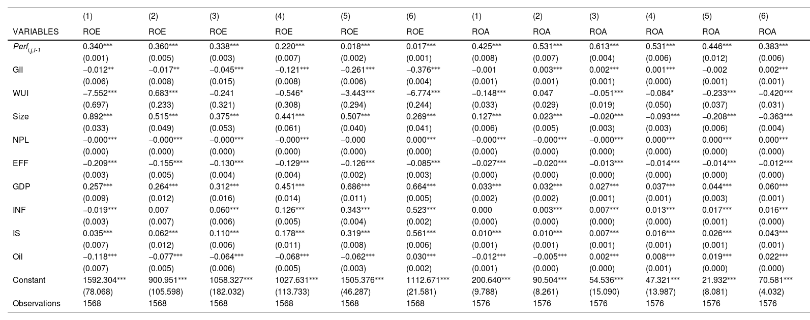
Table 3 gives the descriptive statistics of the variables. The mean of the performance measures can be positive or negative. The means of ROA and Tobin’s Q are positive, showing that these banks perform well. But the opposite is true of ROE and bank stock returns, both of which are negative. This occurs because the method for calculating each variable is different. The GII has a positive mean of 31.82, almost as high as the global level in 2022, 32.09. The three measures of uncertainty are positive and indicate a positive level of uncertainty. For example, thea averages for EPU and GPR are moderate, whereas that of WUI is low.
Descriptive statistics.
Table 4 lists the correlation coefficients of the variables, showing that the relationship of GII to ROA is negative and with Tobin’s Q is positive.EPU and WUI are negatively and significantly associated with ROA and Tobin’s Q. However, GPR appears to have a negative and significant relation to ROA, but it also has a positive and significant link with bank stock returns.
Correlation.
| Variables | (1) | (2) | (3) | (4) | (5) | (6) | (7) | (8) | (9) | (10) | (11) | (12) | (13) | (14) |
|---|---|---|---|---|---|---|---|---|---|---|---|---|---|---|
| (1) ROA | 1 | |||||||||||||
| (2) ROE | 0.046⁎⁎⁎ | 1 | ||||||||||||
| (3) Tobin’s Q | 0.037 | −0.002 | 1 | |||||||||||
| (4) R | −0.113⁎⁎⁎ | −0.009 | 0.106⁎⁎⁎ | 1 | ||||||||||
| (5) GII | −0.043⁎⁎ | 0.003 | 0.093⁎⁎⁎ | −0.026 | 1 | |||||||||
| (6) EPU | −0.036⁎⁎ | 0.002 | −0.047⁎⁎ | −0.036 | −0.147⁎⁎⁎ | 1 | ||||||||
| (7) WUI | −0.046⁎⁎⁎ | −0.006 | −0.069⁎⁎⁎ | −0.005 | −0.017 | 0.034⁎⁎ | 1 | |||||||
| (8) GPR | −0.030* | −0.01 | −0.016 | 0.154⁎⁎⁎ | −0.127⁎⁎⁎ | 0.230⁎⁎⁎ | −0.02 | 1 | ||||||
| (9) Size | −0.053⁎⁎⁎ | 0.021 | −0.143⁎⁎⁎ | 0.019 | 0.338⁎⁎⁎ | 0.067⁎⁎⁎ | −0.039⁎⁎ | 0.018 | 1 | |||||
| (10) NPL | −0.031* | 0.002 | −0.061⁎⁎ | −0.015 | 0.162⁎⁎⁎ | 0.122⁎⁎⁎ | −0.026 | 0.006 | 0.528⁎⁎⁎ | 1 | ||||
| (11) EFF | −0.324⁎⁎⁎ | −0.035⁎⁎ | 0.058⁎⁎ | 0.03 | −0.003 | 0.026 | 0.027 | 0.01 | −0.194⁎⁎⁎ | −0.102⁎⁎⁎ | 1 | |||
| (12) GDP | 0.008 | −0.008 | 0.045* | 0.031 | 0.128⁎⁎⁎ | −0.102⁎⁎⁎ | −0.043⁎⁎⁎ | 0.129⁎⁎⁎ | 0.136⁎⁎⁎ | 0.089⁎⁎⁎ | −0.030* | 1 | ||
| (13) INF | 0.031* | 0.006 | −0.026 | −0.038 | −0.178⁎⁎⁎ | 0.166⁎⁎⁎ | 0.081⁎⁎⁎ | −0.011 | −0.035⁎⁎ | −0.011 | 0.062⁎⁎⁎ | −0.091⁎⁎⁎ | 1 | |
| (14) Oil | 0.002 | 0.017 | 0.143⁎⁎⁎ | 0.033 | 0.053⁎⁎⁎ | −0.162⁎⁎⁎ | −0.183⁎⁎⁎ | −0.089⁎⁎⁎ | −0.004 | 0.098⁎⁎⁎ | 0.030* | 0.160⁎⁎⁎ | −0.050⁎⁎⁎ | 1 |
Tables 5–10 show the results of the QR of the four measures of bank performance with the innovation index and the three measures of uncertainty. The results indicate that the innovation index negatively influences most quantiles’ ROE and bank stock returns. One way of explaining this negative link between GII and ROE is that although innovation might contribute to profitability, it might also increase equity, dilute earnings, and reduce ROE (O’Brien, 2003). Access to capital and a well-developed financial infrastructure are essential for an effective innovation system. Innovation’s positive impact might offset profits due to the simultaneous increase in equity. In addition, the perceived risk associated with a young or early-stage company might make it more difficult to access funds. This has a negative impact on ROE because it results in a larger numerator, which leads to a lower ratio. This supports the resource-based view, which states that a firm’s capabilities and resources create its primary competitive advantage. Companies with unique and valuable resources were more likely to innovate. However, the likelihood of innovation is lower at firms with resources that are imitable and substitutable. Companies with unique and valuable resources are more likely to innovate in order to protect their competitive advantage (Albaity, Saadaoui Mallek, Al-Tamimi, & Molyneux, 2023).
The results of the baseline model of the effect of the uncertainty index EPU and Innovation GII on the bank performance proxies (ROE and ROA).
| (1) | (2) | (3) | (4) | (5) | (6) | (1) | (2) | (3) | (4) | (5) | (6) | |
|---|---|---|---|---|---|---|---|---|---|---|---|---|
| VARIABLES | ROE | ROE | ROE | ROE | ROE | ROE | ROA | ROA | ROA | ROA | ROA | ROA |
| Perfi,j,t-1 | 0.324⁎⁎⁎ | 0.387⁎⁎⁎ | 0.345⁎⁎⁎ | 0.205⁎⁎⁎ | 0.017⁎⁎⁎ | 0.011⁎⁎⁎ | 0.434⁎⁎⁎ | 0.539⁎⁎⁎ | 0.606⁎⁎⁎ | 0.537⁎⁎⁎ | 0.460⁎⁎⁎ | 0.409⁎⁎⁎ |
| (0.004) | (0.003) | (0.002) | (0.005) | (0.002) | (0.002) | (0.009) | (0.004) | (0.005) | (0.019) | (0.008) | (0.006) | |
| GII | −0.040⁎⁎ | −0.017 | −0.035⁎⁎⁎ | −0.079⁎⁎⁎ | −0.235⁎⁎⁎ | −0.353⁎⁎⁎ | −0.003⁎⁎⁎ | 0.005⁎⁎⁎ | 0.003⁎⁎⁎ | 0.005⁎⁎⁎ | 0.006⁎⁎ | 0.012⁎⁎⁎ |
| (0.019) | (0.018) | (0.009) | (0.007) | (0.010) | (0.019) | (0.001) | (0.001) | (0.001) | (0.001) | (0.002) | (0.001) | |
| EPU | −0.043⁎⁎⁎ | −0.032⁎⁎⁎ | −0.013⁎⁎⁎ | −0.000 | 0.006⁎⁎⁎ | −0.013⁎⁎⁎ | −0.004⁎⁎⁎ | −0.004⁎⁎⁎ | −0.002⁎⁎⁎ | −0.003⁎⁎ | −0.000 | −0.000⁎⁎ |
| (0.005) | (0.011) | (0.001) | (0.003) | (0.001) | (0.002) | (0.000) | (0.001) | (0.000) | (0.001) | (0.000) | (0.000) | |
| Size | 1.060⁎⁎⁎ | 0.528⁎⁎⁎ | 0.260⁎⁎⁎ | −0.084⁎⁎⁎ | −0.384⁎⁎⁎ | −0.323⁎⁎⁎ | 0.150⁎⁎⁎ | 0.022⁎⁎⁎ | −0.041⁎⁎⁎ | −0.154⁎⁎⁎ | −0.338⁎⁎⁎ | −0.563⁎⁎⁎ |
| (0.076) | (0.055) | (0.037) | (0.023) | (0.045) | (0.050) | (0.005) | (0.008) | (0.004) | (0.009) | (0.012) | (0.010) | |
| NPL | −0.000⁎⁎⁎ | −0.000⁎⁎⁎ | −0.000⁎⁎⁎ | −0.000⁎⁎⁎ | 0.000⁎⁎⁎ | 0.000⁎⁎⁎ | −0.000⁎⁎⁎ | −0.000⁎⁎⁎ | 0.000 | 0.000⁎⁎⁎ | 0.000⁎⁎⁎ | 0.000⁎⁎⁎ |
| (0.000) | (0.000) | (0.000) | (0.000) | (0.000) | (0.000) | (0.000) | (0.000) | (0.000) | (0.000) | (0.000) | (0.000) | |
| EFF | −0.227⁎⁎⁎ | −0.159⁎⁎⁎ | −0.136⁎⁎⁎ | −0.154⁎⁎⁎ | −0.154⁎⁎⁎ | −0.109⁎⁎⁎ | −0.032⁎⁎⁎ | −0.020⁎⁎⁎ | −0.015⁎⁎⁎ | −0.015⁎⁎⁎ | −0.015⁎⁎⁎ | −0.013⁎⁎⁎ |
| (0.006) | (0.003) | (0.002) | (0.003) | (0.003) | (0.002) | (0.000) | (0.001) | (0.000) | (0.001) | (0.000) | (0.000) | |
| GDP | 0.216⁎⁎⁎ | 0.182⁎⁎⁎ | 0.282⁎⁎⁎ | 0.398⁎⁎⁎ | 0.599⁎⁎⁎ | 0.485⁎⁎⁎ | 0.025⁎⁎⁎ | 0.020⁎⁎⁎ | 0.025⁎⁎⁎ | 0.026⁎⁎⁎ | 0.049⁎⁎⁎ | 0.054⁎⁎⁎ |
| (0.025) | (0.022) | (0.012) | (0.017) | (0.020) | (0.023) | (0.001) | (0.003) | (0.002) | (0.005) | (0.004) | (0.001) | |
| INF | −0.034⁎⁎⁎ | −0.004 | 0.061⁎⁎⁎ | 0.155⁎⁎⁎ | 0.406⁎⁎⁎ | 0.552⁎⁎⁎ | 0.000 | 0.003⁎⁎⁎ | 0.007⁎⁎⁎ | 0.015⁎⁎⁎ | 0.021⁎⁎⁎ | 0.023⁎⁎⁎ |
| (0.007) | (0.008) | (0.003) | (0.004) | (0.005) | (0.006) | (0.000) | (0.001) | (0.000) | (0.001) | (0.000) | (0.000) | |
| IS | 0.047⁎⁎⁎ | 0.049⁎⁎⁎ | 0.094⁎⁎⁎ | 0.156⁎⁎⁎ | 0.223⁎⁎⁎ | 0.398⁎⁎⁎ | 0.009⁎⁎⁎ | 0.007⁎⁎⁎ | 0.006⁎⁎⁎ | 0.013⁎⁎⁎ | 0.026⁎⁎⁎ | 0.024⁎⁎⁎ |
| (0.017) | (0.011) | (0.004) | (0.013) | (0.012) | (0.019) | (0.000) | (0.001) | (0.001) | (0.001) | (0.001) | (0.001) | |
| Oil | −0.138⁎⁎⁎ | −0.081⁎⁎⁎ | −0.062⁎⁎⁎ | −0.058⁎⁎⁎ | −0.004 | 0.071⁎⁎⁎ | −0.011⁎⁎⁎ | −0.004⁎⁎⁎ | 0.001⁎⁎ | 0.009⁎⁎⁎ | 0.018⁎⁎⁎ | 0.029⁎⁎⁎ |
| (0.006) | (0.005) | (0.003) | (0.004) | (0.006) | (0.009) | (0.000) | (0.000) | (0.001) | (0.001) | (0.001) | (0.001) | |
| Constant | −240.373 | −555.216 | 337.766⁎⁎⁎ | 1103.544⁎⁎⁎ | 1862.586⁎⁎⁎ | 341.029⁎⁎⁎ | 13.501* | −77.926* | −34.107⁎⁎ | −84.693 | 82.300⁎⁎⁎ | 57.216⁎⁎⁎ |
| (277.503) | (583.121) | (74.362) | (159.182) | (83.805) | (110.347) | (7.927) | (40.614) | (15.132) | (61.490) | (21.550) | (16.818) | |
| Observations | 1763 | 1763 | 1763 | 1763 | 1763 | 1763 | 1771 | 1771 | 1771 | 1771 | 1771 | 1771 |
Notes: Perfi,j,t-1, the lagged value of the bank performance proxies namely (ROE and ROA); GII, the Global Innovation Index; EPU the Economic Policy Uncertainty index; Size is the bank size, NPl is the non-performing loans ratio; EFF is the efficiency cost-to-income ratio; GDP is the gross domestic product; INF is the inflation level proxied by the consumer price index; is a dummy for the bank type which equates 1 if the bank is Islamic and zero otherwise; and Oil, oil price.
Note: Standard errors in parentheses;.
The results of the baseline model of the effect of the uncertainty index EPU and Innovation GII on the bank performance proxies (R and Tobin’s).
| (1) | (2) | (3) | (4) | (5) | (6) | (1) | (2) | (3) | (4) | (5) | (6) | |
|---|---|---|---|---|---|---|---|---|---|---|---|---|
| VARIABLES | R | R | R | R | R | R | Tobin’s Q | Tobin’s Q | Tobin’s Q | Tobin’s Q | Tobin’s Q | Tobin’s Q |
| Perfi,j,t-1 | −0.070⁎⁎⁎ | −0.068⁎⁎⁎ | −0.038⁎⁎ | −0.037⁎⁎⁎ | 0.045⁎⁎⁎ | 0.049⁎⁎⁎ | 0.656⁎⁎⁎ | 0.768⁎⁎⁎ | 0.904⁎⁎⁎ | 0.997⁎⁎⁎ | 1.028⁎⁎⁎ | 0.983⁎⁎⁎ |
| (0.012) | (0.008) | (0.015) | (0.014) | (0.017) | (0.014) | (0.003) | (0.003) | (0.004) | (0.005) | (0.003) | (0.002) | |
| GII | 0.001⁎⁎⁎ | −0.003⁎⁎⁎ | −0.002⁎⁎⁎ | −0.001 | 0.000 | −0.001⁎⁎⁎ | 0.000⁎⁎⁎ | 0.000⁎⁎⁎ | 0.000⁎⁎⁎ | 0.000⁎⁎⁎ | 0.001⁎⁎⁎ | 0.000⁎⁎⁎ |
| (0.000) | (0.000) | (0.001) | (0.001) | (0.001) | (0.000) | (0.000) | (0.000) | (0.000) | (0.000) | (0.000) | (0.000) | |
| EPU | −0.002⁎⁎⁎ | −0.001⁎⁎⁎ | −0.001⁎⁎⁎ | −0.001⁎⁎⁎ | −0.002⁎⁎⁎ | −0.002⁎⁎⁎ | −0.000⁎⁎⁎ | −0.000⁎⁎⁎ | −0.000* | −0.000 | 0.000 | 0.000⁎⁎⁎ |
| (0.000) | (0.000) | (0.000) | (0.000) | (0.000) | (0.000) | (0.000) | (0.000) | (0.000) | (0.000) | (0.000) | (0.000) | |
| Size | −0.011⁎⁎⁎ | −0.002 | −0.009⁎⁎⁎ | −0.019⁎⁎⁎ | −0.021⁎⁎⁎ | −0.031⁎⁎⁎ | −0.001⁎⁎⁎ | −0.000 | −0.001⁎⁎⁎ | −0.004⁎⁎⁎ | −0.006⁎⁎⁎ | −0.009⁎⁎⁎ |
| (0.003) | (0.003) | (0.001) | (0.002) | (0.004) | (0.002) | (0.000) | (0.000) | (0.001) | (0.001) | (0.000) | (0.000) | |
| NPL | −0.000⁎⁎⁎ | −0.000 | 0.000 | 0.000⁎⁎⁎ | 0.000⁎⁎⁎ | 0.000⁎⁎⁎ | 0.000⁎⁎⁎ | 0.000⁎⁎⁎ | 0.000⁎⁎⁎ | 0.000⁎⁎⁎ | 0.000⁎⁎⁎ | 0.000⁎⁎⁎ |
| (0.000) | (0.000) | (0.000) | (0.000) | (0.000) | (0.000) | (0.000) | (0.000) | (0.000) | (0.000) | (0.000) | (0.000) | |
| EFF | −0.001⁎⁎⁎ | 0.000* | 0.000⁎⁎⁎ | 0.001⁎⁎⁎ | 0.004⁎⁎⁎ | 0.005⁎⁎⁎ | −0.000⁎⁎⁎ | −0.000⁎⁎⁎ | −0.000⁎⁎⁎ | −0.000⁎⁎⁎ | −0.000⁎⁎⁎ | −0.000⁎⁎⁎ |
| (0.000) | (0.000) | (0.000) | (0.000) | (0.000) | (0.000) | (0.000) | (0.000) | (0.000) | (0.000) | (0.000) | (0.000) | |
| GDP | −0.005⁎⁎⁎ | 0.001 | 0.001 | 0.006⁎⁎⁎ | 0.007⁎⁎⁎ | 0.010⁎⁎⁎ | −0.000⁎⁎⁎ | −0.000 | 0.001⁎⁎⁎ | 0.001⁎⁎⁎ | 0.002⁎⁎⁎ | 0.004⁎⁎⁎ |
| (0.001) | (0.001) | (0.001) | (0.001) | (0.001) | (0.001) | (0.000) | (0.000) | (0.000) | (0.000) | (0.000) | (0.000) | |
| INF | −0.006⁎⁎⁎ | −0.003⁎⁎⁎ | −0.001⁎⁎⁎ | 0.000⁎⁎ | 0.003⁎⁎⁎ | 0.003⁎⁎⁎ | 0.000* | 0.000⁎⁎⁎ | 0.000⁎⁎⁎ | 0.001⁎⁎⁎ | 0.001⁎⁎⁎ | 0.001⁎⁎⁎ |
| (0.000) | (0.000) | (0.000) | (0.000) | (0.000) | (0.000) | (0.000) | (0.000) | (0.000) | (0.000) | (0.000) | (0.000) | |
| IS | −0.004⁎⁎⁎ | −0.003⁎⁎⁎ | −0.002⁎⁎⁎ | −0.003⁎⁎⁎ | −0.001⁎⁎⁎ | −0.004⁎⁎⁎ | −0.000⁎⁎⁎ | −0.000 | −0.000 | 0.000⁎⁎⁎ | 0.001⁎⁎⁎ | 0.001⁎⁎⁎ |
| (0.001) | (0.000) | (0.000) | (0.000) | (0.001) | (0.000) | (0.000) | (0.000) | (0.000) | (0.000) | (0.000) | (0.000) | |
| Oil | 0.000 | −0.000 | 0.001⁎⁎⁎ | 0.004⁎⁎⁎ | 0.005⁎⁎⁎ | 0.007⁎⁎⁎ | 0.000⁎⁎⁎ | 0.000⁎⁎⁎ | 0.000⁎⁎⁎ | 0.000⁎⁎⁎ | 0.001⁎⁎⁎ | 0.001⁎⁎⁎ |
| (0.000) | (0.000) | (0.000) | (0.000) | (0.000) | (0.000) | (0.000) | (0.000) | (0.000) | (0.000) | (0.000) | (0.000) | |
| Constant | −73.910⁎⁎⁎ | −23.119 | −23.362* | −28.344⁎⁎⁎ | −86.993⁎⁎⁎ | −140.649⁎⁎⁎ | −3.039⁎⁎⁎ | −2.859⁎⁎ | −1.339 | 1.042 | 2.640⁎⁎⁎ | 6.798⁎⁎⁎ |
| (7.134) | (16.935) | (13.220) | (9.659) | (3.095) | (2.567) | (0.544) | (1.331) | (1.415) | (1.525) | (0.969) | (0.760) | |
| Observations | 951 | 951 | 951 | 951 | 951 | 951 | 934 | 934 | 934 | 934 | 934 | 934 |
Notes: variables defined same as in Table 5 except two dependent variables proxies (R and Tobin’s).
Note: Standard errors in parentheses;.
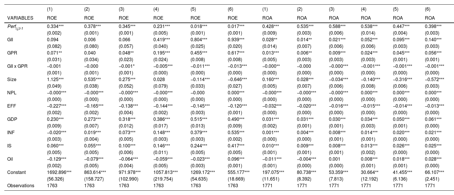
The results of the baseline model of the effect of the uncertainty index GPR and Innovation GII on the bank performance proxies (ROE and ROA).
| (1) | (2) | (3) | (4) | (5) | (6) | (1) | (2) | (3) | (4) | (5) | (6) | |
|---|---|---|---|---|---|---|---|---|---|---|---|---|
| VARIABLES | ROE | ROE | ROE | ROE | ROE | ROE | ROA | ROA | ROA | ROA | ROA | ROA |
| Perfi,j,t-1 | 0.338⁎⁎⁎ | 0.378⁎⁎⁎ | 0.340⁎⁎⁎ | 0.221⁎⁎⁎ | 0.020⁎⁎⁎ | 0.017⁎⁎⁎ | 0.428⁎⁎⁎ | 0.547⁎⁎⁎ | 0.591⁎⁎⁎ | 0.536⁎⁎⁎ | 0.452⁎⁎⁎ | 0.400⁎⁎⁎ |
| (0.002) | (0.002) | (0.004) | (0.008) | (0.003) | (0.001) | (0.007) | (0.010) | (0.004) | (0.014) | (0.008) | (0.003) | |
| GII | −0.044⁎⁎⁎ | −0.030⁎⁎⁎ | −0.031 | −0.082⁎⁎⁎ | −0.236⁎⁎⁎ | −0.253⁎⁎⁎ | −0.004⁎⁎⁎ | 0.003⁎⁎⁎ | 0.003⁎⁎⁎ | 0.003⁎⁎⁎ | 0.005⁎⁎⁎ | 0.013⁎⁎⁎ |
| (0.009) | (0.007) | (0.019) | (0.009) | (0.006) | (0.002) | (0.001) | (0.001) | (0.001) | (0.001) | (0.002) | (0.001) | |
| GPR | 0.026⁎⁎⁎ | 0.015 | 0.013 | 0.012* | 0.072⁎⁎⁎ | 0.145⁎⁎⁎ | 0.003⁎⁎⁎ | 0.002⁎⁎⁎ | 0.002⁎⁎⁎ | 0.005⁎⁎⁎ | 0.005⁎⁎⁎ | 0.005⁎⁎⁎ |
| (0.006) | (0.010) | (0.008) | (0.007) | (0.006) | (0.003) | (0.001) | (0.001) | (0.000) | (0.001) | (0.001) | (0.000) | |
| Size | 1.054⁎⁎⁎ | 0.526⁎⁎⁎ | 0.256⁎⁎⁎ | −0.067* | −0.317⁎⁎⁎ | −0.599⁎⁎⁎ | 0.156⁎⁎⁎ | 0.025⁎⁎⁎ | −0.041⁎⁎⁎ | −0.138⁎⁎⁎ | −0.331⁎⁎⁎ | −0.581⁎⁎⁎ |
| (0.038) | (0.046) | (0.064) | (0.040) | (0.035) | (0.050) | (0.009) | (0.007) | (0.004) | (0.007) | (0.014) | (0.003) | |
| NPL | −0.000⁎⁎⁎ | −0.000⁎⁎⁎ | −0.000⁎⁎⁎ | −0.000⁎⁎⁎ | 0.000 | 0.000⁎⁎⁎ | −0.000⁎⁎⁎ | −0.000⁎⁎⁎ | −0.000 | 0.000⁎⁎⁎ | 0.000⁎⁎⁎ | 0.000⁎⁎⁎ |
| (0.000) | (0.000) | (0.000) | (0.000) | (0.000) | (0.000) | (0.000) | (0.000) | (0.000) | (0.000) | (0.000) | (0.000) | |
| EFF | −0.225⁎⁎⁎ | −0.165⁎⁎⁎ | −0.135⁎⁎⁎ | −0.148⁎⁎⁎ | −0.149⁎⁎⁎ | −0.121⁎⁎⁎ | −0.032⁎⁎⁎ | −0.020⁎⁎⁎ | −0.016⁎⁎⁎ | −0.015⁎⁎⁎ | −0.015⁎⁎⁎ | −0.013⁎⁎⁎ |
| (0.004) | (0.002) | (0.003) | (0.004) | (0.005) | (0.001) | (0.000) | (0.000) | (0.000) | (0.000) | (0.000) | (0.000) | |
| GDP | 0.257⁎⁎⁎ | 0.267⁎⁎⁎ | 0.313⁎⁎⁎ | 0.378⁎⁎⁎ | 0.490⁎⁎⁎ | 0.464⁎⁎⁎ | 0.034⁎⁎⁎ | 0.031⁎⁎⁎ | 0.029⁎⁎⁎ | 0.035⁎⁎⁎ | 0.048⁎⁎⁎ | 0.053⁎⁎⁎ |
| (0.010) | (0.013) | (0.013) | (0.017) | (0.025) | (0.005) | (0.002) | (0.002) | (0.001) | (0.001) | (0.002) | (0.001) | |
| INF | −0.018⁎⁎⁎ | 0.022⁎⁎⁎ | 0.068⁎⁎⁎ | 0.155⁎⁎⁎ | 0.420⁎⁎⁎ | 0.582⁎⁎⁎ | 0.001⁎⁎⁎ | 0.004⁎⁎⁎ | 0.008⁎⁎⁎ | 0.014⁎⁎⁎ | 0.021⁎⁎⁎ | 0.023⁎⁎⁎ |
| (0.005) | (0.004) | (0.006) | (0.005) | (0.006) | (0.003) | (0.000) | (0.001) | (0.000) | (0.001) | (0.000) | (0.000) | |
| IS | 0.055⁎⁎⁎ | 0.062⁎⁎⁎ | 0.091⁎⁎⁎ | 0.155⁎⁎⁎ | 0.213⁎⁎⁎ | 0.388⁎⁎⁎ | 0.011⁎⁎⁎ | 0.009⁎⁎⁎ | 0.008⁎⁎⁎ | 0.013⁎⁎⁎ | 0.027⁎⁎⁎ | 0.025⁎⁎⁎ |
| (0.011) | (0.008) | (0.009) | (0.006) | (0.011) | (0.006) | (0.002) | (0.001) | (0.001) | (0.001) | (0.001) | (0.000) | |
| Oil | −0.121⁎⁎⁎ | −0.081⁎⁎⁎ | −0.059⁎⁎⁎ | −0.054⁎⁎⁎ | 0.001 | 0.128⁎⁎⁎ | −0.011⁎⁎⁎ | −0.005⁎⁎⁎ | 0.001⁎⁎⁎ | 0.009⁎⁎⁎ | 0.017⁎⁎⁎ | 0.029⁎⁎⁎ |
| (0.007) | (0.004) | (0.005) | (0.004) | (0.005) | (0.002) | (0.001) | (0.001) | (0.000) | (0.001) | (0.001) | (0.000) | |
| Constant | 1690.481⁎⁎⁎ | 1081.911⁎⁎⁎ | 844.613⁎⁎⁎ | 1040.535⁎⁎⁎ | 1040.355⁎⁎⁎ | 264.516⁎⁎⁎ | 219.342⁎⁎⁎ | 84.638⁎⁎⁎ | 49.244⁎⁎⁎ | 34.096⁎⁎⁎ | 58.080⁎⁎⁎ | 14.982⁎⁎⁎ |
| (55.088) | (136.930) | (235.270) | (100.704) | (37.038) | (12.614) | (5.653) | (18.037) | (6.917) | (8.278) | (14.243) | (3.977) | |
| Observations | 1763 | 1763 | 1763 | 1763 | 1763 | 1763 | 1771 | 1771 | 1771 | 1771 | 1771 | 1771 |
Notes: variables defined same as in Table 5 except for the uncertainty index namely the Geopolitical Risk GPR.
Standard errors in parentheses;.
The results of the baseline model of the effect of the uncertainty index GPR and Innovation GII on the bank performance proxies (R and Tobin’s).
| (1) | (2) | (3) | (4) | (5) | (6) | (1) | (2) | (3) | (4) | (5) | (6) | |
|---|---|---|---|---|---|---|---|---|---|---|---|---|
| VARIABLES | R | R | R | R | R | R | Tobin’s Q | Tobin’s Q | Tobin’s Q | Tobin’s Q | Tobin’s Q | Tobin’s Q |
| Perfi,j,t-1 | −0.129⁎⁎⁎ | −0.078⁎⁎⁎ | −0.065⁎⁎⁎ | −0.079⁎⁎⁎ | −0.001 | 0.108⁎⁎⁎ | 0.654⁎⁎⁎ | 0.773⁎⁎⁎ | 0.907⁎⁎⁎ | 1.002⁎⁎⁎ | 1.036⁎⁎⁎ | 1.030⁎⁎⁎ |
| (0.008) | (0.007) | (0.014) | (0.020) | (0.014) | (0.022) | (0.001) | (0.004) | (0.005) | (0.007) | (0.006) | (0.001) | |
| GII | 0.002⁎⁎⁎ | −0.002⁎⁎⁎ | −0.000 | 0.000 | −0.001 | −0.002⁎⁎ | 0.000⁎⁎⁎ | 0.000⁎⁎⁎ | 0.000⁎⁎⁎ | 0.000⁎⁎⁎ | 0.001⁎⁎⁎ | 0.000⁎⁎⁎ |
| (0.000) | (0.001) | (0.000) | (0.001) | (0.001) | (0.001) | (0.000) | (0.000) | (0.000) | (0.000) | (0.000) | (0.000) | |
| GPR | 0.005⁎⁎⁎ | 0.004⁎⁎⁎ | 0.005⁎⁎⁎ | 0.006⁎⁎⁎ | 0.007⁎⁎⁎ | 0.012⁎⁎⁎ | −0.000⁎⁎⁎ | −0.000 | −0.000⁎⁎⁎ | −0.001⁎⁎⁎ | −0.001⁎⁎⁎ | −0.001⁎⁎⁎ |
| (0.000) | (0.000) | (0.001) | (0.000) | (0.001) | (0.000) | (0.000) | (0.000) | (0.000) | (0.000) | (0.000) | (0.000) | |
| Size | −0.022⁎⁎⁎ | −0.010⁎⁎ | −0.017⁎⁎⁎ | −0.017⁎⁎⁎ | −0.021⁎⁎⁎ | −0.023⁎⁎⁎ | −0.001⁎⁎⁎ | −0.001⁎⁎ | −0.001⁎⁎⁎ | −0.003⁎⁎⁎ | −0.006⁎⁎⁎ | −0.008⁎⁎⁎ |
| (0.001) | (0.004) | (0.004) | (0.002) | (0.005) | (0.006) | (0.000) | (0.000) | (0.000) | (0.001) | (0.001) | (0.000) | |
| NPL | −0.000⁎⁎⁎ | −0.000 | 0.000 | 0.000⁎⁎⁎ | 0.000⁎⁎⁎ | 0.000 | 0.000⁎⁎⁎ | 0.000⁎⁎⁎ | 0.000⁎⁎⁎ | 0.000⁎⁎⁎ | 0.000⁎⁎⁎ | 0.000⁎⁎⁎ |
| (0.000) | (0.000) | (0.000) | (0.000) | (0.000) | (0.000) | (0.000) | (0.000) | (0.000) | (0.000) | (0.000) | (0.000) | |
| EFF | −0.001⁎⁎⁎ | 0.000 | 0.001⁎⁎⁎ | 0.002⁎⁎⁎ | 0.004⁎⁎⁎ | 0.006⁎⁎⁎ | −0.000⁎⁎⁎ | −0.000⁎⁎⁎ | −0.000⁎⁎⁎ | −0.000⁎⁎⁎ | −0.000⁎⁎⁎ | −0.000⁎⁎⁎ |
| (0.000) | (0.000) | (0.000) | (0.000) | (0.000) | (0.000) | (0.000) | (0.000) | (0.000) | (0.000) | (0.000) | (0.000) | |
| GDP | 0.001⁎⁎ | 0.003⁎⁎⁎ | 0.000 | 0.004⁎⁎⁎ | 0.008⁎⁎⁎ | 0.009⁎⁎⁎ | 0.000⁎⁎⁎ | 0.000⁎⁎⁎ | 0.001⁎⁎⁎ | 0.002⁎⁎⁎ | 0.002⁎⁎⁎ | 0.003⁎⁎⁎ |
| (0.000) | (0.001) | (0.001) | (0.001) | (0.001) | (0.001) | (0.000) | (0.000) | (0.000) | (0.000) | (0.000) | (0.000) | |
| INF | −0.004⁎⁎⁎ | −0.002⁎⁎⁎ | −0.001⁎⁎⁎ | 0.001⁎⁎⁎ | 0.004⁎⁎⁎ | 0.008⁎⁎⁎ | 0.000⁎⁎⁎ | 0.000⁎⁎⁎ | 0.001⁎⁎⁎ | 0.001⁎⁎⁎ | 0.001⁎⁎⁎ | 0.001⁎⁎⁎ |
| (0.000) | (0.000) | (0.000) | (0.000) | (0.001) | (0.000) | (0.000) | (0.000) | (0.000) | (0.000) | (0.000) | (0.000) | |
| IS | −0.004⁎⁎⁎ | −0.004⁎⁎⁎ | −0.002⁎⁎⁎ | −0.003⁎⁎⁎ | −0.002⁎⁎⁎ | −0.002⁎⁎⁎ | −0.000⁎⁎⁎ | −0.000 | −0.000 | 0.000⁎⁎⁎ | 0.001⁎⁎⁎ | 0.001⁎⁎⁎ |
| (0.000) | (0.000) | (0.000) | (0.001) | (0.001) | (0.000) | (0.000) | (0.000) | (0.000) | (0.000) | (0.000) | (0.000) | |
| Oil | 0.001⁎⁎⁎ | 0.000⁎⁎ | 0.002⁎⁎⁎ | 0.004⁎⁎⁎ | 0.005⁎⁎⁎ | 0.009⁎⁎⁎ | 0.000⁎⁎⁎ | 0.000⁎⁎⁎ | 0.000⁎⁎⁎ | 0.000⁎⁎⁎ | 0.001⁎⁎⁎ | 0.001⁎⁎⁎ |
| (0.000) | (0.000) | (0.000) | (0.000) | (0.000) | (0.000) | (0.000) | (0.000) | (0.000) | (0.000) | (0.000) | (0.000) | |
| Constant | −10.223⁎⁎⁎ | −1.094 | −13.718 | −20.816⁎⁎⁎ | −18.679⁎⁎⁎ | −37.494⁎⁎⁎ | 0.729⁎⁎⁎ | −0.629 | 2.933⁎⁎ | 5.362⁎⁎⁎ | 2.460⁎⁎⁎ | 6.872⁎⁎⁎ |
| (2.782) | (7.267) | (8.942) | (4.213) | (6.849) | (4.842) | (0.122) | (1.144) | (1.253) | (1.133) | (0.515) | (0.202) | |
| Observations | 951 | 951 | 951 | 951 | 951 | 951 | 934 | 934 | 934 | 934 | 934 | 934 |
Notes: variables defined same as in Table 6 except for the uncertainty index namely the Geopolitical Risk GPR.
Standard errors in parentheses;.
The results of the baseline model of the effect of the uncertainty index WUI and Innovation GII on the bank performance proxies (ROE and ROA).
| (1) | (2) | (3) | (4) | (5) | (6) | (1) | (2) | (3) | (4) | (5) | (6) | |
|---|---|---|---|---|---|---|---|---|---|---|---|---|
| VARIABLES | ROE | ROE | ROE | ROE | ROE | ROE | ROA | ROA | ROA | ROA | ROA | ROA |
| Perfi,j,t-1 | 0.340⁎⁎⁎ | 0.360⁎⁎⁎ | 0.338⁎⁎⁎ | 0.220⁎⁎⁎ | 0.018⁎⁎⁎ | 0.017⁎⁎⁎ | 0.425⁎⁎⁎ | 0.531⁎⁎⁎ | 0.613⁎⁎⁎ | 0.531⁎⁎⁎ | 0.446⁎⁎⁎ | 0.383⁎⁎⁎ |
| (0.001) | (0.005) | (0.003) | (0.007) | (0.002) | (0.001) | (0.008) | (0.007) | (0.004) | (0.006) | (0.012) | (0.006) | |
| GII | −0.012⁎⁎ | −0.017⁎⁎ | −0.045⁎⁎⁎ | −0.121⁎⁎⁎ | −0.261⁎⁎⁎ | −0.376⁎⁎⁎ | −0.001 | 0.003⁎⁎⁎ | 0.002⁎⁎⁎ | 0.001⁎⁎⁎ | −0.002 | 0.002⁎⁎⁎ |
| (0.006) | (0.008) | (0.015) | (0.008) | (0.006) | (0.004) | (0.001) | (0.001) | (0.001) | (0.000) | (0.001) | (0.001) | |
| WUI | −7.552⁎⁎⁎ | 0.683⁎⁎⁎ | −0.241 | −0.546* | −3.443⁎⁎⁎ | −6.774⁎⁎⁎ | −0.148⁎⁎⁎ | 0.047 | −0.051⁎⁎⁎ | −0.084* | −0.233⁎⁎⁎ | −0.420⁎⁎⁎ |
| (0.697) | (0.233) | (0.321) | (0.308) | (0.294) | (0.244) | (0.033) | (0.029) | (0.019) | (0.050) | (0.037) | (0.031) | |
| Size | 0.892⁎⁎⁎ | 0.515⁎⁎⁎ | 0.375⁎⁎⁎ | 0.441⁎⁎⁎ | 0.507⁎⁎⁎ | 0.269⁎⁎⁎ | 0.127⁎⁎⁎ | 0.023⁎⁎⁎ | −0.020⁎⁎⁎ | −0.093⁎⁎⁎ | −0.208⁎⁎⁎ | −0.363⁎⁎⁎ |
| (0.033) | (0.049) | (0.053) | (0.061) | (0.040) | (0.041) | (0.006) | (0.005) | (0.003) | (0.003) | (0.006) | (0.004) | |
| NPL | −0.000⁎⁎⁎ | −0.000⁎⁎⁎ | −0.000⁎⁎⁎ | −0.000⁎⁎⁎ | −0.000 | 0.000⁎⁎⁎ | −0.000⁎⁎⁎ | −0.000⁎⁎⁎ | −0.000⁎⁎⁎ | 0.000⁎⁎⁎ | 0.000⁎⁎⁎ | 0.000⁎⁎⁎ |
| (0.000) | (0.000) | (0.000) | (0.000) | (0.000) | (0.000) | (0.000) | (0.000) | (0.000) | (0.000) | (0.000) | (0.000) | |
| EFF | −0.209⁎⁎⁎ | −0.155⁎⁎⁎ | −0.130⁎⁎⁎ | −0.129⁎⁎⁎ | −0.126⁎⁎⁎ | −0.085⁎⁎⁎ | −0.027⁎⁎⁎ | −0.020⁎⁎⁎ | −0.013⁎⁎⁎ | −0.014⁎⁎⁎ | −0.014⁎⁎⁎ | −0.012⁎⁎⁎ |
| (0.003) | (0.005) | (0.004) | (0.004) | (0.002) | (0.003) | (0.000) | (0.000) | (0.000) | (0.000) | (0.000) | (0.000) | |
| GDP | 0.257⁎⁎⁎ | 0.264⁎⁎⁎ | 0.312⁎⁎⁎ | 0.451⁎⁎⁎ | 0.686⁎⁎⁎ | 0.664⁎⁎⁎ | 0.033⁎⁎⁎ | 0.032⁎⁎⁎ | 0.027⁎⁎⁎ | 0.037⁎⁎⁎ | 0.044⁎⁎⁎ | 0.060⁎⁎⁎ |
| (0.009) | (0.012) | (0.016) | (0.014) | (0.011) | (0.005) | (0.002) | (0.002) | (0.001) | (0.001) | (0.003) | (0.001) | |
| INF | −0.019⁎⁎⁎ | 0.007 | 0.060⁎⁎⁎ | 0.126⁎⁎⁎ | 0.343⁎⁎⁎ | 0.523⁎⁎⁎ | 0.000 | 0.003⁎⁎⁎ | 0.007⁎⁎⁎ | 0.013⁎⁎⁎ | 0.017⁎⁎⁎ | 0.016⁎⁎⁎ |
| (0.003) | (0.007) | (0.006) | (0.005) | (0.004) | (0.002) | (0.000) | (0.000) | (0.000) | (0.000) | (0.001) | (0.000) | |
| IS | 0.035⁎⁎⁎ | 0.062⁎⁎⁎ | 0.110⁎⁎⁎ | 0.178⁎⁎⁎ | 0.319⁎⁎⁎ | 0.561⁎⁎⁎ | 0.010⁎⁎⁎ | 0.010⁎⁎⁎ | 0.007⁎⁎⁎ | 0.016⁎⁎⁎ | 0.026⁎⁎⁎ | 0.043⁎⁎⁎ |
| (0.007) | (0.012) | (0.006) | (0.011) | (0.008) | (0.006) | (0.001) | (0.001) | (0.001) | (0.001) | (0.001) | (0.001) | |
| Oil | −0.118⁎⁎⁎ | −0.077⁎⁎⁎ | −0.064⁎⁎⁎ | −0.068⁎⁎⁎ | −0.062⁎⁎⁎ | 0.030⁎⁎⁎ | −0.012⁎⁎⁎ | −0.005⁎⁎⁎ | 0.002⁎⁎⁎ | 0.008⁎⁎⁎ | 0.019⁎⁎⁎ | 0.022⁎⁎⁎ |
| (0.007) | (0.005) | (0.006) | (0.005) | (0.003) | (0.002) | (0.001) | (0.000) | (0.000) | (0.001) | (0.000) | (0.000) | |
| Constant | 1592.304⁎⁎⁎ | 900.951⁎⁎⁎ | 1058.327⁎⁎⁎ | 1027.631⁎⁎⁎ | 1505.376⁎⁎⁎ | 1112.671⁎⁎⁎ | 200.640⁎⁎⁎ | 90.504⁎⁎⁎ | 54.536⁎⁎⁎ | 47.321⁎⁎⁎ | 21.932⁎⁎⁎ | 70.581⁎⁎⁎ |
| (78.068) | (105.598) | (182.032) | (113.733) | (46.287) | (21.581) | (9.788) | (8.261) | (15.090) | (13.987) | (8.081) | (4.032) | |
| Observations | 1568 | 1568 | 1568 | 1568 | 1568 | 1568 | 1576 | 1576 | 1576 | 1576 | 1576 | 1576 |
Notes: variables defined same as in Table 5 except for the uncertainty index namely the World Uncertainty Index WUI.
Standard errors in parentheses;.
The results of the baseline model of the effect of the uncertainty index WUI and Innovation GII on the bank performance proxies (R and Tobin’s).
| (1) | (2) | (3) | (4) | (5) | (6) | (1) | (2) | (3) | (4) | (5) | (6) | |
|---|---|---|---|---|---|---|---|---|---|---|---|---|
| VARIABLES | R | R | R | R | R | R | Tobin’s Q | Tobin’s Q | Tobin’s Q | Tobin’s Q | Tobin’s Q | Tobin’s Q |
| Perfi,j,t-1 | −0.045⁎⁎⁎ | −0.066⁎⁎⁎ | −0.018 | −0.023⁎⁎⁎ | 0.070⁎⁎⁎ | 0.225⁎⁎⁎ | 0.672⁎⁎⁎ | 0.769⁎⁎⁎ | 0.900⁎⁎⁎ | 0.999⁎⁎⁎ | 1.026⁎⁎⁎ | 0.978⁎⁎⁎ |
| (0.002) | (0.010) | (0.013) | (0.008) | (0.009) | (0.006) | (0.003) | (0.003) | (0.006) | (0.005) | (0.006) | (0.003) | |
| GII | 0.000 | −0.002⁎⁎⁎ | −0.002⁎⁎⁎ | −0.001* | −0.000 | −0.004⁎⁎⁎ | 0.000⁎⁎⁎ | 0.000⁎⁎ | 0.000⁎⁎ | 0.000⁎⁎⁎ | 0.000⁎⁎⁎ | 0.001⁎⁎⁎ |
| (0.000) | (0.001) | (0.001) | (0.000) | (0.000) | (0.000) | (0.000) | (0.000) | (0.000) | (0.000) | (0.000) | (0.000) | |
| WUI | −0.348⁎⁎⁎ | −0.134⁎⁎⁎ | −0.094⁎⁎ | −0.041 | 0.224⁎⁎⁎ | −0.090⁎⁎⁎ | −0.004⁎⁎ | −0.012⁎⁎⁎ | −0.009⁎⁎ | −0.005 | −0.007⁎⁎⁎ | −0.021⁎⁎⁎ |
| (0.009) | (0.019) | (0.045) | (0.029) | (0.033) | (0.013) | (0.002) | (0.002) | (0.004) | (0.005) | (0.002) | (0.001) | |
| Size | −0.018⁎⁎⁎ | −0.020⁎⁎⁎ | −0.017⁎⁎⁎ | −0.021⁎⁎⁎ | −0.026⁎⁎⁎ | −0.001 | −0.001⁎⁎⁎ | 0.000 | −0.000 | −0.001⁎⁎ | −0.006⁎⁎⁎ | −0.010⁎⁎⁎ |
| (0.002) | (0.002) | (0.004) | (0.002) | (0.004) | (0.002) | (0.000) | (0.000) | (0.000) | (0.001) | (0.000) | (0.000) | |
| NPL | −0.000⁎⁎ | −0.000 | 0.000 | 0.000⁎⁎⁎ | 0.000⁎⁎⁎ | −0.000 | 0.000⁎⁎⁎ | 0.000⁎⁎⁎ | 0.000⁎⁎⁎ | 0.000⁎⁎⁎ | 0.000⁎⁎⁎ | 0.000⁎⁎⁎ |
| (0.000) | (0.000) | (0.000) | (0.000) | (0.000) | (0.000) | (0.000) | (0.000) | (0.000) | (0.000) | (0.000) | (0.000) | |
| EFF | −0.001⁎⁎⁎ | 0.000 | 0.000⁎⁎ | 0.001⁎⁎⁎ | 0.003⁎⁎⁎ | 0.005⁎⁎⁎ | −0.000⁎⁎⁎ | −0.000⁎⁎⁎ | −0.000⁎⁎⁎ | −0.000⁎⁎⁎ | −0.000⁎⁎⁎ | −0.000⁎⁎⁎ |
| (0.000) | (0.000) | (0.000) | (0.000) | (0.000) | (0.000) | (0.000) | (0.000) | (0.000) | (0.000) | (0.000) | (0.000) | |
| GDP | 0.005⁎⁎⁎ | 0.007⁎⁎⁎ | 0.007⁎⁎⁎ | 0.009⁎⁎⁎ | 0.014⁎⁎⁎ | 0.024⁎⁎⁎ | 0.000 | 0.001⁎⁎⁎ | 0.001⁎⁎⁎ | 0.002⁎⁎⁎ | 0.002⁎⁎⁎ | 0.003⁎⁎⁎ |
| (0.000) | (0.001) | (0.001) | (0.001) | (0.001) | (0.001) | (0.000) | (0.000) | (0.000) | (0.000) | (0.000) | (0.000) | |
| INF | −0.001⁎⁎⁎ | −0.001⁎⁎ | 0.000 | 0.001⁎⁎⁎ | 0.002⁎⁎⁎ | 0.004⁎⁎⁎ | 0.000⁎⁎⁎ | 0.000⁎⁎⁎ | 0.000⁎⁎⁎ | 0.001⁎⁎⁎ | 0.001⁎⁎⁎ | 0.001⁎⁎⁎ |
| (0.000) | (0.000) | (0.001) | (0.000) | (0.000) | (0.000) | (0.000) | (0.000) | (0.000) | (0.000) | (0.000) | (0.000) | |
| IS | −0.005⁎⁎⁎ | −0.004⁎⁎⁎ | −0.003⁎⁎⁎ | −0.004⁎⁎⁎ | −0.002⁎⁎⁎ | −0.004⁎⁎⁎ | −0.000* | 0.000⁎⁎⁎ | 0.000⁎⁎⁎ | 0.000⁎⁎⁎ | 0.001⁎⁎⁎ | 0.002⁎⁎⁎ |
| (0.000) | (0.000) | (0.001) | (0.000) | (0.000) | (0.000) | (0.000) | (0.000) | (0.000) | (0.000) | (0.000) | (0.000) | |
| Oil | −0.000 | 0.001⁎⁎⁎ | 0.002⁎⁎⁎ | 0.004⁎⁎⁎ | 0.005⁎⁎⁎ | 0.006⁎⁎⁎ | 0.000⁎⁎⁎ | 0.000⁎⁎⁎ | 0.000⁎⁎⁎ | 0.000⁎⁎⁎ | 0.001⁎⁎⁎ | 0.001⁎⁎⁎ |
| (0.000) | (0.000) | (0.000) | (0.000) | (0.000) | (0.000) | (0.000) | (0.000) | (0.000) | (0.000) | (0.000) | (0.000) | |
| Constant | 13.825⁎⁎⁎ | 18.290⁎⁎⁎ | 14.218 | 3.006 | 13.327⁎⁎⁎ | 3.615⁎⁎⁎ | 1.014⁎⁎⁎ | 1.796⁎⁎⁎ | 2.610⁎⁎ | 2.100⁎⁎⁎ | −0.039 | 2.526⁎⁎⁎ |
| (1.304) | (3.407) | (9.553) | (4.966) | (1.271) | (0.732) | (0.292) | (0.247) | (1.137) | (0.772) | (0.440) | (0.523) | |
| Observations | 844 | 844 | 844 | 844 | 844 | 844 | 831 | 831 | 831 | 831 | 831 | 831 |
Note: variables defined same as in Table 6 except for the uncertainty index namely the World Uncertainty Index WUI.
Standard errors in parentheses;.
At the same time, ROA and Tobin’s Q show that the innovation index positively influences bank performance. In the ROA and Tobin’s Q models, innovation increases as performance rises. This means that the level of innovation at the country level raises bank performance, regardless of its level. The NIS is the result of relationships among the actors involved in the innovation process whose interactions determine the success of the process, therefore, by exploring and using big data, organizations and economies can obtain comprehensive knowledge, which raises performance (Segarra-Ciprés, Roca-Puig, & Bou-Llusar, 2014; Yaseen, 2022). Prior studies find that innovation is positively correlated with firm performance (Cho & Pucik, 2005; Gunday et al., 2011; Hernández-Espallardo & Delgado-Ballester, 2009; Rajapathirana & Hui, 2018). Bank performance is affected by innovation types in terms of the return on investment, market share, and competitiveness (Neely et al., 2001). The innovation-performance nexus in banking is anchored in Schumpeterian theory, which posits that technological advancements drive productivity and economic growth (B. A. Lundvall, 1992).
The results for the uncertainty measures are mixed. For example, the results of the WUI with the four performance measures show a negative impact in most quantiles (Table 9 and 10). For example, as performance increases, the WUI falls to the median. This means that uncertainty worsens bank performance when it is high, a result that confirms the results of previous studies looking at WUI links with bank performance. For instance, using the WUI, Demir and Danisman (2021) find that economic uncertainty negatively impacts growth of bank credit, especially corporate loans. Firm performance and the economy are negatively affected by economic uncertainty, and the many consequences include declines in corporate investment, R&D investment that is less responsive to changes in demand conditions, increases in venture capital investment, and widening of corporate credit spreads (Baker et al., 2016; Bloom, 2014; Gulen & Ion, 2016; Kaviani et al., 2020; Tian & Ye, 2018).
Tables 7 and 8 demonstrate the link between GPR and bank performance, showing that ROA, ROE, and stock returns are positively influenced by GPR. As the level of ROA, ROE, and returns go from the lower quantiles to the higher quantiles, the positive impact of GPR declines and then increases after the median quantile. This result aligns with previous studies that find a positive link between GPR and performance measures. For example, Hoque and Zaidi (2020) find that stock returns in emerging markets are positively correlated with GPR. In addition, GPR has a positive impact on Indonesian and Indian market returns during a bull market (Kannadhasan & Das, 2020). The positive link might mean that investors do not perceive negative events as having negative investment costs (Hoque & Zaidi, 2020) because some events are perceived as local, rather global. As volatility increases, investors demand a premium to offset their risk; this might explain the negative impact in the lower quantiles (Albaity et al., 2023). However, the influence of GPR on Tobin’s Q is negative and significant. The values become more negative in the 25th and decline for the rest of the quantiles, as is also found by Zhang and Hamori (2022), Alqahtani et al. (2020), and Pan et al. (2023), who demonstrate that GPR negatively impacts the economy.
Lastly, the EPU results indicate that, as performance increases, the EPU’s negative impact becomes less so. In other words, as bank performance rises, the impact of EPU on it is negative and is worse at high-performance quantiles. Previous studies find that EPU has a negative impact on various performance measures. Firms, households, and individuals tend to reduce investment, leverage ratios, and risk-taking during periods of unpredictable regulations and tend to hold more cash, leading to a decline in performance and profitability (Demir & Ersan, 2017; Doan et al., 2020; Handley & Limão, 2015; Iqbal et al., 2020; Oliver, 2020; Tran, 2019; Wang et al., 2014; Zhang et al., 2015). A decline in business activity and profitability adversely affects bank performance and, thereby, customers’ ability to repay bank debt, their demand for borrowing from banks, and their deposits. Performance can be negatively affected by EPU, depending on the channel of uncertainty. Changing macroeconomic conditions directly affect banks’ business strategies, activities, and earnings, causing them to take risks, spend more, and earn less. For instance, banks usually tighten credit standards and raise interest margins to compensate for greater credit risk exposure. Furthermore, they consider reducing operating costs and expanding non-interest income during economic uncertainty (Nguyen et al., 2021).
The prevailing negative impact of the uncertainty proxies can be explained as follows. After uncertainty arises, two outcomes usually follow. First, economies adjust their policies and regulations based on demand mechanisms over time. The effects of such policies are evident in the decisions by economic actors (McGrattan & Prescott, 2005). A smooth, transparent, and predictable process enables households and corporations to make better decisions (Ashraf & Shen, 2019).
Conversely, corporation investment and credit needs are severely affected when the decision process is less transparent and unpredictable, and firms either cancel or postpone them because the value of waiting for more information increases during periods of uncertainty (A. K. Dixit & Pindyck, 1994). Periods of uncertainty and unpredictability discourage firms from seeking credit and investing, and have a similar effect on household demand for credit. Economic uncertainty increases the risk of firm default, raising unemployment and thus reducing household savings. Under these conditions, credit applications for consumption and investment are more likely to be rejected. Based on supply-side mechanisms, banks increasingly hesitate to finance investment projects under uncertain economic conditions because of the rising risk of default (Ashraf & Shen, 2019). Hence, loan costs increase because of rising economic uncertainty. As a result, banks charge higher interest rates for loans, contracting credit availability.
In addition, uncertainty is negatively linked to investor sentiment. As investors worry about losing money and reorgane their portfolios, they swap riskier investments for safer investments (Phan et al., 2022). The result is a reduction in liquidity, particularly for banks. According to Shleifer and Vishny (2010), bank stability is influenced by investor sentiment. Loans are extended, securitized, distributed, traded, and held by banks, which use their holdings as collateral to borrow money. They predict that, when loan market prices fluctuate, banks have volatile credit and real investment. A change in investor sentiment is also predicted to pose a significant threat to bank stability. One consequence of uncertainty is a higher probability of default, which is linked to fluctuations in investor sentiment, lower credit growth, and profit variability (Brandt & Gao, 2019; Zhou et al., 2020).
Tables 11 and 12 report the interaction effect between GII and the EPU and its impact on performance measures. EPU strengthens (weakens) the negative impact of GII at low (high) quantiles for ROE and bank stock returns. But the opposite is true for ROA and Tobin’s Q, for which EPU weakens (strengthens) the positive impact of GII at low (high) quantiles.
The results of the Interaction effect of the uncertainty index EPI and Innovation GII on the bank performance proxies (ROE and ROA).
| (1) | (2) | (3) | (4) | (5) | (6) | (1) | (2) | (3) | (4) | (5) | (6) | |
|---|---|---|---|---|---|---|---|---|---|---|---|---|
| VARIABLES | ROE | ROE | ROE | ROE | ROE | ROE | ROA | ROA | ROA | ROA | ROA | ROA |
| Perfi,j,t-1 | 0.330⁎⁎⁎ | 0.386⁎⁎⁎ | 0.348⁎⁎⁎ | 0.222⁎⁎⁎ | 0.017⁎⁎⁎ | 0.018⁎⁎⁎ | 0.431⁎⁎⁎ | 0.539⁎⁎⁎ | 0.610⁎⁎⁎ | 0.538⁎⁎⁎ | 0.468⁎⁎⁎ | 0.404⁎⁎⁎ |
| (0.001) | (0.001) | (0.003) | (0.003) | (0.001) | (0.001) | (0.012) | (0.002) | (0.005) | (0.005) | (0.004) | (0.004) | |
| GII | 0.089⁎⁎⁎ | −0.021 | −0.075⁎⁎⁎ | −0.295⁎⁎⁎ | −0.710⁎⁎⁎ | −0.857⁎⁎⁎ | 0.012⁎⁎⁎ | 0.005⁎⁎⁎ | −0.004⁎⁎⁎ | −0.013⁎⁎⁎ | −0.032⁎⁎⁎ | −0.047⁎⁎⁎ |
| (0.024) | (0.021) | (0.015) | (0.021) | (0.021) | (0.011) | (0.003) | (0.002) | (0.002) | (0.002) | (0.001) | (0.001) | |
| EPU | −0.003 | −0.026⁎⁎⁎ | −0.021⁎⁎⁎ | −0.035⁎⁎⁎ | −0.074⁎⁎⁎ | −0.097⁎⁎⁎ | −0.002⁎⁎ | −0.003⁎⁎⁎ | −0.003⁎⁎⁎ | −0.005⁎⁎⁎ | −0.007⁎⁎⁎ | −0.010⁎⁎⁎ |
| (0.004) | (0.005) | (0.003) | (0.004) | (0.003) | (0.002) | (0.001) | (0.000) | (0.000) | (0.000) | (0.000) | (0.000) | |
| GII x EPU | −0.001⁎⁎⁎ | −0.000 | 0.000⁎⁎⁎ | 0.001⁎⁎⁎ | 0.002⁎⁎⁎ | 0.003⁎⁎⁎ | −0.000⁎⁎⁎ | −0.000 | 0.000⁎⁎⁎ | 0.000⁎⁎⁎ | 0.000⁎⁎⁎ | 0.000⁎⁎⁎ |
| (0.000) | (0.000) | (0.000) | (0.000) | (0.000) | (0.000) | (0.000) | (0.000) | (0.000) | (0.000) | (0.000) | (0.000) | |
| Size | 1.055⁎⁎⁎ | 0.527⁎⁎⁎ | 0.266⁎⁎⁎ | 0.069 | 0.142⁎⁎⁎ | −0.185⁎⁎⁎ | 0.134⁎⁎⁎ | 0.029⁎⁎⁎ | −0.036⁎⁎⁎ | −0.138⁎⁎⁎ | −0.309⁎⁎⁎ | −0.556⁎⁎⁎ |
| (0.061) | (0.034) | (0.044) | (0.043) | (0.031) | (0.031) | (0.005) | (0.005) | (0.004) | (0.008) | (0.004) | (0.006) | |
| NPL | −0.000⁎⁎⁎ | −0.000⁎⁎⁎ | −0.000⁎⁎⁎ | −0.000⁎⁎⁎ | −0.000* | 0.000⁎⁎⁎ | −0.000⁎⁎⁎ | −0.000⁎⁎⁎ | −0.000 | 0.000⁎⁎⁎ | 0.000⁎⁎⁎ | 0.000⁎⁎⁎ |
| (0.000) | (0.000) | (0.0000) | (0.000) | (0.000) | (0.000) | (0.000) | (0.000) | (0.000) | (0.000) | (0.000) | (0.000) | |
| EFF | −0.223⁎⁎⁎ | −0.162⁎⁎⁎ | −0.134⁎⁎⁎ | −0.146⁎⁎⁎ | −0.140⁎⁎⁎ | −0.112⁎⁎⁎ | −0.032⁎⁎⁎ | −0.020⁎⁎⁎ | −0.015⁎⁎⁎ | −0.015⁎⁎⁎ | −0.014⁎⁎⁎ | −0.014⁎⁎⁎ |
| (0.003) | (0.002) | (0.002) | (0.002) | (0.003) | (0.004) | (0.000) | (0.000) | (0.000) | (0.000) | (0.000) | (0.000) | |
| GDP | 0.228⁎⁎⁎ | 0.188⁎⁎⁎ | 0.278⁎⁎⁎ | 0.398⁎⁎⁎ | 0.589⁎⁎⁎ | 0.635⁎⁎⁎ | 0.025⁎⁎⁎ | 0.023⁎⁎⁎ | 0.025⁎⁎⁎ | 0.033⁎⁎⁎ | 0.050⁎⁎⁎ | 0.065⁎⁎⁎ |
| (0.015) | (0.011) | (0.019) | (0.010) | (0.012) | (0.007) | (0.001) | (0.001) | (0.002) | (0.002) | (0.001) | (0.001) | |
| INF | −0.026⁎⁎⁎ | 0.002 | 0.062⁎⁎⁎ | 0.155⁎⁎⁎ | 0.370⁎⁎⁎ | 0.540⁎⁎⁎ | −0.001 | 0.003⁎⁎⁎ | 0.007⁎⁎⁎ | 0.014⁎⁎⁎ | 0.020⁎⁎⁎ | 0.022⁎⁎⁎ |
| (0.002) | (0.003) | (0.002) | (0.003) | (0.005) | (0.002) | (0.000) | (0.000) | (0.000) | (0.000) | (0.000) | (0.000) | |
| IS | 0.053⁎⁎⁎ | 0.058⁎⁎⁎ | 0.088⁎⁎⁎ | 0.150⁎⁎⁎ | 0.258⁎⁎⁎ | 0.437⁎⁎⁎ | 0.010⁎⁎⁎ | 0.007⁎⁎⁎ | 0.007⁎⁎⁎ | 0.012⁎⁎⁎ | 0.028⁎⁎⁎ | 0.026⁎⁎⁎ |
| (0.008) | (0.004) | (0.004) | (0.006) | (0.006) | (0.008) | (0.001) | (0.001) | (0.001) | (0.001) | (0.001) | (0.001) | |
| Oil | −0.135⁎⁎⁎ | −0.083⁎⁎⁎ | −0.062⁎⁎⁎ | −0.056⁎⁎⁎ | −0.038⁎⁎⁎ | 0.050⁎⁎⁎ | −0.012⁎⁎⁎ | −0.004⁎⁎⁎ | 0.001⁎⁎⁎ | 0.009⁎⁎⁎ | 0.018⁎⁎⁎ | 0.029⁎⁎⁎ |
| (0.003) | (0.003) | (0.002) | (0.004) | (0.004) | (0.002) | (0.000) | (0.000) | (0.000) | (0.001) | (0.001) | (0.000) | |
| Constant | 185.805 | −226.537⁎⁎⁎ | 295.762 | 1273.166⁎⁎⁎ | 1715.071⁎⁎⁎ | 1691.984⁎⁎⁎ | −5.285 | −39.268⁎⁎⁎ | −38.325⁎⁎ | −26.371⁎⁎⁎ | 48.457⁎⁎⁎ | 146.008⁎⁎⁎ |
| (123.140) | (80.023) | (190.812) | (180.179) | (98.584) | (31.642) | (14.280) | (7.000) | (15.267) | (7.888) | (11.435) | (4.002) | |
| Observations | 1763 | 1763 | 1763 | 1763 | 1763 | 1763 | 1771 | 1771 | 1771 | 1771 | 1771 | 1771 |
Note: variables defined same as in Table 5 except for the interaction term GII x EPU.
Standard errors in parentheses;.
The results of the Interaction effect of the uncertainty index EPI and Innovation GII on the bank performance proxies (R and Tobin’s).
| (1) | (2) | (3) | (4) | (5) | (6) | (1) | (2) | (3) | (4) | (5) | (6) | |
|---|---|---|---|---|---|---|---|---|---|---|---|---|
| VARIABLES | R | R | R | R | R | R | Tobin’s Q | Tobin’s Q | Tobin’s Q | Tobin’s Q | Tobin’s Q | Tobin’s Q |
| Perfi,j,t-1 | −0.063⁎⁎⁎ | −0.066⁎⁎⁎ | −0.029⁎⁎⁎ | −0.052⁎⁎⁎ | 0.092⁎⁎⁎ | 0.018 | 0.651⁎⁎⁎ | 0.775⁎⁎⁎ | 0.905⁎⁎⁎ | 1.000⁎⁎⁎ | 1.028⁎⁎⁎ | 0.988⁎⁎⁎ |
| (0.013) | (0.009) | (0.010) | (0.009) | (0.007) | (0.026) | (0.001) | (0.004) | (0.007) | (0.005) | (0.003) | (0.003) | |
| GII | 0.005⁎⁎⁎ | −0.001 | −0.005⁎⁎⁎ | −0.008⁎⁎⁎ | −0.014⁎⁎⁎ | 0.002* | 0.001⁎⁎⁎ | 0.001⁎⁎⁎ | 0.000⁎⁎ | −0.000⁎⁎⁎ | −0.001⁎⁎⁎ | 0.001⁎⁎⁎ |
| (0.001) | (0.001) | (0.002) | (0.001) | (0.001) | (0.001) | (0.000) | (0.000) | (0.000) | (0.000) | (0.000) | (0.000) | |
| EPU | −0.001⁎⁎⁎ | −0.001⁎⁎⁎ | −0.001⁎⁎⁎ | −0.002⁎⁎⁎ | −0.003⁎⁎⁎ | −0.002⁎⁎⁎ | 0.000⁎⁎⁎ | 0.000⁎⁎⁎ | −0.000 | −0.000⁎⁎⁎ | −0.000⁎⁎⁎ | 0.000⁎⁎⁎ |
| (0.000) | (0.000) | (0.000) | (0.000) | (0.000) | (0.000) | (0.000) | (0.000) | (0.000) | (0.000) | (0.000) | (0.000) | |
| GII x EPU | −0.000⁎⁎⁎ | −0.000⁎⁎ | 0.000 | 0.000⁎⁎⁎ | 0.000⁎⁎⁎ | −0.000⁎⁎⁎ | −0.000⁎⁎⁎ | −0.000⁎⁎⁎ | −0.000 | 0.000⁎⁎⁎ | 0.000⁎⁎⁎ | −0.000⁎⁎⁎ |
| (0.000) | (0.000) | (0.000) | (0.000) | (0.000) | (0.000) | (0.000) | (0.000) | (0.000) | (0.000) | (0.000) | (0.000) | |
| Size | −0.011⁎⁎⁎ | −0.004* | −0.009⁎⁎⁎ | −0.015⁎⁎⁎ | −0.015⁎⁎⁎ | −0.028⁎⁎⁎ | −0.001⁎⁎⁎ | 0.000 | −0.002⁎⁎⁎ | −0.004⁎⁎⁎ | −0.006⁎⁎⁎ | −0.010⁎⁎⁎ |
| (0.003) | (0.002) | (0.002) | (0.002) | (0.002) | (0.006) | (0.000) | (0.000) | (0.000) | (0.000) | (0.000) | (0.000) | |
| NPL | −0.000⁎⁎⁎ | −0.000 | −0.000 | 0.000⁎⁎⁎ | 0.000⁎⁎⁎ | 0.000⁎⁎⁎ | 0.000⁎⁎⁎ | 0.000⁎⁎⁎ | 0.000⁎⁎⁎ | 0.000⁎⁎⁎ | 0.000⁎⁎⁎ | 0.000⁎⁎⁎ |
| (0.000) | (0.000) | (0.000) | (0.000) | (0.000) | (0.000) | (0.000) | (0.000) | (0.000) | (0.000) | (0.000) | (0.000) | |
| EFF | −0.001⁎⁎⁎ | 0.000* | 0.001⁎⁎⁎ | 0.002⁎⁎⁎ | 0.004⁎⁎⁎ | 0.005⁎⁎⁎ | −0.000⁎⁎⁎ | −0.000⁎⁎⁎ | −0.000⁎⁎⁎ | −0.000⁎⁎⁎ | −0.000⁎⁎⁎ | −0.000⁎⁎⁎ |
| (0.000) | (0.000) | (0.000) | (0.000) | (0.000) | (0.000) | (0.000) | (0.000) | (0.000) | (0.000) | (0.000) | (0.000) | |
| GDP | −0.005⁎⁎⁎ | −0.001 | 0.002⁎⁎ | 0.005⁎⁎⁎ | 0.011⁎⁎⁎ | 0.012⁎⁎⁎ | −0.000⁎⁎⁎ | −0.000 | 0.001⁎⁎⁎ | 0.001⁎⁎⁎ | 0.002⁎⁎⁎ | 0.003⁎⁎⁎ |
| (0.001) | (0.001) | (0.001) | (0.001) | (0.001) | (0.001) | (0.000) | (0.000) | (0.000) | (0.000) | (0.000) | (0.000) | |
| INF | −0.005⁎⁎⁎ | −0.003⁎⁎⁎ | −0.002⁎⁎⁎ | 0.000 | 0.003⁎⁎⁎ | 0.004⁎⁎⁎ | 0.000⁎⁎⁎ | 0.000⁎⁎⁎ | 0.000⁎⁎⁎ | 0.001⁎⁎⁎ | 0.001⁎⁎⁎ | 0.001⁎⁎⁎ |
| (0.000) | (0.000) | (0.000) | (0.000) | (0.000) | (0.000) | (0.000) | (0.000) | (0.000) | (0.000) | (0.000) | (0.000) | |
| IS | −0.006⁎⁎⁎ | −0.004⁎⁎⁎ | −0.002⁎⁎⁎ | −0.002⁎⁎⁎ | −0.002⁎⁎⁎ | −0.006⁎⁎⁎ | −0.000⁎⁎⁎ | −0.000⁎⁎ | −0.000* | 0.000 | 0.001⁎⁎⁎ | 0.001⁎⁎⁎ |
| (0.000) | (0.000) | (0.000) | (0.000) | (0.000) | (0.001) | (0.000) | (0.000) | (0.000) | (0.000) | (0.000) | (0.000) | |
| Oil | 0.000 | −0.000 | 0.002⁎⁎⁎ | 0.003⁎⁎⁎ | 0.006⁎⁎⁎ | 0.008⁎⁎⁎ | 0.000⁎⁎⁎ | 0.000⁎⁎⁎ | 0.000⁎⁎⁎ | 0.000⁎⁎⁎ | 0.001⁎⁎⁎ | 0.001⁎⁎⁎ |
| (0.000) | (0.000) | (0.000) | (0.000) | (0.000) | (0.000) | (0.000) | (0.000) | (0.000) | (0.000) | (0.000) | (0.000) | |
| Constant | −65.968⁎⁎⁎ | −45.987⁎⁎⁎ | −30.075⁎⁎⁎ | −20.985⁎⁎⁎ | −31.917⁎⁎⁎ | −112.079⁎⁎⁎ | −1.964⁎⁎⁎ | −2.815⁎⁎⁎ | −1.148 | 1.120 | 2.690⁎⁎⁎ | 7.664⁎⁎⁎ |
| (7.079) | (10.401) | (8.709) | (6.910) | (4.370) | (10.531) | (0.103) | (0.485) | (1.594) | (0.979) | (0.956) | (0.613) | |
| Observations | 951 | 951 | 951 | 951 | 951 | 951 | 934 | 934 | 934 | 934 | 934 | 934 |
Notes: variables defined same as in Table 6 with the interaction term GII x EPU.
Standard errors in parentheses;.
Tables 13 and 14 report the interaction effect between GII and GPR and its impact on performance measures. GPR strengthens the negative impact of GII in all quantiles for ROE, whereas GPR weakens the positive link at all quantiles for ROA. GPR initially weakens the negative link at low quantiles but strengthens the negative impact of GII at high quantiles for bank stock returns. However, in the Tobin’s Q model, GPR strengthens (weakens) the positive impact of GII at low (high) quantiles.
The results of the Interaction effect of the uncertainty index GPR and Innovation GII on the bank performance proxies (ROE and ROA).
| (1) | (2) | (3) | (4) | (5) | (6) | (1) | (2) | (3) | (4) | (5) | (6) | |
|---|---|---|---|---|---|---|---|---|---|---|---|---|
| VARIABLES | ROE | ROE | ROE | ROE | ROE | ROE | ROA | ROA | ROA | ROA | ROA | ROA |
| Perfi,j,t-1 | 0.334⁎⁎⁎ | 0.378⁎⁎⁎ | 0.345⁎⁎⁎ | 0.231⁎⁎⁎ | 0.018⁎⁎⁎ | 0.017⁎⁎⁎ | 0.428⁎⁎⁎ | 0.535⁎⁎⁎ | 0.588⁎⁎⁎ | 0.538⁎⁎⁎ | 0.447⁎⁎⁎ | 0.398⁎⁎⁎ |
| (0.002) | (0.001) | (0.001) | (0.005) | (0.001) | (0.001) | (0.009) | (0.003) | (0.006) | (0.014) | (0.004) | (0.003) | |
| GII | 0.094 | 0.006 | 0.066 | 0.419⁎⁎⁎ | 0.804⁎⁎⁎ | 0.939⁎⁎⁎ | 0.028⁎⁎ | 0.014⁎⁎ | 0.021⁎⁎⁎ | 0.052⁎⁎⁎ | 0.095⁎⁎⁎ | 0.140⁎⁎⁎ |
| (0.082) | (0.080) | (0.057) | (0.040) | (0.025) | (0.020) | (0.014) | (0.007) | (0.006) | (0.006) | (0.003) | (0.003) | |
| GPR | 0.071⁎⁎ | 0.040 | 0.048⁎⁎ | 0.195⁎⁎⁎ | 0.455⁎⁎⁎ | 0.617⁎⁎⁎ | 0.013⁎⁎⁎ | 0.006⁎⁎ | 0.009⁎⁎⁎ | 0.024⁎⁎⁎ | 0.045⁎⁎⁎ | 0.056⁎⁎⁎ |
| (0.031) | (0.034) | (0.023) | (0.024) | (0.008) | (0.008) | (0.005) | (0.003) | (0.003) | (0.003) | (0.001) | (0.001) | |
| GII x GPR | −0.001 | −0.000 | −0.001* | −0.005⁎⁎⁎ | −0.011⁎⁎⁎ | −0.013⁎⁎⁎ | −0.000⁎⁎ | −0.000 | −0.000⁎⁎⁎ | −0.001⁎⁎⁎ | −0.001⁎⁎⁎ | −0.001⁎⁎⁎ |
| (0.001) | (0.001) | (0.001) | (0.000) | (0.000) | (0.000) | (0.000) | (0.000) | (0.000) | (0.000) | (0.000) | (0.000) | |
| Size | 1.125⁎⁎⁎ | 0.535⁎⁎⁎ | 0.275⁎⁎⁎ | 0.028 | −0.114⁎⁎⁎ | −0.646⁎⁎⁎ | 0.160⁎⁎⁎ | 0.028⁎⁎⁎ | −0.034⁎⁎⁎ | −0.140⁎⁎⁎ | −0.316⁎⁎⁎ | −0.572⁎⁎⁎ |
| (0.049) | (0.038) | (0.052) | (0.079) | (0.033) | (0.027) | (0.005) | (0.007) | (0.006) | (0.008) | (0.006) | (0.003) | |
| NPL | −0.000⁎⁎⁎ | −0.000⁎⁎⁎ | −0.000⁎⁎⁎ | −0.000⁎⁎⁎ | −0.000 | 0.000⁎⁎⁎ | −0.000⁎⁎⁎ | −0.000⁎⁎⁎ | −0.000⁎⁎⁎ | 0.000⁎⁎⁎ | 0.000⁎⁎⁎ | 0.000⁎⁎⁎ |
| (0.000) | (0.000) | (0.000) | (0.000) | (0.000) | (0.000) | (0.000) | (0.000) | (0.000) | (0.000) | (0.000) | (0.000) | |
| EFF | −0.227⁎⁎⁎ | −0.165⁎⁎⁎ | −0.138⁎⁎⁎ | −0.144⁎⁎⁎ | −0.145⁎⁎⁎ | −0.120⁎⁎⁎ | −0.032⁎⁎⁎ | −0.020⁎⁎⁎ | −0.016⁎⁎⁎ | −0.015⁎⁎⁎ | −0.014⁎⁎⁎ | −0.013⁎⁎⁎ |
| (0.002) | (0.002) | (0.004) | (0.002) | (0.003) | (0.001) | (0.000) | (0.000) | (0.000) | (0.000) | (0.000) | (0.000) | |
| GDP | 0.230⁎⁎⁎ | 0.273⁎⁎⁎ | 0.318⁎⁎⁎ | 0.386⁎⁎⁎ | 0.515⁎⁎⁎ | 0.490⁎⁎⁎ | 0.031⁎⁎⁎ | 0.031⁎⁎⁎ | 0.030⁎⁎⁎ | 0.034⁎⁎⁎ | 0.050⁎⁎⁎ | 0.061⁎⁎⁎ |
| (0.009) | (0.007) | (0.012) | (0.017) | (0.013) | (0.009) | (0.002) | (0.001) | (0.001) | (0.003) | (0.001) | (0.000) | |
| INF | −0.020⁎⁎⁎ | 0.019⁎⁎⁎ | 0.073⁎⁎⁎ | 0.148⁎⁎⁎ | 0.379⁎⁎⁎ | 0.535⁎⁎⁎ | 0.001⁎⁎⁎ | 0.004⁎⁎⁎ | 0.008⁎⁎⁎ | 0.014⁎⁎⁎ | 0.020⁎⁎⁎ | 0.021⁎⁎⁎ |
| (0.003) | (0.004) | (0.005) | (0.003) | (0.003) | (0.002) | (0.000) | (0.000) | (0.001) | (0.001) | (0.000) | (0.000) | |
| IS | 0.060⁎⁎⁎ | 0.055⁎⁎⁎ | 0.100⁎⁎⁎ | 0.146⁎⁎⁎ | 0.244⁎⁎⁎ | 0.417⁎⁎⁎ | 0.010⁎⁎⁎ | 0.009⁎⁎⁎ | 0.008⁎⁎⁎ | 0.013⁎⁎⁎ | 0.026⁎⁎⁎ | 0.025⁎⁎⁎ |
| (0.005) | (0.005) | (0.006) | (0.011) | (0.005) | (0.005) | (0.001) | (0.001) | (0.001) | (0.002) | (0.000) | (0.000) | |
| Oil | −0.129⁎⁎⁎ | −0.079⁎⁎⁎ | −0.064⁎⁎⁎ | −0.059⁎⁎⁎ | −0.023⁎⁎⁎ | 0.096⁎⁎⁎ | −0.011⁎⁎⁎ | −0.004⁎⁎⁎ | 0.001 | 0.008⁎⁎⁎ | 0.018⁎⁎⁎ | 0.028⁎⁎⁎ |
| (0.002) | (0.005) | (0.004) | (0.005) | (0.003) | (0.001) | (0.001) | (0.000) | (0.000) | (0.001) | (0.001) | (0.000) | |
| Constant | 1692.896⁎⁎⁎ | 863.614⁎⁎⁎ | 971.978⁎⁎⁎ | 1057.813⁎⁎⁎ | 1269.172⁎⁎⁎ | 555.177⁎⁎⁎ | 197.075⁎⁎⁎ | 80.738⁎⁎⁎ | 53.359⁎⁎⁎ | 30.664⁎⁎ | 41.455⁎⁎⁎ | 66.107⁎⁎⁎ |
| (56.326) | (158.727) | (102.990) | (219.754) | (54.635) | (18.669) | (11.651) | (8.392) | (7.813) | (12.192) | (6.136) | (2.451) | |
| Observations | 1763 | 1763 | 1763 | 1763 | 1763 | 1763 | 1771 | 1771 | 1771 | 1771 | 1771 | 1771 |
Notes: variables defined same as in Table 7 with the interaction term GII x GPR.
Standard errors in parentheses;.
The results of the Interaction effect of the uncertainty index GPR and Innovation GII on the bank performance proxies (R and Tobin’s).
| (1) | (2) | (3) | (4) | (5) | (6) | (1) | (2) | (3) | (4) | (5) | (6) | |
|---|---|---|---|---|---|---|---|---|---|---|---|---|
| VARIABLES | R | R | R | R | R | R | Tobin’s Q | Tobin’s Q | Tobin’s Q | Tobin’s Q | Tobin’s Q | Tobin’s Q |
| Perfi,j,t-1 | −0.102⁎⁎⁎ | −0.080⁎⁎⁎ | −0.059⁎⁎⁎ | −0.066⁎⁎⁎ | 0.010* | 0.102⁎⁎⁎ | 0.653⁎⁎⁎ | 0.776⁎⁎⁎ | 0.907⁎⁎⁎ | 0.999⁎⁎⁎ | 1.031⁎⁎⁎ | 1.042⁎⁎⁎ |
| (0.006) | (0.008) | (0.009) | (0.012) | (0.006) | (0.010) | (0.002) | (0.004) | (0.006) | (0.006) | (0.006) | (0.003) | |
| GII | −0.008⁎⁎⁎ | −0.013⁎⁎⁎ | 0.016⁎⁎⁎ | 0.017⁎⁎⁎ | 0.003 | 0.001 | −0.001⁎⁎⁎ | −0.001⁎⁎⁎ | −0.000 | 0.002⁎⁎⁎ | 0.001⁎⁎⁎ | −0.000 |
| (0.002) | (0.003) | (0.006) | (0.006) | (0.002) | (0.002) | (0.000) | (0.000) | (0.001) | (0.000) | (0.000) | (0.000) | |
| GPR | 0.001 | 0.000 | 0.011⁎⁎⁎ | 0.012⁎⁎⁎ | 0.010⁎⁎⁎ | 0.013⁎⁎⁎ | −0.001⁎⁎⁎ | −0.001⁎⁎⁎ | −0.001⁎⁎ | −0.000 | −0.000⁎⁎⁎ | −0.001⁎⁎⁎ |
| (0.001) | (0.001) | (0.002) | (0.002) | (0.001) | (0.000) | (0.000) | (0.000) | (0.000) | (0.000) | (0.000) | (0.000) | |
| GII x GPR | 0.000⁎⁎⁎ | 0.000⁎⁎⁎ | −0.000⁎⁎⁎ | −0.000⁎⁎⁎ | −0.000 | −0.000 | 0.000⁎⁎⁎ | 0.000⁎⁎⁎ | 0.000 | −0.000⁎⁎⁎ | −0.000* | 0.000⁎⁎⁎ |
| (0.000) | (0.000) | (0.000) | (0.000) | (0.000) | (0.000) | (0.000) | (0.000) | (0.000) | (0.000) | (0.000) | (0.000) | |
| Size | −0.020⁎⁎⁎ | −0.016⁎⁎⁎ | −0.013⁎⁎⁎ | −0.017⁎⁎⁎ | −0.017⁎⁎⁎ | −0.025⁎⁎⁎ | −0.002⁎⁎⁎ | −0.000 | −0.001⁎⁎⁎ | −0.003⁎⁎⁎ | −0.006⁎⁎⁎ | −0.008⁎⁎⁎ |
| (0.002) | (0.002) | (0.003) | (0.003) | (0.003) | (0.001) | (0.000) | (0.000) | (0.000) | (0.000) | (0.000) | (0.000) | |
| NPL | −0.000⁎⁎⁎ | 0.000⁎⁎ | 0.000 | 0.000⁎⁎⁎ | 0.000⁎⁎⁎ | −0.000 | 0.000⁎⁎⁎ | 0.000⁎⁎⁎ | 0.000⁎⁎⁎ | 0.000⁎⁎⁎ | 0.000⁎⁎⁎ | 0.000⁎⁎⁎ |
| (0.000) | (0.000) | (0.000) | (0.000) | (0.000) | (0.000) | (0.000) | (0.000) | (0.000) | (0.000) | (0.000) | (0.000) | |
| EFF | −0.001⁎⁎⁎ | 0.000 | 0.001⁎⁎⁎ | 0.002⁎⁎⁎ | 0.004⁎⁎⁎ | 0.005⁎⁎⁎ | −0.000⁎⁎⁎ | −0.000⁎⁎⁎ | −0.000⁎⁎⁎ | −0.000⁎⁎⁎ | −0.000⁎⁎⁎ | −0.000⁎⁎⁎ |
| (0.000) | (0.000) | (0.000) | (0.000) | (0.000) | (0.000) | (0.000) | (0.000) | (0.000) | (0.000) | (0.000) | (0.000) | |
| GDP | 0.001 | 0.003⁎⁎⁎ | 0.001 | 0.004⁎⁎⁎ | 0.006⁎⁎⁎ | 0.008⁎⁎⁎ | 0.000⁎⁎⁎ | 0.000⁎⁎⁎ | 0.001⁎⁎⁎ | 0.002⁎⁎⁎ | 0.002⁎⁎⁎ | 0.003⁎⁎⁎ |
| (0.000) | (0.001) | (0.001) | (0.001) | (0.001) | (0.001) | (0.000) | (0.000) | (0.000) | (0.000) | (0.000) | (0.000) | |
| INF | −0.004⁎⁎⁎ | −0.002⁎⁎⁎ | −0.001⁎⁎⁎ | 0.001⁎⁎⁎ | 0.005⁎⁎⁎ | 0.008⁎⁎⁎ | 0.000⁎⁎⁎ | 0.000⁎⁎⁎ | 0.000⁎⁎⁎ | 0.001⁎⁎⁎ | 0.001⁎⁎⁎ | 0.001⁎⁎⁎ |
| (0.000) | (0.000) | (0.000) | (0.000) | (0.000) | (0.000) | (0.000) | (0.000) | (0.000) | (0.000) | (0.000) | (0.000) | |
| IS | −0.004⁎⁎⁎ | −0.004⁎⁎⁎ | −0.002⁎⁎⁎ | −0.002⁎⁎⁎ | −0.002⁎⁎⁎ | −0.003⁎⁎⁎ | −0.000⁎⁎⁎ | −0.000 | −0.000 | 0.000⁎⁎⁎ | 0.001⁎⁎⁎ | 0.001⁎⁎⁎ |
| (0.000) | (0.000) | (0.000) | (0.000) | (0.001) | (0.000) | (0.000) | (0.000) | (0.000) | (0.000) | (0.000) | (0.000) | |
| Oil | 0.001⁎⁎⁎ | 0.001⁎⁎⁎ | 0.002⁎⁎⁎ | 0.004⁎⁎⁎ | 0.006⁎⁎⁎ | 0.009⁎⁎⁎ | 0.000⁎⁎⁎ | 0.000⁎⁎⁎ | 0.000⁎⁎⁎ | 0.000⁎⁎⁎ | 0.001⁎⁎⁎ | 0.001⁎⁎⁎ |
| (0.000) | (0.000) | (0.000) | (0.000) | (0.000) | (0.000) | (0.000) | (0.000) | (0.000) | (0.000) | (0.000) | (0.000) | |
| Constant | −11.646⁎⁎⁎ | 0.277 | −11.506⁎⁎ | −15.584 | −30.801⁎⁎⁎ | −40.964⁎⁎⁎ | 0.899⁎⁎⁎ | 1.464⁎⁎⁎ | 2.858⁎⁎⁎ | 5.267⁎⁎⁎ | 4.261⁎⁎⁎ | 6.746⁎⁎⁎ |
| (2.807) | (4.172) | (5.856) | (10.518) | (4.822) | (1.703) | (0.092) | (0.497) | (0.639) | (0.378) | (0.360) | (0.196) | |
| Observations | 951 | 951 | 951 | 951 | 951 | 951 | 934 | 934 | 934 | 934 | 934 | 934 |
Notes: variables defined same as in Table 8 with the interaction term GII x GPR.
Standard errors in parentheses;.
Tables 15 and 16 report the interaction effect between GII and the WUI and its impact on performance measures. WUI weakens the negative impact of GII at all quantiles for ROE, but strengthens the negative impact of GII beginning with the median quantile for bank stock returns. However, in the Tobin’s Q model, WUI strengthens the positive impact of GII at all quantiles.
The results of the Interaction effect of the uncertainty index WUI and Innovation GII on the bank performance proxies (ROE and ROA).
| (1) | (2) | (3) | (4) | (5) | (6) | (1) | (2) | (3) | (4) | (5) | (6) | |
|---|---|---|---|---|---|---|---|---|---|---|---|---|
| VARIABLES | ROE | ROE | ROE | ROE | ROE | ROE | ROA | ROA | ROA | ROA | ROA | ROA |
| Perfi,j,t-1 | 0.345⁎⁎⁎ | 0.373⁎⁎⁎ | 0.336⁎⁎⁎ | 0.228⁎⁎⁎ | 0.020⁎⁎⁎ | 0.018⁎⁎⁎ | 0.484⁎⁎⁎ | 0.527⁎⁎⁎ | 0.611⁎⁎⁎ | 0.527⁎⁎⁎ | 0.422⁎⁎⁎ | 0.346⁎⁎⁎ |
| (0.001) | (0.002) | (0.001) | (0.003) | (0.004) | (0.001) | (0.005) | (0.008) | (0.005) | (0.004) | (0.010) | (0.009) | |
| GII | −0.248⁎⁎⁎ | −0.050⁎⁎⁎ | −0.048⁎⁎⁎ | −0.150⁎⁎⁎ | −0.341⁎⁎⁎ | −0.503⁎⁎⁎ | −0.025⁎⁎⁎ | 0.004⁎⁎⁎ | 0.002* | 0.001 | −0.005⁎⁎⁎ | 0.001 |
| (0.014) | (0.010) | (0.009) | (0.013) | (0.010) | (0.004) | (0.001) | (0.001) | (0.001) | (0.001) | (0.001) | (0.002) | |
| WUI | −59.513⁎⁎⁎ | −3.704⁎⁎⁎ | −2.297 | −5.414⁎⁎⁎ | −15.319⁎⁎⁎ | −33.387⁎⁎⁎ | −5.520⁎⁎⁎ | −0.034 | −0.124 | −0.113 | −0.515⁎⁎⁎ | −0.013 |
| (2.177) | (1.286) | (1.571) | (1.260) | (1.019) | (0.586) | (0.159) | (0.170) | (0.135) | (0.089) | (0.198) | (0.299) | |
| GII x WUI | 1.534⁎⁎⁎ | 0.130⁎⁎⁎ | 0.074 | 0.168⁎⁎⁎ | 0.337⁎⁎⁎ | 0.829⁎⁎⁎ | 0.149⁎⁎⁎ | 0.003 | 0.003 | −0.000 | 0.009 | −0.010 |
| (0.064) | (0.040) | (0.050) | (0.045) | (0.032) | (0.019) | (0.005) | (0.005) | (0.004) | (0.003) | (0.005) | (0.009) | |
| Size | 0.886⁎⁎⁎ | 0.560⁎⁎⁎ | 0.382⁎⁎⁎ | 0.428⁎⁎⁎ | 0.524⁎⁎⁎ | −0.060⁎⁎⁎ | 0.137⁎⁎⁎ | 0.021⁎⁎⁎ | −0.022⁎⁎⁎ | −0.091⁎⁎⁎ | −0.200⁎⁎⁎ | −0.363⁎⁎⁎ |
| (0.021) | (0.059) | (0.032) | (0.047) | (0.068) | (0.023) | (0.004) | (0.004) | (0.004) | (0.004) | (0.003) | (0.007) | |
| NPL | −0.000⁎⁎⁎ | −0.000⁎⁎⁎ | −0.000⁎⁎⁎ | −0.000⁎⁎⁎ | −0.000* | 0.000⁎⁎⁎ | −0.000⁎⁎⁎ | −0.000⁎⁎⁎ | −0.000⁎⁎⁎ | 0.000⁎⁎⁎ | 0.000⁎⁎⁎ | 0.000⁎⁎⁎ |
| (0.000) | (0.000) | (0.000) | (0.000) | (0.000) | (0.000) | (0.000) | (0.000) | (0.000) | (0.000) | (0.000) | (0.000) | |
| EFF | −0.228⁎⁎⁎ | −0.148⁎⁎⁎ | −0.131⁎⁎⁎ | −0.128⁎⁎⁎ | −0.118⁎⁎⁎ | −0.097⁎⁎⁎ | −0.026⁎⁎⁎ | −0.020⁎⁎⁎ | −0.013⁎⁎⁎ | −0.014⁎⁎⁎ | −0.014⁎⁎⁎ | −0.012⁎⁎⁎ |
| (0.002) | (0.001) | (0.002) | (0.004) | (0.002) | (0.002) | (0.000) | (0.000) | (0.000) | (0.000) | (0.000) | (0.000) | |
| GDP | 0.229⁎⁎⁎ | 0.281⁎⁎⁎ | 0.314⁎⁎⁎ | 0.456⁎⁎⁎ | 0.697⁎⁎⁎ | 0.689⁎⁎⁎ | 0.026⁎⁎⁎ | 0.031⁎⁎⁎ | 0.027⁎⁎⁎ | 0.037⁎⁎⁎ | 0.048⁎⁎⁎ | 0.060⁎⁎⁎ |
| (0.015) | (0.009) | (0.011) | (0.016) | (0.019) | (0.008) | (0.001) | (0.001) | (0.001) | (0.001) | (0.002) | (0.002) | |
| INF | −0.026⁎⁎⁎ | 0.010⁎⁎ | 0.054⁎⁎⁎ | 0.119⁎⁎⁎ | 0.340⁎⁎⁎ | 0.512⁎⁎⁎ | 0.001⁎⁎ | 0.003⁎⁎⁎ | 0.007⁎⁎⁎ | 0.013⁎⁎⁎ | 0.017⁎⁎⁎ | 0.014⁎⁎⁎ |
| (0.003) | (0.004) | (0.005) | (0.002) | (0.003) | (0.004) | (0.000) | (0.000) | (0.000) | (0.000) | (0.000) | (0.000) | |
| IS | 0.063⁎⁎⁎ | 0.068⁎⁎⁎ | 0.107⁎⁎⁎ | 0.185⁎⁎⁎ | 0.301⁎⁎⁎ | 0.637⁎⁎⁎ | 0.005⁎⁎⁎ | 0.010⁎⁎⁎ | 0.007⁎⁎⁎ | 0.017⁎⁎⁎ | 0.028⁎⁎⁎ | 0.043⁎⁎⁎ |
| (0.010) | (0.012) | (0.005) | (0.008) | (0.008) | (0.006) | (0.001) | (0.001) | (0.000) | (0.000) | (0.001) | (0.000) | |
| Oil | −0.137⁎⁎⁎ | −0.075⁎⁎⁎ | −0.062⁎⁎⁎ | −0.065⁎⁎⁎ | −0.055⁎⁎⁎ | 0.060⁎⁎⁎ | −0.012⁎⁎⁎ | −0.004⁎⁎⁎ | 0.001⁎⁎⁎ | 0.007⁎⁎⁎ | 0.019⁎⁎⁎ | 0.023⁎⁎⁎ |
| (0.003) | (0.004) | (0.003) | (0.003) | (0.005) | (0.002) | (0.000) | (0.000) | (0.000) | (0.000) | (0.000) | (0.001) | |
| Constant | 1821.166⁎⁎⁎ | 1087.442⁎⁎⁎ | 932.421⁎⁎⁎ | 1077.983⁎⁎⁎ | 1472.749⁎⁎⁎ | 566.366⁎⁎⁎ | 218.318⁎⁎⁎ | 80.733⁎⁎⁎ | 49.106⁎⁎⁎ | 56.637⁎⁎⁎ | 43.973⁎⁎⁎ | 63.092⁎⁎⁎ |
| (38.578) | (76.136) | (38.051) | (32.777) | (27.176) | (19.473) | (4.012) | (5.940) | (9.078) | (2.765) | (7.216) | (4.840) | |
| Observations | 1568 | 1568 | 1568 | 1568 | 1568 | 1568 | 1576 | 1576 | 1576 | 1576 | 1576 | 1576 |
| Notes: variables defined same as in Table 7 with the interaction term GII x WUI.Standard errors in parentheses;⁎⁎⁎p < 0.01,⁎⁎p < 0.05,* p < 0.1 | ||||||||||||
The results of the Interaction effect of the uncertainty index WUI and Innovation GII on the bank performance proxies (R and Tobin’s).
| (1) | (2) | (3) | (4) | (5) | (6) | (1) | (2) | (3) | (4) | (5) | (6) | |
|---|---|---|---|---|---|---|---|---|---|---|---|---|
| VARIABLES | R | R | R | R | R | R | Tobin’s Q | Tobin’s Q | Tobin’s Q | Tobin’s Q | Tobin’s Q | Tobin’s Q |
| Perfi,j,t-1 | −0.045⁎⁎⁎ | −0.061⁎⁎⁎ | −0.017 | −0.008 | 0.066⁎⁎⁎ | 0.161⁎⁎⁎ | 0.702⁎⁎⁎ | 0.768⁎⁎⁎ | 0.899⁎⁎⁎ | 0.997⁎⁎⁎ | 1.031⁎⁎⁎ | 1.002⁎⁎⁎ |
| (0.003) | (0.008) | (0.015) | (0.012) | (0.005) | (0.013) | (0.002) | (0.002) | (0.003) | (0.007) | (0.003) | (0.007) | |
| GII | −0.001 | −0.004⁎⁎⁎ | −0.002⁎⁎ | 0.002⁎⁎ | 0.006⁎⁎⁎ | 0.003⁎⁎⁎ | −0.000⁎⁎⁎ | −0.000⁎⁎ | −0.000 | 0.000⁎⁎ | 0.000⁎⁎⁎ | −0.001⁎⁎⁎ |
| (0.001) | (0.001) | (0.001) | (0.001) | (0.001) | (0.000) | (0.000) | (0.000) | (0.000) | (0.000) | (0.000) | (0.000) | |
| WUI | −0.425⁎⁎⁎ | −0.473⁎⁎⁎ | −0.139 | 0.419 | 0.821⁎⁎⁎ | 1.106⁎⁎⁎ | −0.130⁎⁎⁎ | −0.064⁎⁎⁎ | −0.056⁎⁎⁎ | −0.007 | −0.027⁎⁎⁎ | −0.232⁎⁎⁎ |
| (0.063) | (0.092) | (0.177) | (0.256) | (0.122) | (0.041) | (0.004) | (0.011) | (0.012) | (0.019) | (0.010) | (0.016) | |
| GII x WUI | 0.002 | 0.010⁎⁎⁎ | 0.002 | −0.013* | −0.019⁎⁎⁎ | −0.036⁎⁎⁎ | 0.004⁎⁎⁎ | 0.002⁎⁎⁎ | 0.001⁎⁎⁎ | 0.000 | 0.001⁎⁎ | 0.007⁎⁎⁎ |
| (0.002) | (0.003) | (0.006) | (0.008) | (0.004) | (0.001) | (0.000) | (0.000) | (0.000) | (0.001) | (0.000) | (0.001) | |
| Size | −0.016⁎⁎⁎ | −0.018⁎⁎⁎ | −0.016⁎⁎⁎ | −0.027⁎⁎⁎ | −0.034⁎⁎⁎ | −0.006⁎⁎⁎ | −0.001⁎⁎⁎ | 0.000⁎⁎ | 0.000 | −0.003⁎⁎⁎ | −0.006⁎⁎⁎ | −0.009⁎⁎⁎ |
| (0.003) | (0.002) | (0.004) | (0.003) | (0.002) | (0.002) | (0.000) | (0.000) | (0.001) | (0.000) | (0.000) | (0.000) | |
| NPL | −0.000⁎⁎ | −0.000 | 0.000 | 0.000⁎⁎⁎ | 0.000⁎⁎⁎ | −0.000 | 0.000⁎⁎⁎ | 0.000⁎⁎⁎ | 0.000⁎⁎⁎ | 0.000⁎⁎⁎ | 0.000⁎⁎⁎ | 0.000⁎⁎⁎ |
| (0.000) | (0.000) | (0.000) | (0.000) | (0.000) | (0.000) | (0.000) | (0.000) | (0.000) | (0.000) | (0.000) | (0.000) | |
| EFF | −0.001⁎⁎⁎ | 0.000 | 0.000⁎⁎ | 0.001⁎⁎⁎ | 0.003⁎⁎⁎ | 0.005⁎⁎⁎ | −0.000⁎⁎⁎ | −0.000⁎⁎⁎ | −0.000⁎⁎⁎ | −0.000⁎⁎⁎ | −0.000⁎⁎⁎ | −0.000⁎⁎⁎ |
| (0.000) | (0.000) | (0.000) | (0.000) | (0.000) | (0.000) | (0.000) | (0.000) | (0.000) | (0.000) | (0.000) | (0.000) | |
| GDP | 0.005⁎⁎⁎ | 0.006⁎⁎⁎ | 0.006⁎⁎⁎ | 0.009⁎⁎⁎ | 0.013⁎⁎⁎ | 0.030⁎⁎⁎ | −0.000 | 0.001⁎⁎⁎ | 0.001⁎⁎⁎ | 0.002⁎⁎⁎ | 0.002⁎⁎⁎ | 0.003⁎⁎⁎ |
| (0.000) | (0.001) | (0.001) | (0.001) | (0.001) | (0.001) | (0.000) | (0.000) | (0.000) | (0.000) | (0.000) | (0.000) | |
| INF | −0.001⁎⁎⁎ | −0.001⁎⁎⁎ | 0.000 | 0.001⁎⁎⁎ | 0.003⁎⁎⁎ | 0.003⁎⁎⁎ | 0.000⁎⁎⁎ | 0.000⁎⁎⁎ | 0.000⁎⁎⁎ | 0.001⁎⁎⁎ | 0.001⁎⁎⁎ | 0.001⁎⁎⁎ |
| (0.000) | (0.000) | (0.000) | (0.000) | (0.000) | (0.000) | (0.0000) | (0.000) | (0.000) | (0.000) | (0.000) | (0.000) | |
| IS | −0.005⁎⁎⁎ | −0.004⁎⁎⁎ | −0.003⁎⁎⁎ | −0.004⁎⁎⁎ | −0.004⁎⁎⁎ | −0.006⁎⁎⁎ | −0.000 | 0.000⁎⁎⁎ | 0.000⁎⁎⁎ | 0.000⁎⁎⁎ | 0.001⁎⁎⁎ | 0.001⁎⁎⁎ |
| (0.000) | (0.000) | (0.001) | (0.000) | (0.000) | (0.000) | (0.000) | (0.000) | (0.000) | (0.000) | (0.000) | (0.000) | |
| oil | 0.000 | 0.000 | 0.002⁎⁎⁎ | 0.004⁎⁎⁎ | 0.006⁎⁎⁎ | 0.005⁎⁎⁎ | 0.000⁎⁎⁎ | 0.000⁎⁎⁎ | 0.000⁎⁎⁎ | 0.000⁎⁎⁎ | 0.001⁎⁎⁎ | 0.001⁎⁎⁎ |
| (0.000) | (0.000) | (0.000) | (0.000) | (0.000) | (0.000) | (0.000) | (0.000) | (0.000) | (0.000) | (0.000) | (0.000) | |
| Constant | 12.965⁎⁎⁎ | 16.078⁎⁎⁎ | 11.713⁎⁎ | 0.440 | 6.154* | 0.046 | 1.097⁎⁎⁎ | 1.620⁎⁎⁎ | 2.537⁎⁎⁎ | 1.982⁎⁎⁎ | 1.840⁎⁎⁎ | 2.220⁎⁎⁎ |
| (2.088) | (1.772) | (5.409) | (3.653) | (3.495) | (1.807) | (0.131) | (0.383) | (0.875) | (0.748) | (0.144) | (0.430) | |
| Observations | 844 | 844 | 844 | 844 | 844 | 844 | 831 | 831 | 831 | 831 | 831 | 831 |
Notes: variables defined same as in Table 8 with the interaction term GII x WUI.
Standard errors in parentheses.
Uncertainty strengthens the positive impact of GII on bank performance through the following channels. The first channel is risk sharing. Banks play a crucial role in sharing the risks associated with early-stage innovations by fostering collaboration in the innovation ecosystem. As a result, new technologies are incentivized, fueling progress. Capital markets facilitate risk sharing (Asdrubali et al., 1996; Clancy & Ricci, 2022; Kose et al., 2003). Increases in liquidity are achieved through international credit markets. Cross-border asset holdings and diversified portfolios further diversify country-specific and nonsystemic risk. In this way, financial integration is thought to reduce country-specific risks, expanding prosperity (Tang, 2023).
The second channel is governance or due diligence. Due diligence procedures at banks become more thorough and cautious in times of uncertainty. Ultimately, this will strengthen the NIS and long-term bank performance. For example, real option theory assume that banks postpone loans until uncertainty subsides because of the increased risk of making the wrong decision when information is incomplete (Wu et al., 2020).
The third channel is an innovation-driven economy. Innovative solutions are often needed to address market challenges and disruptions when the economic environment is uncertain. Hence, innovative startups and established markets can be bridged by banks, which have access to capital and expertise. Business decision-makers cannot assess risk and opportunity and make the trade-offs necessary for investment in new technology without certainty about government policies (Kotlánová, 2015; Marcus, 1981). Manso (2011) demonstrated that policy uncertainty has a larger impact on innovation than policy certainty.
However, uncertainty weakens the positive impact of GII on bank performance measures through the following channels. The first channel is risk aversion. Banks may be less willing to invest in innovative ventures during periods of uncertainty, especially high-risk ventures. Risk aversion at banks can be exacerbated by increased uncertainty, which reduces their willingness to invest in innovative ventures (Dicks & Fulghieri, 2021). In addition, banks begin to prioritize short-term goals. When banks are uncertain about the future, short-term profits may be preferred over long-term investment in innovation. As a result, traditional lending practices are emphasized as potential economic beneficial, and disruptive technologies are overlooked. The likelihood that a bank will extend a loan is higher during periods of high uncertainty, and the risk to the bank from doing so increases. Banks with significant market power are less affected by negative uncertainty shocks. Thus bank lending is likely to be subjected to greater uncertainty due to increased competition in the banking sector (Dang & Nguyen, 2022).
Moreover, uncertainty can strengthen or weaken the negative impact of GII on bank performance. Uncertainty can strengthen the negative effect through policy paralysis, as it can create a risk that governments will be reluctant to implement policies that support innovation during uncertain economic periods, concentrating instead on immediate measures to stabilize the economy (Zhang et al., 2019). The result of higher government EPU is a higher cost of capital for firms (Xu, 2020). These higher capital costs hamper corporate innovation. Financial constraints, strict regulations, and high reversal costs are the most common reasons for this effect at companies.
Lastly, the weakening of the negative link between GII and bank performance can be explained as follows. To build successful innovation systems, countries must enact innovation policies before developing advanced technologies. Policies that foster basic research, technology development, and commercialization of innovations can strengthen national and regional innovation systems and amplify economic development (Woolley & Rottner, 2008). Additionally, the effectiveness of these policies is often determined by their implementation in conjunction with existing systems and policies (Edler & Fagerberg, 2017). The timing and development of policies should be approached strategically.
The results for the control variables are as follows. The lagged values of each bank performance measure—except the bank returns, which have a negative and significant lagged value—consistently show a significantly positive impact in most models. This suggests that the value of a variable depends on current factors and past values.
The size is positive and decreases as ROA and ROE increase. Eventually, after the 50th/75th quantiles, the link turns negative and declines as performance increases. This means that as the performance of the bank rises, its size will enhance performance. However, the size negatively impacts performance after performance surpasses the median. In other words, size improves performance when bank performance is low, but harms performance when it is high. Previous studies support both negative and positive links between bank size and various performance proxies. For example, according to Pasiouras and Kosmidou (2007), Terraza (2015), and Gupta et al. (2020), the size of a bank is significantly related to its profitability. Smaller banks have fewer products and less loan diversification than larger banks. Therefore, economies of scale should also benefit these banks. Others have demonstrated that increasing bank size does not reduce costs significantly, and large banks are often inefficient because of scale. However, a larger bank also incurs higher costs in terms of marketing, operations, information asymmetry, and bureaucracy (Gupta & Mahakud, 2020), hence size has a negative impact on performance (Djalilov & Piesse, 2016; Tan, 2016).
NPL is negative at lower quantiles and turns positive at higher quantiles for ROA, ROE, and bank returns. But NPL is positive and significant for the Tobin’s Q quantiles. These results support Sufian (2012), who finds a significantly positive relationship between NPL and bank profitability, and this is justified by Jesus and Gabriel (2006), who find strong evidence that riskier borrowers are given more bank loans during upturns whereas collateralized loans decline. Firms can achieve higher profitability, even though risky lending can result in more NPLs and smaller margins (Laryea et al., 2016). In other words, NPL and bank profitability are positively correlated.
At the same time, Noman et al. (2015) and Abdelaziz et al. (2022) find a negative link. Low profitability indicates poor management skills regarding lending strategies, as suggested by the flawed management hypothesis (Alnabulsi et al., 2023). Therefore, increasing their risk exposure may lead to higher NPLs in the future.
The cost-to-income ratio negatively influences ROE, ROA, and Tobin’s Q at all quantiles. However, efficiency positively impacts bank returns except at the lowest quantile. The values suggest that as performance increases from lower to higher quantiles, the cost-to-income ratio decreases and increases, respectively. Our results support the hypothesis that banks are more profitable when they have more efficient management. According to Garcia and Guerreiro (2016) and Bolarinwa et al. (2019), operational efficiency is also a key driver of growth in profitability.
GDP growth and inflation rates positively impact bank performance at most quantiles, and bank performance improves as performance increases. Several studies have found a positive correlation between a country’s economic performance and bank profitability (De Haan et al., 2020; Del Gaudio et al., 2022; Dietrich & Wanzenried, 2014; Mirzaei et al., 2013). Banks can attract deposits through economic growth by increasing income and savings (Athanasoglou et al., 2014). In addition, higher GDP growth can improve loan performance and reduce default rates (Adelopo et al., 2018). In addition, income and loan interest rates are higher when inflation rates are high. Nevertheless, Perry (1992) and Tan and Floros (2012) argue that anticipating inflation affects bank performance differently from not doing so. Profitability can benefit when inflation is fully expected, and interest rates are adjusted accordingly (Jiang et al., 2003).
The impact on performance of being an Islamic bank appears to be positive for ROA, ROE, and Tobin’s Q but negative for bank returns. The positive/negative values increase as bank performance increases from lower to higher quantiles. Some studies have shown that Islamic banks with a high presence like in GCC can benefit from asset-based financing. Creditors and borrowers share risk, which leads to this outcome (Bilgin et al., 2021). Islamic banks have more risk than conventional banks because they face limitations in financing, investing, and risk management activities (Chong & Liu, 2009).
Lastly, the impact of oil rent is consistently positive on bank returns and Tobin’s Q at all the quantiles, but for ROE, the impact is negative except at the highest quantiles, and the same is true only at the first and second quantiles for ROA. The resource curse theory supports a negative link. Resource-rich countries have lower growth rates than those that lack natural resources (Badeeb et al., 2016; Chengyonghui et al., 2023). In contrast, those who support the resource blessing theory contend that resource-rich countries regularly export surplus natural resources to generate a huge income (Belaid et al., 2021).
To check the robustness of our results, we run the same analysis on oil-importing countries to ensure that the results are not biased toward oil-producing and exporting countries. The results remain the same for innovation, uncertainty, and their interaction. In the interest of brevity, the detailed output tables of the robustness check are not included here, but are available upon request.
ConclusionThis study explores the complex relationship between innovation and GII, uncertainty and WUI, GPR, and EPU, and bank performance across MENA countries from 2011 to 2022. Our findings reveal a nuanced picture: using GII, although higher national innovation levels consistently improve banks’ ROA and market valuation (Tobin’s Q), their impact on stock returns and ROE is more complicated, often reflecting the short-term cost of technological adoption as well as long-term gains. Uncertainty—whether economic policy fluctuations (EPU), global volatility (WUI), or geopolitical risk (GPR)—adds to this dynamic, sometimes eroding performance but occasionally revealing banks’ adaptive resilience.
The implications of these findings are not merely academic. Our results show policymakers that the benefits of innovation for banks are magnified in stable environments. This suggests that national strategies to boost innovation, such as R&D incentives and digital infrastructure investment, should be paired with efforts to reduce uncertainty, such as transparent economic policies and conflict resolution through diplomacy. At the same time, banks should not treat innovation as a passive trickle-down effect due to country-level progress; they must actively adapt to their local context, whether by leveraging regional fintech hubs or by hedging against geopolitical shocks.
Our recommendations, grounded in these insights, focus on targeted action. First, rather than advocating for “more innovation” in general terms, we emphasize the need for innovation policies tailored to national realities, prioritizing renewable energy financing in oil-dependent economies to future-proof banks. Second, because the moderating role of uncertainty is pervasive, regulators could design “stress tests” of innovation resilience, helping banks prepare for volatility. Finally, future research should explore how banks can translate macrolevel innovation (GII) into microlevel strategies, particularly in emerging markets, where resources are scarce, but agility is high.
Ultimately, this study demonstrates a sobering and promising truth: in the turbulent landscape of the MENA region, innovation is not a luxury for banks. Rather, but a lifeline, whose success hinges on the delicate balance between ambition and stability. Stakeholders can turn this tension into progress by aligning NIS with local banking realities. Building on our quantitative insights, future research could enrich understanding by incorporating qualitative methods, such as interviews with bank managers and policy makers, to capture nuanced perspectives on how innovation and uncertainty shape banking performance in the MENA region.
CRediT authorship contribution statementMohamed Albaity: Writing – original draft, Validation, Methodology, Conceptualization. Ray Saadaoui Mallek: Writing – original draft, Methodology, Data curation, Conceptualization. Ijaz Ur-Rehman: Writing – review & editing, Writing – original draft, Formal analysis, Conceptualization. Hasan Mustafa: Writing – review & editing, Writing – original draft, Visualization, Conceptualization.