Trajectory Tracking Control in a Single Flexible-Link Robot using Finite Differences and Sliding Modes

Abstract

In this article it is shown how the end effector position of a single flexible-link robot can be directly controlled by the angular position of its joint, so that, trajectory tracking in the end effector of the robot is possible by properly designing a reference trajectory for the joint angle. In order to ensure trajectory tracking of the angular position of the robot joint, a Sliding Modes Control (SMC) scheme is employed once the desired trajectory for the robot joint has been designed. SMC scheme is chosen because its known robust performance under dynamical disturbances and modeling inaccuracies. Then, the angular position of the robot joint plays the role of a virtual control input for the flexible dynamics of the link. Both, regulation and trajectory tracking of the end effector position are achieved by using the scheme devised in this work. The Finite Differences Method (FDM) is employed to simulate the closed loop performance of the flexible-link robot, because its dynamics are assumed to be governed by the undamped Partial Differential Equation (PDE) of the Euler-Bernoulli Beam (EBB).

1

Introduction

Although the study of flexible-link robots have been the subject of intense research in the last three decades [1, 2, 3], flexible link robots have proved to be an extremely challenging problem for areas such as mechanical design, electronics and instrumentation, modeling and of course, for the area of control engineering [3, 4, 5, 6, 7]. Most of the works which deals with the modeling and controlling of flexible-link robots use the so called Assumed Modes Method (AMM) [2, 8], in which flexible links are considered to be flexible beams which are governed by the so called Euler-Bernoulli Beam Equation [9, 10], which is a PDE so that, modal analysis is often used to obtain a finite modal approximation to the dynamics of the robot [11]. Even though the AMM provides great insight into the overall phenomena [12, 13, 14. 15] which occurs in the flexible link robot dynamics, it has the main drawback that it is quite complicated to model a system with more than three flexible modes [16]. This is the reason why, most papers using the AMM only consider two flexible modes.

Besides, the AMM provide us with only information of a selected point along the flexible link which is usually the flexible link tip. Having this in mind, some researchers began to work directly in the PDE domain [2, 8], but still a simulation platform to work with PDE's is difficult to find. One method which allows to work directly with the Euler-Bernoulli PDE without having to perform modal analysis and which also bring information of several points along the flexible link length is the Finite Differences Method (FDM) [17].

In this work, a cascaded control which allows to perform trajectory tracking of the end effector of the flexible-link robot, by controlling the robot joint [18], is implemented using the FDM in order to achieve trajectory tracking control of the end effector of the flexible link robot. The platform is considered to be a single flexible-link robot which moves on an horizontal plane, so that, gravity effects are negligible, as depicted in Fig. 1.

Figure 1.

A single flexible-link robot.

Thus, the basic idea in this work is that the end effector position of the flexible-link robot is directly driven by the joint angular position and the overall system dynamics can be represented in a cascade-link fashion [19, 20], so that, by properly designing a reference trajectory for the joint angle, the end effector position has the prescribed behavior as stated in [18]. So, in order to ensure trajectory tracking of the angular position of the robot joint, a SMC scheme is employed over a Finite Differences model for the flexible-link robot, once the desired trajectory for the robot joint has been designed playing the role of a virtual control signal. In this paper it is show that both, regulation and trajectory tracking of the end effector position can be achieved to a satisfactory degree by using the scheme devised along this work.

2

Modeling of a flexible-link robot using the Finite Differences Method

The Fig. 2 depicts the geometry of a single flexible link robot, which moves on an horizontal plane, so that, gravitational effects can be neglected. A mass is attached to its tip in order to simulate the presence of an end effector which is manipulating a payload. It is worth noticing from Fig. 2 that the distributed parameters for this system are: the flexible link stiffness EI, its material density ρ, and its cross-sectional area A. All of them, assumed to be constant along the distributed coordinate r of the robot. Also, the flexible link length is L and m_p is the payload mass attached to the link tip. The coordinates to describe the system dynamics are: the joint coordinate θ and w(r, t) which is the deflection curve of the flexible link. Finally, the control input is the torque u(t) which drives the robot joint.

Figure 2.

Flexible-link robot geometry.

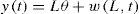
However, the system variable of interest is the flexible link tip position. So, a definition for this tip position is required in order to define the system output. Fig. 3 depicts the definition of a system output y(t), where t is the time, defined as the distance that the end effector travels along the arc of a circle of radius L centered about the joint axis of gyration.

Figure 3.

End effector position.

2.1

Finite Differences model of the PDE rotational dynamics for the Euler-Bernoulli Beam

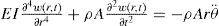
Let us consider the classical PDE of the EBB equation, in which a rotational dynamics has been included. Also, let us consider that the flexible link of the robot has its clamped base at the joint hub of the robot. This equation is a classical model in the flexible-link robots literature and can be found (e.g.) in [2] and is given by

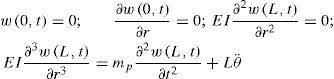
Also, it is important to define de Boundary Conditions (BC) which must be valid for the flexible link for all the time. As the Euler-Bernoulli given in Eq. 1 is fourth order in the distributed coordinate, it is necessary to define a set of four BC's. The set of BC's considered in this work corresponds to a clamped-free beam with an inertial condition at the free end, so that, they are expressed as

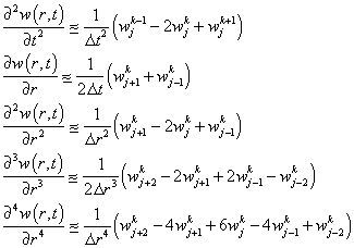
The Finite Differences Method (FDM) employs approximations to the partial derivatives found in Eqs. 1 and 2. This approximations are obtained by the discretization the domain of the variables of the PDE. A partition Δt of the time t and a partition Δr of the flexible link spatial coordinate r are required. In this way, the Finite Differences (FD) approximations needed are given by Eq. 3, which can be found in [2] and where the notation wf has been used to denote w(jΔr, kΔt) in which the quantities Δt and Δr are fixed positive constants, but, in general Δt does not equal Δr. Also, this FD approximations are generally referred to as FD analogs (see e.g. [21]). Hence,

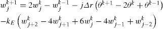
Replacing the partial derivatives in Eq. 1 by their FD analogs given in Eq. 3, it yields,

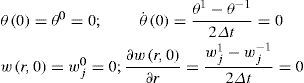
in which the initial conditions of the system at rest are

and the boundary conditions analogs are then given by

where it must be noticed the presence of fictitious points which are obtained when t = 0 (i.e., k = 0) and whenever r = 0 (i.e., j = 0) of r = L (i.e., j = n). The fictitious point of time is wj−1 whereas the fictitious points of the distributed coordinate are W−2k, W−1k and Wkn+1 with also Wkn+2. Even though these points are fictitious, they still can be calculated by solving some of the FD-BC given in Eqs. 5 and 6 or by applying these solutions to the recursive equation which goes forward in time that is obtained by solving Eq. 4 for wjk+1. Thus, by defining the constant k_E=(EIΔt²)/(ρAΔr⁴), such a recursion is found to be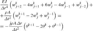

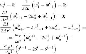
The above equations, after a not so short procedure, allow to compute both, initial and fictitious point as

and, after defining m_E=(2m_pΔr³)/(EIΔt²) and L_E=Lm_E, the last fictitious point is computed as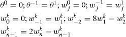

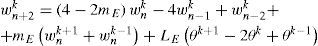
The expressions given in Eqs. 8 and 9 can now be substituted in Eq. 4 and grouped into a more compact expression for a recursive equation which represents the dynamics of the whole flexible-link robot system. Therefore, the dynamics of the overall system is,

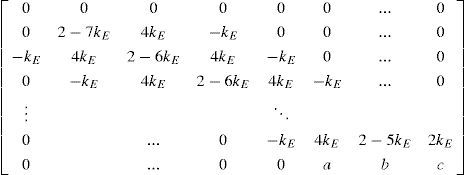
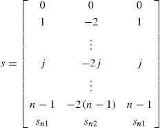
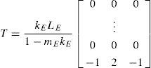
where A is (n +1 × n+ 1) and S, T are (n +1 × 3) matrices. Also, Wk=0,Wk1,Wk2, …, Wn−1,k Wn−2kT, the vector Θ=[θ^k+1, θ^k, θ^k−1]^T and the discrete coefficients a(k) and b(k) are such that, [a(0), b(0)]=[0.5, 0], and if k > 0 then, [a(k), b(k)]=[1, −1]. The actualization matrix A is given by

where a=-(2k_E)/(1-m_Ek_E), b=4k_E/(1-m_Ek_E) and the last element, c=2(1+k_E(m_E-1))/(1-m_Ek_E). Also, the matrix S is defined to be,

where the coefficients of the last row are defined to be s_n1=-n/(1-m_Ek_E) and s_n2=2n/(1-m_Ek_E). And finally,

So that, Eq. 7 allows to compute the flexible link deflection at every discretization point in the distributed coordinate r for the discrete time instant k+1 using only terms of the current time instant k and the immediate past instant k−1, which are always available. Notice however, that the required values for to compute W^k+1 are W^k, W^k−1, θ^k−1 and θ^k+1 which is a future value for the joint coordinate.

Therefore, the dynamics of the joint angle must be considered prior to the computation of Eq. 7, so that, all the needed data is available.

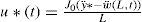
2.2

Joint dynamics in Finite Differences terms

The dynamics of the joint of the flexible-link robot (addressed as rigid mode) in the continuous time is given by

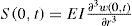
where J₀ is the rotational inertia of the joint mechanism, u(t) is the input torque driving the joint and the only available control input to the system, r_h is the perpendicular distance between the clamping of the flexible link and the rotation axis of the robot joint, and S(0, t) is the shearing force at the flexible link base, which produces the reaction torque at the joint given by the second term to the right of Eq. 14. The shearing force at the base is given by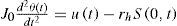

So, in order to obtain the FD analog to the rigid mode dynamics given by Eqs. 14 and 15, it is necessary to substitute the FD equivalences of the derivatives and the discretized equivalences of the functions appearing in these equations. This is a quite straightforward calculation which yields

which depends on the current and past values of the system variables. Equation 16 completes the model of the system since it allows to compute all the required data to evaluate Eq. 7, so that, it is possible to calculate W^k+1 and θ^k+1 once the initial conditions (θ⁰, W⁰) and the input torque u^k have been specified.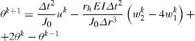

It is important to stress out that. for the FDM to work in the present case, it is necessary to obey a restriction upon the relative magnitudes of the discretization values Δr and Δt, so that, their magnitudes must be restricted to be such that,

Failure in fulfilling the restriction imposed by Eq. 17 may lead to simulation instability [21].

3

Controlling the End Effector position

The end effector position is the system variable that is required to follow a prescribed trajectory, so, let the end effector position be the output of the system which is given by (see Fig. 3)

Also, let y*(t) be the desired trajectory for the output, so that, the tracking error e and its first two time derivatives are, e=y*(t)-y(t), e˙=y˙*(t)−y˙(t)

Now, let us impose a stable dynamics upon the error and its time derivatives, so that,

where K_d and K_p are positive constants so that, Eq. 20 is Hurwitz. By substituting Eq. 19 into Eq. 20 and solving for the angular acceleration, it yields,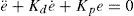

Also. from Eq. 14J0θ¨=ut−rhS0,t, but, as will be shown in the next section, the contribution of the reaction torque r_hS(0, t), to the rigid mode dynamics is negligible. This means that J0θ¨=ut. So, the error dynamics in Eq. 21 can be expressed as

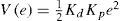
which is a perturbed first order dynamics for the error e. Let a Candidate Lyapunov Function (CLF) for the error dynamics be

which is positive definite and radially unbounded. Taking the time derivative of Eq. 23 along the trajectories of the system, it yields,

Now, define the correction angle θ*, such that

which is exactly the angular amount needed to match the current output of the system to the desired trajectory. Now, by taking the second time derivative of Eq. 25 and multiplying it by J₀, it yields,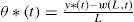

Therefore, by substituting Eq. 26 into Eq. 24 as the nominal control input, it can be seen that the time derivative of the CLF in Eq. 24 is rendered negative definite, thus, implying that the tracking of the trajectory is ideally asymptotically stable. However, the exact controlling signal u*(t) is not achieved because there always exist some parametric and modeling uncertainties. The closest thing to do, is to make sure that the rigid mode trajectory for θ(t) reaches θ*(t) as its reference trajectory. Hence, by ensuring the tracking of the trajectory θ*(t), it is possible to obtain at least, a stable trajectory tracking for the end effector position of the flexible link robot. In this work, it is also assumed that the measurement of the end effector position is available.

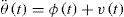
One possible way to achieve the tracking of the trajectory θ*(t) given in Eq. 25 is to employ a SMC scheme to verify that the end effector position y(t) tracks the specified trajectory y*(t). Having in mind that the rigid mode is governed by the perturbed second order dynamics Eq. 14, let us consider the first order switching function to be

where λ is a constant, and θ˜t=θt−θ*t. Also, let S(t) be a storage function, so that,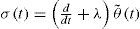

Thus, its time derivative yields

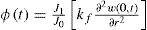
which, after some manipulations, can be expressed as

where v(t) is obtained after a control transform and φ(t) is a perturbation due to the flexible-link bending moment at the clamping, but, since the bending moment can be accurately measured, and the perturbation term φ(t) is assumed to be small and is given by

in which J₁ is the best estimation available for the system inertia moment respect to the robot joint axis, making the fraction J₁/J₀ close to 1 and k_f is a small constant in which the closeness of the sensor to the clamping and the estimate of the flexible-link stiffness are accounted for. Thus, making φ(t) a bounded function of time. Also, the control transform u(t) to v(t) is defined, so that, the rigid mode dynamics of Eq. 14 can now be expressed by

Therefore, Eq. 30 becomes

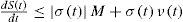
Also, the term inside the parenthesis of Eq. 33 is assumed to be bounded, that is,

so that, from Eq. 33 it turns out that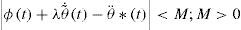

Hence, by choosing v(t) as

Then, Eq. 35 is equivalent to

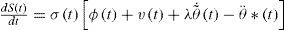
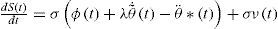
which, upon choosing M₁ > M, ensures that the rigid mode state θ,θ˙ reaches the sliding surface defined by σ(t)=0 in a finite amount of time (i.e., θ(t) reaches θ*(t) after a finite amount of time), because the time derivative of the storage function of Eq. 28 is rendered negative definite for all time. It is important to mention that the reference trajectory θ*(t) expressed in Eq. 25, can be treated as a virtual controlling signal, which can be improved by adding the classical PID gains for the error terms, so that, the improved control law for this system is given by

where K_p, K_d, K >0. Thus, the FD equivalence of Eq. 38 is then given by

also, the corresponding expression for the control law of Eq. 36 in discrete time is given by

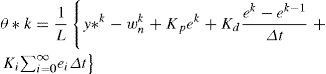
Observe from Eqs. 36 and 40 that, even though the calculations for the control law were made in terms of continuous functions of time, the controlling action given by Eq. 40 has a constant value between consecutive sampling times (which are spaced by the time amount Δt).

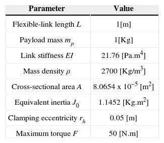
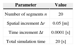
4

Simulation results

The parameters employed to simulate the control scheme devised in the last section are divided in two sets: the first one is the set of mechanical parameters of the flexible-link robot given in the Table 1, and the second set is composed by the simulation parameters needed to implement the FDM, which are given in Table 2.

Table 1.

Mechanical parameters of the robot.

Parameter	Value
Flexible-link length L	1[m]
Payload mass mp	1[Kg]
Link stiffness EI	21.76 [Pa.m^4]
Mass density ρ	2700 [Kg/m^3]
Cross-sectional area A	8.0654 x 10^−5 [m^2]
Equivalent inertia J0	1.1452 [Kg.m^2]
Clamping eccentricity rh	0.05 [m]
Maximum torque F	50 [N.m]

Table 2.

Simulation parameters for the FDM.

Parameter	Value
Number of segments n	20
Spatial increment Δr	0.05 [m]
Time increment Δt	0.0001 [s]
Total simulation time	20 [s]

The first simulation result corresponds to the regulation case where y*(t)=1.6493 [m], which is simply a constant position corresponding to a rotation angle of π/2.

The PID parameters for this regulation scheme were set to K_p=15, K_d=5, and K_i=0.1. Fig. 4 shows in dashed line the desired tip position y*(t) which is constant and in solid line the actual behavior of the end effector position which starts from a zero initial condition. Fig. 5 shows the deflection at the flexible link tip and it can be seen that it is never continuously zero. There is always a remaining vibratory effect even when the system output has reached the desired trajectory.

Figure 4.

Regulation of the end effector.

Figure 5.

Tip deflection for regulation.

Also, Fig. 6 depicts the virtual control signal θ*(t) in dashed line, whereas the actual joint angle θ(t) is shown in solid line. It is worth noticing that the angle θ(t) follows only the average of the function θ*(t), yet, the tip position has been satisfactorily regulated.

Figure 6.

Virtual control and joint angle.

The second simulation results are intended to show the flexible link robot behavior when the end effector is required to track a prescribed trajectory. For this case, the PID controller parameters were set to K_p=15, K_d=5 and K_i=1. The reference trajectory signal corresponds to the first two terms of the Fourier series of a square wave, which is given by

where the square wave period is T_s=2 [s].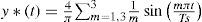

The results of the end effector trajectory tracking scheme are depicted in Fig. 7, in which it can be seen that there is always an overshot of the actual end effector position (solid line) when the reference signal (dashed line) changes its sing, but in general, the tracking of the desired trajectory is satisfactory even for the reference signal of Eq. 41, which is somewhat demanding for the flexible link robot kind. Fig. 8, on the other hand, shows that the elastic deflection at the flexible link tip presents sustained oscillations, which are significant but remain bounded though. Finally, Fig. 9 depicts a comparison between the required virtual control signal θ*(t) and the actual angular joint position d(t), whose behavior is consistent with the regulation case in that only the averaging signal of the virtual control reference is reproduced. Yet, the trajectory tracking performance of the end effector position is satisfactory.

Figure 7.

Trajectory tracking for the end effector position.

Figure 8.

Tip deflection of the flexible link for the trajectory tracking scheme.

Figure 9.

Virtual control and joint angle for the trajectory tracking scheme.

5.

Conclusions

In this paper, the modeling of a single flexible link robot was addressed using the Finite Differences Method, so that, it was possible to skip the classical Assumed Modes Method for modeling this kind of robot manipulators. Also, it was found that the trajectory of the joint driving the flexible link can be used as a virtual control signal for the system when the output is selected as the end effector position. Therefore, by defining an adequate trajectory for the robot joint in terms of the end effector position, both, system regulation and trajectory tracking for the end effector position of the flexible link were achieved. Notice however, that in this work, the calculations made to synthesize the sliding modes control law, were made using continuous time variables because a discrete time analysis and control law synthesis is currently under development including the corresponding discrete time stability analysis.