


Nowadays, in power systems, we still lack the existence of standardized test systems that can be used to benchmark the performance and solution quality of proposed optimization techniques. Several authors report that the electric load pattern is very complex. It is therefore necessary to develop new methods for design of test cases for economic analysis in power systems. Therefore, we compared two methods to generate test systems: time series model and a method simulating stable random variables based on the use of Chambers, Mallows, & Stuck (1976). This paper describes a method for simulating stable random variables in the generation of test systems for economic analysis in power systems. A study focused on generating test electrical systems through stable distribution to model for unit commitment problem in electrical power systems. Usually, the instances of test systems in unit commitment are generated using normal distribution, but the behavior of electrical demand does not follow a normal distribution; in this work, simulation data are based on a new method. For empirical analysis, we used three original systems to obtain the demand behavior and thermal production costs. Numerical results illustrate the applicability of the proposed method by solving several unit commitment problems directly and through the Lagrangian relaxation of the original problem.
The optimization problems for electrical power systems have been studied for more than five decades. One of them is the Economic Dispatch, which can be defined as the operation of generation facilities to produce energy at the lowest cost to reliably serve consumers, recognizing any operational limits of generation and transmission facilities.
Another optimization problem in power systems is the typical Unit Commitment (Wood & Wollenberg, 1996). The problem consists as determining the mix of generators and their estimated output level to meet the expected demand of electricity over a given time horizon (a day or a week), while satisfying the load demand, spinning reserve requirement and transmission network constraints. An electric network consists of many generation nodes with various generating capacities and cost functions, lines of transmission and nodes of power demand. The application of optimization models for electrical power systems is marked by constant development for new algorithms like exact methods, metaheuristics and hybrid strategies. However, to benchmark the performance and solution quality for any solution technique, it is necessary to have variety of electrical test systems.
Nowadays, we still lack the existence of standardized test systems that can be used to benchmark the performance and solution quality of proposed techniques (Ledesma-Orozco, Ruiz, García, Cerda, & Hernández, 2011; Kuo & Lin, 2013; Ding, Cai, Sun, & Chen, 2014). Many papers consider different test systems, which make it very difficult to perform a proper comparison between the different methods that have been proposed (Diniz, 2010).
(Zhang and Schaffner 2010.) refer that the existing IEEE test systems developed are mainly used for reliability, power flow and stability analysis, but not for economic analysis. Short time ago, some panels focused on the development of standard test systems of transmission and distribution systems for economic analysis has emerged. In 2007 the IEEE Working Group (WG) on Test Systems for Economic Analysis was created, sponsored by IEEE System Economics subcommittee (Zhang & Schaffner, 2010).
Finding an appropriate method for generating test cases of a specific electricity network is not an easy task. In this sense, this paper compares two methods to generate test systems: time series and a method simulating stable random variables based on the use of Chambers-Mallows-Stuck.
There are some methods to find the best estimation of load forecasting. The major methods include time series such as exponential smoothing or autoregressive integrated moving average models (ARIMA). However, the electricity demand pattern becomes more complex and unrecognized by the classical techniques used to forecast, one new alternative could be the use of stable distributions.
Lévy (1924) first developed the stable distributions theory in the 20s of last century. Since then, this distribution has been applied in different areas of knowledge, such as economics, physics, engineering and hydrology. The reason is that some phenomena of nature, like electrical demand, cannot be described assuming normal distribution. There are observations with extreme values, which characterizes the instability of the series and denotes the presence of heavy tails, and effect known as impulsivity.
Usually electrical demand presents a greater degree of impulsivity that the normal distribution cannot describe due to the presence of peaks in the series during the hours of the day and seasons of high-energy demand.
For this, we propose use Chambers et al. (1976) algorithm for simulating stable random variables characterizing demand patterns of real electrical systems. The use of Chambers et al. (1976) method for simulating stable random variables provides a new way to generate test systems widely used in power systems research. By modeling the demand using stable distribution can catch the real behavior of the electrical demand and build possible extreme scenarios, and each scenario corresponds to a price-elastic demand curve.
The simulations are based on real observations of demand for different reliability test systems. Electrical network data are taken from the 24 and 118 bus IEEE test systems (Charman, Bhavaraju, & Billington, 1979; Christie, 1993), and a portion of electric energy system of Mainland Spain (Alguacil & Conejo, 2000). Cost functions of the thermal plants data are taken from the literature. After the elaboration of these test cases, we tested a mixed integer non-linear formulation of unit commitment problem based on these cases, in order to obtain estimation about the performance of these new test systems.
Additionally, we tested the Lagrangian relaxation of the same problem to verify numerical stability of the generated test systems.
2. Stable DistributionsThe stable distributions theory was developed in the 20's of last century (Lévy, 1924). Since then, this distribution has been applied in different areas of knowledge. However, it was not until the work of Mandelbrot in the 60's that the stable distributions were popularized. Mandelbrot proposed a revolutionary theory based on this distribution to solve the problem of price fluctuations, later shown that many other economic variables follow a stable distribution (Mandelbrot, 1997).
Significantly, the stable distribution meets the Central Limit Theorem and the stability property (which denotes that stable distributions are isomorphic) that also contains the normal distribution as a special case of this. On the other hand, there is some complexity in working with such distributions, since they lack, in general, of an analytical expression. Although given recent computational advances, it is now possible to apply them with more feasibility to different areas.
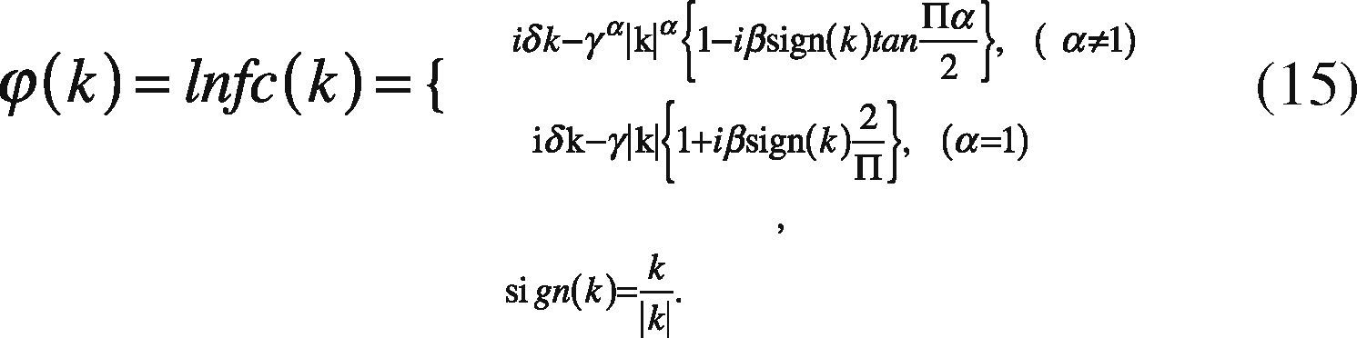
Definition: A random variable x has stable distribution having the following characteristic function (Nolan, 2005):
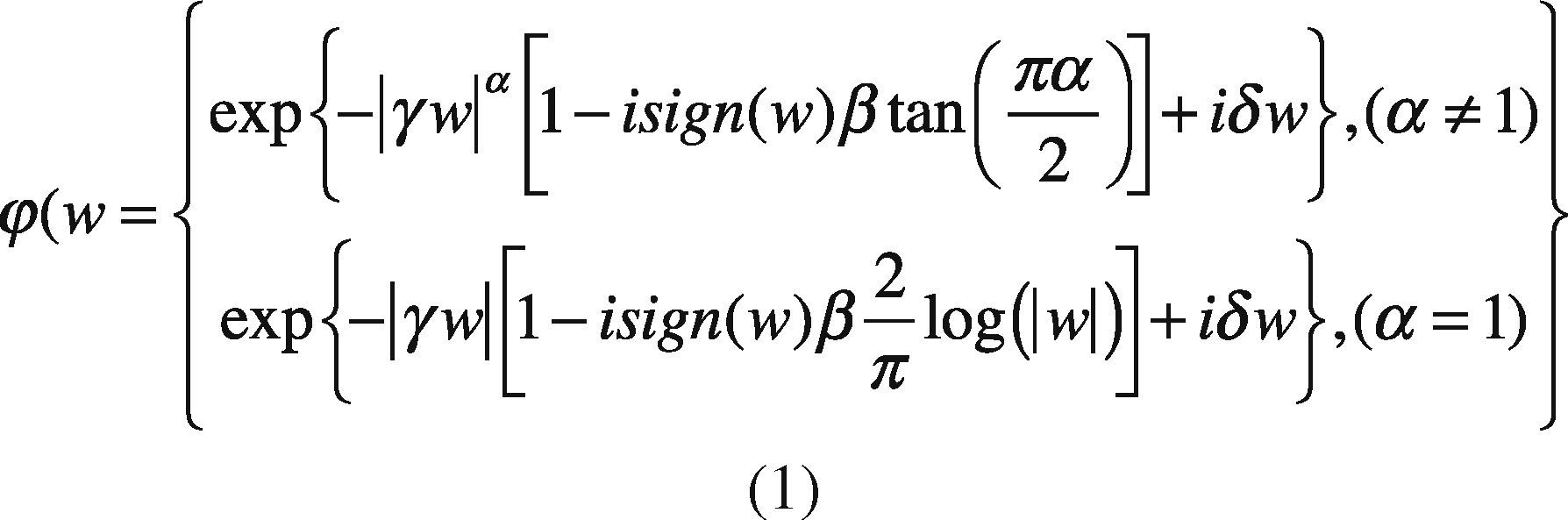
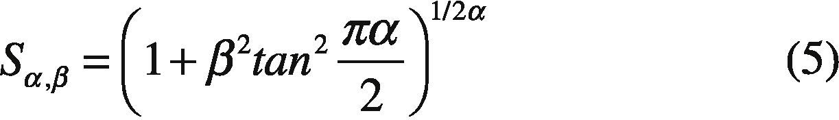
where sign(w)=w|w| and α∈ (0,2],whose parameters are defined as follows: α represents the characteristic exponent, which controls the degree of impulsiveness of the random variable w. Moreover, the parameter β ∈ [-1,+1] controls the symmetry of distribution (β = 1 and α−, distribution symmetrical, β=1 and β=-1 to the family of α distributions positive and negative respectively). While γ > 0 is a scale parameter, also called dispersion, and δ is the position parameter.
Remarkably, if the expression of the characteristic function parameter, α=2, then the parameter β becomes meaningless, since β tan π=0. In this case, the characteristic function becomes:
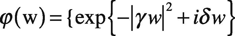
The above expression is the characteristic function of a Gaussian random variable with mean δ and variance σ=2γ2. So from the definition above, we also can show that the normal distribution is a particular case of α- distribution. Given the properties of α- distribution above, it follows that its use is justified in the same way as the Gaussian distributions and not only that, but the Gaussian distribution is a particular case of stable and therefore the range of application of α- stable distributions is even wider than the normal distribution.
This is mainly due the existence and continuity of the probability density function of α-, but with a few exceptions, it cannot be expressed in a compact way. In other words, the integral with respect to (w) of the characteristic function (1), only have an analytical solution for the described cases, denoting the α-stable distribution by four parameters fα,β,(.|γ,δ) (Nolan, 2005).
The current computational developments applied to estimate distribution parameter of α-stable distributions had been a key element in the recent use of such distributions in many areas. The statistical significance of the estimated parameters can be contrasted by the Anderson Darling test, which has been generally accepted for the analysis of stable series (Belov, Kabasinskas, & Sakalauskas, 2006).
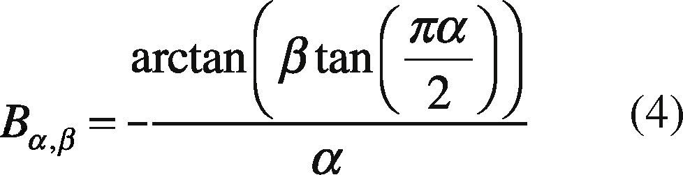
2.1. Stable Random VariableFor a random sample with α-stable distribution, the Chambers et al. (1976) method. A random variable x with distribution fα,β(X|1, 0) can be generated from a non-linear transformation of two random variables independent, one uniform (V) and another exponential (W) using the following theorem:
Theorem: Let (V) a uniform random variable in the interval −π2,ππ2 and (W) an exponential random variable with mean equal one. If (V) and (W) are independent, then:
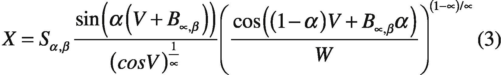
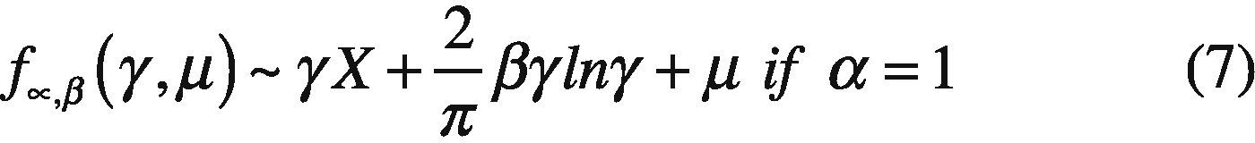
x follows a stable distribution with fα,β(X|1, 0), where:
Once you get the variable (X), a variable with stable distribution for any value of the parameters α, β, σ, μ is generated. If, X∼fα,β(X|1, 0) then:
3. The Multiperiod Unit Commitment Model
In this work we address a Multiperiod Unit Commitment (MPU) based on Marmolejo, Litvinchev, Aceves, & Ramirez (2011) notation, where network constraints are represented through a DC model (Alguacil & Conejo, 2000). The following notation is used in the mathematical model:
Constants:
Aj Start up cost of power plant j.
Bnm Subsceptance of line n – m.
Cnm Transmission capacity limit of line n – m.
Dnk Load demand at node n during period k.
Ej(tjk) Nonlinear function representing the operating cost of power plant j as a function of its power output in period k.
Ej1 Linear coefficient of operating cost for the plant j.
Ej2 Quadratic coefficient of operating cost for the plant j.
Fj Fixed cost of power plant j.
Knm Conductance of line n – m.
Rk Spinning reserve requirement during period k.
TJ¯ Maximum power output of plant j.
TJ Minimum power output of plant j.
nr¯ Reference node with angle zero.
Variables:
tjk Power output of plant j in period k.
vjk Binary variable which is equal to 1 when plant j is committed in period k.
Yjk Binary variable which is equal to 1 when plant j is started up at the beginning of period k.
δnk Angle of node n in period k.
Sets:
J Set of indices of all plants.
K Set of period indices.
N Set of indices of all nodes.
Λn Set of indices of the power plants j at node n.
Ωn Set of indices of nodes connected and adjacent to node n.
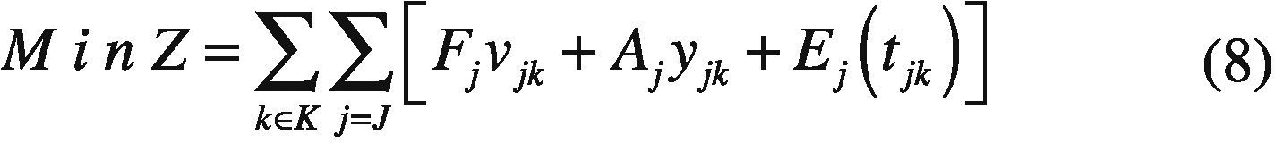
The objective is minimizing a function that includes fixed cost, start up cost and operating cost. A second order polynomial describes the variable costs as a function of the electric power.
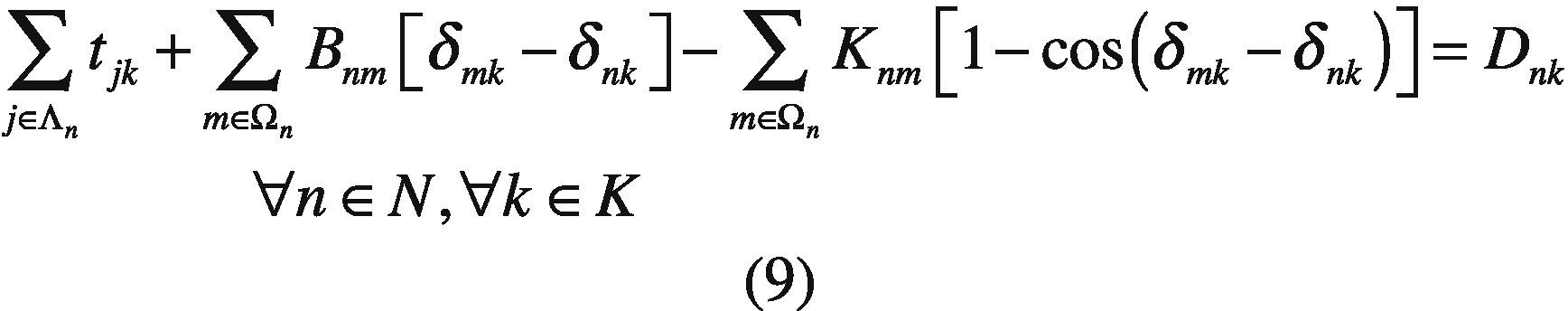
There is a power balance constraint per node and time period. In each period, the production has to satisfy the demand and losses in each node. Line losses are modeled through cosine approximation and it is assumed that the demand for electric energy is known and is discretized into t periods.
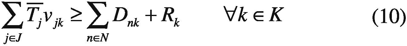
Spinning reserve requirements are modeled. In each period the running units have to be able to satisfy the demand and the prespecified spinning reserve.
Each unit has a technical lower and upper bound for the power production.

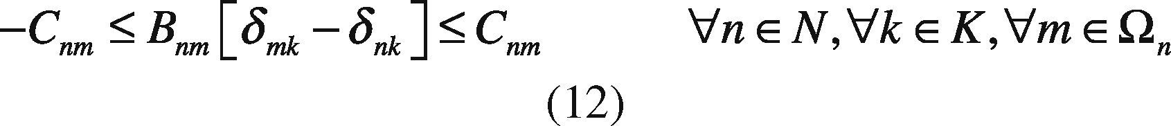
Transmission capacity limits of lines avoid dynamic stability system problems.
This constraint holds the logic of running, start-up and shut-down of the units. A running unit cannot be started-up.

Angle in all buses has a lower and upper bound.

4. Test Systems Generation
To generate new test systems (instances) by the proposed methods, we worked with three standardized test systems:
- •
SYS-104: Based on 104-bus electric energy system of Mainland Spain with 104 nodes, 62 thermal units and 160 transmission lines (Alguacil & Conejo, 2000).
- •
IEEE-24 bus test system with 24 nodes, 24 thermal units and 38 transmission lines (Charman et al., 1979).
- •
IEEE-118 bus test system with 118 nodes, 54 thermal units and 186 transmission lines (Christie, 1993).
All instances consider a 24-hour planning horizon with one period per hour.
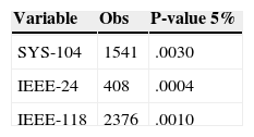
4.1. Stable DistributionKolmogórov-Smirnov normal test show that three systems do not follow a normal distribution, and for the nature of the series have a fat tails characteristics (Table 1). For that reason, we use alpha stable distribution to fit the data. It was felt that S1 parameterization it is usually used for modeling stable data (Samorodnitsky & Taqqu, 1994).
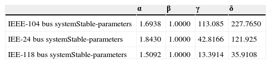
Data setting parameters were obtained characterizing the distribution by regression method (Nolan, 1999). This method is generally used in the analysis of stable series that has a better adjustment of the tails of the distribution (Table 2).
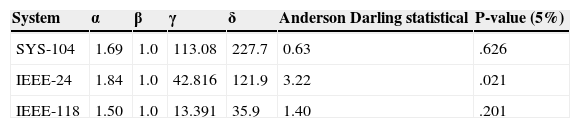
To test the fit of the distribution to data, many authors agree with the utility of Anderson-Darling test for data with fat tails (Stephens, 1977). For all cases, the null hypothesis was not rejected (Table 3). The parameter alpha in three systems shows the presence of impulsivity, all series are symmetric positive, and have high dispersion. That depend the demand in the 24 hours of day and shows the habits of consumption.
The effect of parameter alpha in the distribution function fitted is showed in the Figure 1 The parameter alpha measure the impulsivity of data that the reason because is one of the most important parameters for this analysis.

With the parameters estimated and using Chambers et al. (1976) method were created 300 instances for each original test system according to the original energy demand range. The numerical behaviors of some of these instances are showed in the next section.
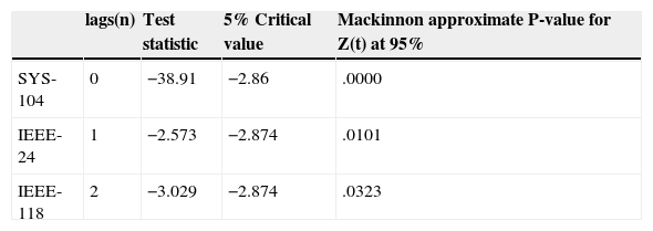
Additionally, three ARIMA models were estimated to compare two methods to generate demand data for the three systems analyzed. Dickey Fuller test was performed for stationary test series. For SYS-104 system, data series is stationary in levels, IEEE-24 system is stationary in first difference and IEEE-118 is stationary in second difference (Table 4).
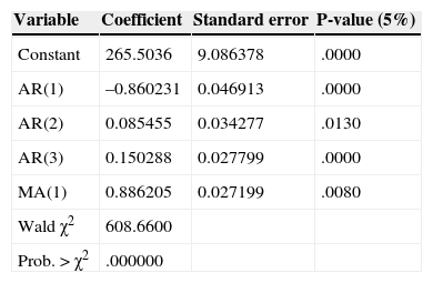
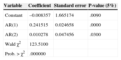
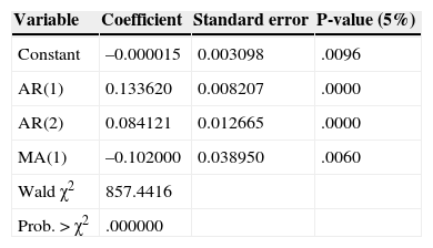
The adjustment of the three models, shows components autoregressive (p) and moving average (q). Tables 5–7 show the estimates of the models. Based on the time series models for the three systems, were forecast 50 observations of each one. One of the main limitations of using ARIMA models for generating test systems is that each model is a specific case, so it is not possible to generalize results.
From the initial values of (p) and (q) definition, several alternative models with various combinations AR (p) and MA (q) are proposed. The proposed models are compared to each other using the value of the coefficients and criteria of Akaike (AIC) and Schwarz (SC).
5. Solving StrategiesGenerated test systems can be used to benchmark the performance and solution quality in several solving strategies. In this work, we compare the direct solution through GAMS and Lagrangian Relaxation (LR) of the problem. Through LR we can obtain a lower bound on the value of the objective function of the original problem.
LR decomposes the original problem into a Dual Master Problem and makes better and easily manageable Dual Subproblems to be solved separately. Lagrange Multipliers that are added to the master problem to yield a dual problem link the subproblems. The dual problem has lower dimensions than the primal problem and is easier to solve. The multipliers are updated through different methods; in this work, we use subgradient method. The major difficulty of this method is associated with obtaining solution feasibility, because of the dual nature of the algorithm.
Dual Master Problem:
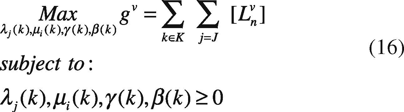
Dual Subproblem:
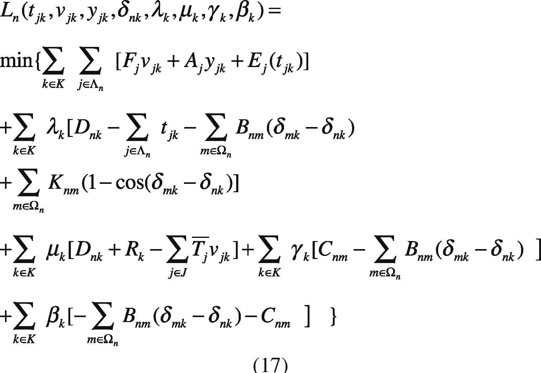
Subject to Eqs. (11), (13), and (14).
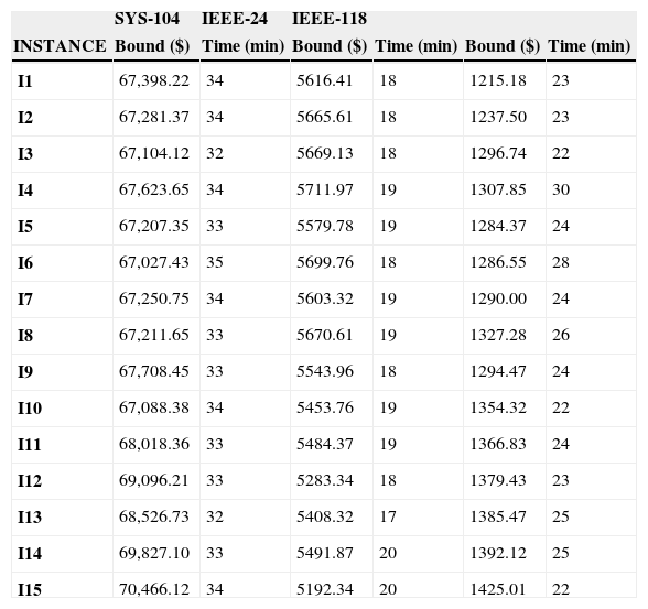
6. Computational ResultsIn this section we present the results to the computational experiments that we carried out to evaluate the performance of the generated test systems by the proposed method (Figures 2–7). All simulations and mathematical models were carried out on an AMD Phenom™ II N970 Quad-Core with a 2.2GHz processor and 4 GB RAM. Table 8 (Brooke, Kendrick, & Meeraus, 2010b) shows the results of the MPU for 20 generated instances by DICOPT solver.


Results obtained by DICOPT Solver.
| SYS-104 | IEEE-24 | IEEE-118 | ||||
|---|---|---|---|---|---|---|
| INSTANCE | Bound ($) | Time (min) | Bound ($) | Time (min) | Bound ($) | Time (min) |
| I1 | 67,398.22 | 34 | 5616.41 | 18 | 1215.18 | 23 |
| I2 | 67,281.37 | 34 | 5665.61 | 18 | 1237.50 | 23 |
| I3 | 67,104.12 | 32 | 5669.13 | 18 | 1296.74 | 22 |
| I4 | 67,623.65 | 34 | 5711.97 | 19 | 1307.85 | 30 |
| I5 | 67,207.35 | 33 | 5579.78 | 19 | 1284.37 | 24 |
| I6 | 67,027.43 | 35 | 5699.76 | 18 | 1286.55 | 28 |
| I7 | 67,250.75 | 34 | 5603.32 | 19 | 1290.00 | 24 |
| I8 | 67,211.65 | 33 | 5670.61 | 19 | 1327.28 | 26 |
| I9 | 67,708.45 | 33 | 5543.96 | 18 | 1294.47 | 24 |
| I10 | 67,088.38 | 34 | 5453.76 | 19 | 1354.32 | 22 |
| I11 | 68,018.36 | 33 | 5484.37 | 19 | 1366.83 | 24 |
| I12 | 69,096.21 | 33 | 5283.34 | 18 | 1379.43 | 23 |
| I13 | 68,526.73 | 32 | 5408.32 | 17 | 1385.47 | 25 |
| I14 | 69,827.10 | 33 | 5491.87 | 20 | 1392.12 | 25 |
| I15 | 70,466.12 | 34 | 5192.34 | 20 | 1425.01 | 22 |
For LR, we use the solver DICOPT for solving the MINLP problems (dual subproblems), CONOPT for solving the NLP problems (primal subproblems), and CPLEX for MIP problems (master primal problem) (Brooke, Kendrick, & Meeraus, 2010a).
Concerning the computational times, we note that they are similar than original systems. In general, the generated instances do not have numerical problems in the optimization process, which normally occurs in Unit Commitment Problem.
7. ConclusionsNowadays, we still lack the existence of standardized test systems that can be used to benchmark the performance and solution quality of proposed techniques.
Several authors report that the electric load pattern is very complex. It is therefore necessary to develop new methods. Therefore, we compared two methods to generate test systems. However, we found that the time series methods perform poorly due to the limited capacity to generate new data and the specificity of the results. The results show that the method of stable distributions generate better test systems than those caused by time series. By using the stable distribution, setting data is more accurate and the range of values that can be generated is unlimited.
By introducing Chambers et al. (1976) method, we presented a new way to generate electrical test systems for economic analysis. We show that the electrical demand fits a stable random variable, so we use it to generate several instances for the original test systems.
Electrical demand presents a greater degree of impulsivity due to the presence of peaks in the series during the hours of the day and seasons of high energy demand.
By modeling the demand through the use of alpha stable distribution can catch the real behavior of the electrical demand and build possible extreme scenarios, each scenario corresponds to a price-elastic demand curve.
We test all generated instances in the Multiperiod Unit Commitment Problem and the LR. The results show that the proposed methodology is relevant, obtaining feasible solutions with GAMS (Brooke, Kendrick, & Meeraus, 1998) solver in the same way of the original systems.
This work contributes to have standardized test systems that can be used to benchmark the performance of many proposed techniques.