


The financial crisis that began in late 2007 has raised awareness on the need to properly measure credit risk, placing a significant focus on the accuracy of public credit ratings. The objective of this paper is to present an automated credit rating model that dispenses with the excessive qualitative input that, during the years leading to the 2007 crisis, may have yielded results inconsistent with true counterparty risk levels. Our model is based on a mix of relevant credit ratios, historical data on a corporate universe comprising the global pharmaceutical, chemicals and Oil & Gas industries and a powerful clustering mathematical algorithm, Self-Organising Maps, a type of neural network.
La crisis financiera que comenzó a finales de 2007ha incrementado la concienciación sobre la necesidad de medir adecuadamente el riesgo del crédito, haciendo mayor hincapié en la precisión de las calificaciones públicas. El objetivo de este trabajo es presentar un modelo automatizado de calificación crediticia que prescinda del exceso de lo cualitativo, habitual durante los años previos a la crisis de 2007, y que pudo haber provocado resultados inconsistentes con los niveles reales del riesgo de crédito. Nuestro modelo se basa en una combinación de las ratios crediticias relevantes, los datos históricos relativos a un universo empresarial que incluye a las industrias farmacéuticas, químicas y petrolíferas, y un potente algoritmo matemático de agrupación, SOM, que constituye un tipo de red neuronal.
During the last few decades, particularly since the late 1980s, the development and growth of international debt capital markets have been linked to public credit ratings, where these credit risk assessments were provided by a handful of approved rating agencies, which still today enjoy an oligopolistic market position. As industries and companies active in bond markets grew in number and complexity, so did the way rating agencies approached the once mostly quantitatively-driven credit analysis they offered. Over time, qualitative inputs were incorporated in order to fine-tune credit ratings to the most appropriate level, admittedly resulting, in general, in an improvement in the accuracy and timeliness of ratings and rating changes. At least it did so until the weight of qualitative information came to grossly outweigh quantitative analytics.
The excessive use of qualitative considerations in credit ratings may have caused an increase in the amount of credit rating cliffs in recent years, that is, multi-notch downgrades that cannot only be explained by the evolution of the global recession which began in 2007. Recently, rating changes in the 5 to 10-notch range within 12-month periods have been common in sovereign, banking, structured and corporate ratings.1 Our hypothesis is that a significant increase in the weight of quantitative inputs in the future assignment of public credit ratings is now warranted, particularly since ratings have become an instrument of regulation, and are therefore critical for the correct operation of debt markets. As described by Arrow and Debreu, “rating agencies fulfil a mission of delegated monitoring for the benefit of investors active in bond markets”. As such, they must be accurate.
This paper purports to explore a particularly powerful and reliable quantitative rating methodology, which aims to measure the relative creditworthiness of bond issuers at senior bond level, providing an accurate and reliable distribution or relative ranking of credit risk. This should be done without excessive interference from human judgement because, whilst judgement allows for fine-tuning, in our view it should never be the only underpinning of a credit opinion. We will propose the use of Self-Organising Maps (SOMs), a type of neural network which can be analytically audited, as the basis for the establishment of relative credit rankings of issuers within and across sectors globally.
2Credit ratings and the focus on qualitative analysisFirst, we must review the basics. What are credit ratings and how did they first appear in debt capital markets?
According to Arnaud de Servigny and Renault (2004), “Standard & Poor's perceives its ratings primarily as an opinion on the likelihood of default of an issuer, whereas Moody's Investors Service's ratings tend to reflect the agency's opinion on the expected loss (probability of default times loss severity) on a facility”. However, to put it bluntly, with the exception of ratings in the structured finance field, public ratings are nothing more than a relative ranking of credit. The expected loss on a credit position can be more accurately assessed in retail credit (for example, on a consumer personal loan), mainly due to the existence of historic default data by vintage on homogeneous pools of assets. This is not possible in corporate credit, and therefore what all agencies actually aim to achieve is a relative credit ranking across sectors and countries.
Credit ratings were first introduced in the US bond market in 1909, when John Moody published debt ratings on some 250 major railroads. The relative ranking of credit quality was assessed quantitatively and simply placed on a ratings book that would thereafter be published annually. Within a few years, other rating organisations appeared, some of them merging soon after to form Standard & Poor's, the other major player in the ratings industry. The ratings universe soon expanded to include industrial and municipal bonds, as well as sovereign and international corporate issuers active in the US bond markets. By the early 1930s, the US bond market had over 6000 published bond ratings, with nominal amounts exceeding $30 billion. The rating agencies’ business thrived.
Particularly since the late 1970s, a whole array of lending options has emerged for thousands of borrowers spread throughout the globe, underpinned by a secular growth in debt securities and, with it, a growing demand for credit risk analysis. Today, three large rating agencies, Standard & Poor's, Moody's Investors Service and Fitch Ratings, control the vast majority of public ratings, with a fourth one, DBRS, catching up quickly. All have evolved from a mainly quantitative analysis, to an increasingly qualitatively driven methodology.
The objective of credit analysis is to forecast the capacity and willingness of a debt issuer to meet its obligations when due. It is, therefore, an exercise which aims to predict the future as accurately as possible. It also seeks to maintain, to the extent possible, a low volatility in rating levels. That is, it tries to see through economic cycles, keeping ratings stable by avoiding excessive downgrades during downturns and excessive upgrades in booming economic times.
As the physicist Niels Bohr once said, “It's tough to make predictions, especially about the future”. Rating agencies have struggled over time to ensure a robust methodology is used to predict future events. At a certain point in time, financial ratios and cash flow estimates were deemed insufficient to estimate the behaviour of an aggressive management team, the likely actions of a particular shareholder in financial distress, or the monopolistic status of a particular company. Qualitative input was seen as inevitable; sound judgement from credit analysts, necessary (Dwyer and Russell, 2010).
Moody's Investors Service, to name one of the two largest rating agencies, in its publication “Global Credit Analysis”, chapter 8 (IFR Publishing, 1991), underscores the qualitative aspects of analysis in predicting the future. It asserts that “in practice, the job of assessing the size and predictability of a company's “cash buffer” begins -and ends- with a qualitative assessment of factors that will have an impact on that buffer over time. This is where the most analytical energy is spent”.
In fact, we know from agencies’ manuals that they make a substantial amount of rating adjustments to reflect issues such as the perceived quality of issuers’ senior management teams, the degree of risk aversion expected from issuers’ middle management, the potential for increased volatility in operating environments, the perceived sustainability in the quality of products and services offered by a rated entity, or the expectation of prompt government support for certain rated banks in a potential banking crisis. All of the above are qualitative factors and considerations which do, ultimately, shift rating outcomes derived from pure quantitative considerations.
Whilst we accept this, we must also note that qualitative information is already contained in a great deal of financial ratios and figures. For example, relative size can be an indirect indication of the likely external support an issuer may receive; a borrower's capital structure gives clues regarding management's risk tolerance; average ratios in particular sectors provide indirect information regarding a sector's competitive landscape. These quantitative indicators do already, therefore, contain a very fair amount of qualitative meaning, and are less likely to be impacted by errors in human judgement. The artificial creation of “rating floors”, for example, which are rating levels below which a specific credit rating should not be assigned (due, entirely, to assumptions of external support), are dangerous judgmental practices based on purely qualitative considerations.
Traditionally, large deposit-taking financial institutions and corporates in key sectors of the economy, as well as some smaller sovereigns, have been the usual beneficiaries of excessively high credit ratings, strongly supported by qualitative factors alone (such as, for example, the expectation of a government bailout). However, whilst that expectation made sense for UBS, it did not for Lehman. Or take the example of Iceland's triple-A rating, underpinned by the expectation of a strong “willingness” to pay, a qualitative consideration at the expense of an appropriate analysis measuring the country's “capacity” to pay, a quantitative exercise. More quantitatively-driven rating methodologies would perhaps increase ratings’ predictive capacity and result in less abrupt rating moves on the back of adverse economic scenarios. Note that it is generally accepted by rating agencies that a rating error occurs when an Investment Grade issuer defaults or is downgraded more than twice within a 12-month period. It is, therefore, unquestionable that rating errors have been far too plentiful in recent times, perhaps more than would have been expected. This is a reflection on the excessive use of “optimistic” qualitative inputs in credit analysis.
As a final consideration on the usefulness of transparent quantitatively-driven rating methodologies, note that such methodologies would most likely help dispel the mistaken idea that conflicts of interest between rating agencies and paying issuers force higher ratings overall. There is no evidence of such behaviour, but doubt remains in the bond marketplace. Furthermore, the fact that, since the mid-1970s, agencies’ published ratings have become an element of regulation has greatly distorted the sector, generating conflicts of interest that thrive in a highly judgmental analytical environment (Bolton et al., 2012). As Goodhart's Law puts it, “once a financial indicator is made a target for the purpose of conducting financial policy, it will lose the information content that would qualify it to play that role”. While rating agencies have admittedly weathered these conflicts well, the use of independent and judgmentally neutral quantitative rating tools would help counterbalance those conflicts. In this context, SOMs provide a powerful and robust analytical framework for credit, one that would serve the agencies well alongside their traditional rating methodologies.
The relative ranking of these credit views are expressed along the following scale (Fig. 1), from most creditworthy, to least creditworthy, in relative terms.
3Selection of suitable ratios
There is no general agreement regarding which ratios are best for credit rating purposes, nor is there any generally accepted theory indicating the most suitable ratio selection (Dieguez et al., 2006). For example, for Ohlson (1980) the representative variables are size, financial structure, results and liquidity, whereas Honjo (2000) considers that capital structure and size are good predictors of business failure, and Andreev (2006) focuses on liquidity (working capital) and return (operating margin) as key variables to predict business failure.
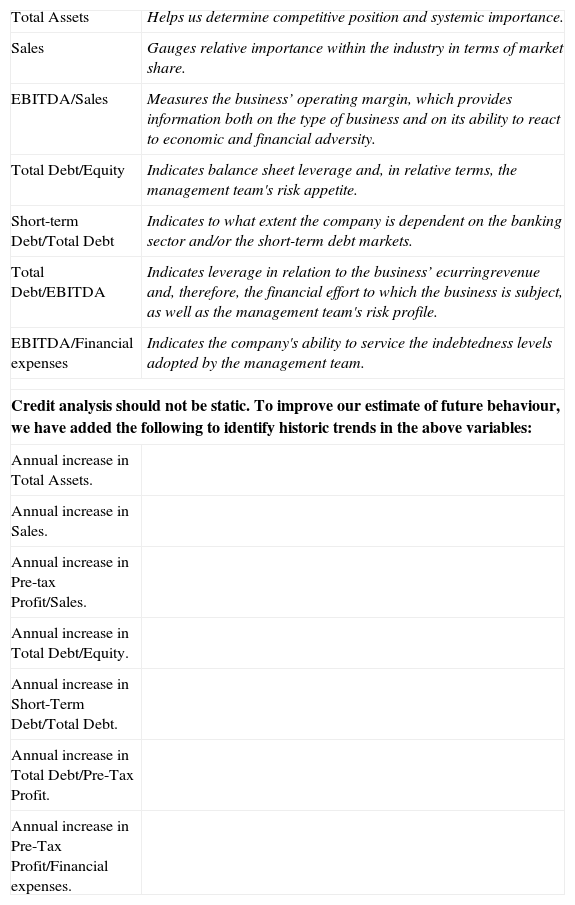
Based partly on a paper by Moodys (2007), we have selected 14 variables (Table 1) broadly used by credit analysts, of which the first two are absolute variables and the 3rd to the 7th are credit ratios; variables 8–14 reflect increases in the first seven variables.
Variables used by the model.
| Total Assets | Helps us determine competitive position and systemic importance. |
| Sales | Gauges relative importance within the industry in terms of market share. |
| EBITDA/Sales | Measures the business’ operating margin, which provides information both on the type of business and on its ability to react to economic and financial adversity. |
| Total Debt/Equity | Indicates balance sheet leverage and, in relative terms, the management team's risk appetite. |
| Short-term Debt/Total Debt | Indicates to what extent the company is dependent on the banking sector and/or the short-term debt markets. |
| Total Debt/EBITDA | Indicates leverage in relation to the business’ ecurringrevenue and, therefore, the financial effort to which the business is subject, as well as the management team's risk profile. |
| EBITDA/Financial expenses | Indicates the company's ability to service the indebtedness levels adopted by the management team. |
| Credit analysis should not be static. To improve our estimate of future behaviour, we have added the following to identify historic trends in the above variables: | |
| Annual increase in Total Assets. | |
| Annual increase in Sales. | |
| Annual increase in Pre-tax Profit/Sales. | |
| Annual increase in Total Debt/Equity. | |
| Annual increase in Short-Term Debt/Total Debt. | |
| Annual increase in Total Debt/Pre-Tax Profit. | |
| Annual increase in Pre-Tax Profit/Financial expenses. | |
Artificial neural networks were originated in the 1960s (Minsky & Papert, 1969; Rosenblatt, 1958; Wildrow and Hoff, 1960), but began to be used in the 1980s (Hopfield, 1984; Kohonen, 1982) as an alternative to the prevailing Boolean logic computation.
Basically, there are two kinds of neural networks: supervised and Self-Organising Networks. The former are universal function “approximators” (Martín and Sanz, 1997; Funahasi, 1989), used both to adjust functions and to predict results. The latter are data pattern classification networks. These kinds of networks discover similar patterns within a pool of data and group them based on such similarity (Martín and Sanz, 1997). They are used in a wide range of activities (Hertz et al., 1991).
The first Self-Organising Networks were so-called “competitive networks”, which include an input and an output layer. Each layer comprises a group of cells. Model inputs are introduced through the input layer cells. Each cell in the input layer is connected to each of the cells in the output layer by means of a number, called a synaptic weight (Fig. 2) (Willshaw & Malsburg, 1976).

The goal of the network is to find out which cell in the output layer is most similar to the data introduced in the input layer. For this purpose, the model calculates the Euclidean distance between the values of the input layer cells and the values of the synaptic weights that connect the cells in the input layer to those of the output layer.
The cell in the output layer that shows the least distance is the winner, or best-matching unit (BMU), and its synaptic weights are then adjusted using the learning rule, to approximate them to the data pattern in the input cells. The result is that the best matching unit has more possibilities of winning the competition in the next submission of input data; or fewer if the vector submitted is different. In other words, the cell has become specialised in this input pattern.
Kohonen (1982, 1989, 1990, 1997) introduced the neighbourhood function to competitive networks, creating so-called Self-Organising Feature Maps or SOMs. Kohonen's innovation consisted in incorporating to the winning cell a neighbourhood function that defines the surrounding cells, altering the weights of both the winning cell and of other cells in the neighbourhood thereof. The effect of introducing the neighbourhood function is that cells close to the winning cell or BMU become attuned to the input patterns that have made the BMU the winner. Outside the neighbourhood, cell weights remain unaltered. For an SOM-type Self-Organising Network to be able to classify, it must have the capacity to learn. We divide the learning process into two stages:
- 1.
Classification, to identify winning neurons and neighbouring neurons.
- 2.
Fine adjustment, to specialise winning neurons.
The mechanics of Self-Organising Maps begin by allocating random weights Wijk to link the input layer and the output layer. Next an input data pattern, X(t), is introduced, and each neuron in the output layer calculates the similarity between its synaptic weight and the input vector, by means of the Euclidean Distance2 represented in Eq. (1).
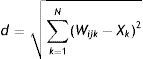
The output network neuron that shows the least distance to the input pattern is the winning neuron, g*. The next step is to update the weights corresponding to the winning neuron (Wijk) and its neighbours, using the following equation:
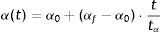
where α(t) is a learning term, which takes values comprised between 0 and 1. Where the number of iterations exceeds 500, then α(t) tends to 0. Eq. (3) is usually used to calculate α(t).where α0 is the initial rate, αf the final rates, which usually takes values amounting to 0.01, t is the current situation and tα is the maximum number of desired iterations.
The function h(|i−g*|, t) is the neighbourhood function, and its size is reduced in each iteration. The neighbourhood function depends on the distance and on the neighbourhood ratio. This function tells us that the neighbourhood function decreases when the distance to the winning cell increases. The further away from the winning neuron, the smaller the cell's neighbourhood function. It depends on the neighbour ratio R(t), which represents the size of the current neighbourhood.h(1−g*,t)=f[R(t)]
To calculate neighbourhood, step functions or Mexican hat-type functions are used. The neighbour ratio R(t) decreases in time. Below is a commonly used equation that reduces the neighbour ratio in time:(4)R(t)=R0+(Rf−R0)⋅ttRRf is the final ratio, which takes a value equal to 1. Likewise, tR is the number of iterations required to reach Rf.
In the fine adjustment stage, α is equal to 0.01, and the neighbourhood ratio is equal to 1. The number of iterations is proportional to the number of neurons, and separate from the number of inputs. Usually, between 50 and 100 iterations are sufficient.
The greater the number of identical patterns, the greater the number there will be of neurons that specialise in such pattern. The number of neurons specialised in recognising an input pattern depends on the likelihood of such pattern. The resulting map therefore approaches a probability density function of the sensory space. The amount of neurons concentrated in a certain region shows the greater likelihood of such patterns.
After declaring which is the winning neuron (Best-Matching Unit, BMU), the SOM's weight vectors are updated, and their topological neighbours move towards the input vector, thus reducing the distance. This adaptation generates a narrowing between the winning neuron and its topological neighbours in respect of the input vector. This is illustrated in Fig. 3, where the input vector is marked by an X. The winning neuron is marked with the acronym BMU. Observe how the winning neuron and its neighbours get closer to the input vector. This displacement is reduced to the extent that the distance from the BMU is greater.
 and its neighbours, moving them towards the input vector, marked by an X. Continuous lines and dotted lines respectively represent the situation before and after the update.")
Updating of the winning neuron (BMU) and its neighbours, moving them towards the input vector, marked by an X. Continuous lines and dotted lines respectively represent the situation before and after the update.
SOMs are especially useful to establish unknown relations between datasets. Datasets that do not have a known preset order can be classified by means of an SOM network. Serrano and Martin (1993)’s pioneering work on the use of artificial neural networks focuses on analysing predictions of bank failures. Mora et al. (2007) have found that, by using Kohonen's SOM effort and the U-Matrix to predict business failure, the variables obtained are in accordance with the variables obtained after using more complex parametric and non-parametric tests, which are more difficult to use.
5The modelA common problem is the complex nature of large groups of data. When a rating agency wants to evaluate different companies, it avails itself of many financial characteristics. Kohonen's Self-Organising Networks (SOM) can project an n-dimensional database on a 2-dimensional map, making it possible to find relationships derived from the underlying data.
Contrary to other neural networks, SOM is not a black box. SOM is the projection of a non-linear plane drawn from observations. The form of the plane is set using a very strict and clear algorithm, and when the algorithm is completed the form of the plane is fixed.
We can employ SOM in two ways, to give an accurate description of the data set, and to predict values.
The goal of this paper is to develop a model to classify businesses based on the likelihood of insolvency. For these purposes, we use the 14 inputs defined in Table 1. We have used a database from 2002 to 2011 comprising 402 businesses in the oil, pharmaceutical and chemical industries, including 34 companies that, at the time of the study, were immersed in bankruptcy proceedings.
This model's development begins by defining the edges of the scale of credit ratings to be used; bankrupt companies shall be rated “C” while the most solvent companies shall be rated “AAA”. This is why the model requires a number of bankrupt companies and companies that, as a result of their size, market dominance, sustainable and significant profit margins, low indebtedness and conservative management profile, are awarded the maximum rating.
The 2-D map obtained by SOM places the companies included in the database in clusters, based on the 14 inputs used. The defined 2D map has 99cells in an 11×9 pattern; we shall name each cell by its respective column number, counted from the first cell topographically located on the top right-hand corner, as shown in Fig. 4A. Once the database is defined, we train the network.

The result of training the neural network is the distribution of companies in the 2D map shown in Fig. 4B. The model places several companies in the same cell when their inputs are the same. Companies located in nearby cells have similar inputs; depending on the degree of similarity of the companies’ inputs, the companies shall be placed in cells that are closer or further away from each other. This “neighbourhood” indicates that companies located in the adjacent cells show similar credit features. The length of the columns in Fig. 4B represents the number of companies on each cell.
In order to establish the location of the extremes of our model we filter all companies, leaving only bankrupt and AAA-rated companies. The positions of these two sets of companies are observed in Fig. 5. The rating model has placed bankrupt companies around cell no. 1, whereas AAA-rated companies are placed in cell 11.

The neural network has specialised each cell in a specific credit rating. The rating extremes are located in cell 1 and in cell 11 and the database companies are distributed among the remaining cells depending on their inputs.
This map is therefore, in itself, a credit-based classification of the companies, where they are rated based on their similarity. Each company's position in the map will indicate its distance to cell 1, which shall serve to give it a rating. To the extent that the company's figures should deteriorate, its distance from the bankruptcy area will decrease, and the model will place the company in a cell closer to cell 1.
The model shows an underlying order: following the neighbourhood principle, the similarity between cells decreases as the distance between them increases. This implies increasing distances in respect of the benchmark cell. We shall take as benchmark cell no. 1, which hosts a set of bankrupt companies, and calculate the Euclidean distances between this cell and the remaining cells in the 2D map in order to establish the respective distance between each of the cells in the rest of the 2D map and the cell representing bankruptcy. Having obtained these calculations, we normalise them to a range of 0–100. The longest distance, 100, is the distance between cell no. 1 and cell no. 11.
Finally the companies shall be ranked based on their distance from bankruptcy: a credit rating of the companies is thus obtained.
The numbers shown in the different cells in Fig. 6 represent normalised Euclidean distances to cell 1. After a company's data are entered in the model, the company is placed in a cell showing the distance to cell no. 1. Knowing that cell no. 1 represents bankruptcy, and that cell no. 11 represents the best rating and is at the furthest distance from the former, a distance of 100, the different companies’ location in the map represents their credit rating. Each company is placed in a cell together with other companies showing similar features. The distances shown refer to distance from the bankruptcy area. The lower the distance, the greater the similarity to the companies located within the bankruptcy area.

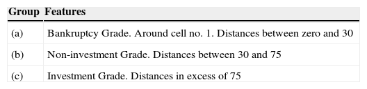
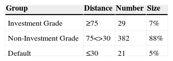
By observing the distances we may distinguish three large groups: the bankrupt companies are located in the group a, while the companies with AAA rating and the Investment Grade are in group c. Consequently, Non-Investment Grade companies are located in group b, as shown in Table 2:
Fig. 6B shows normalised distances on three axes. When the distances are represented in a 3D chart, slopes and valleys are formed. The slopes reflect large variations in distances, while in valleys distances vary only slightly. The two slopes observed in the map coincide with the areas in which are located the set of bankrupt companies, on the one hand, and Investment Grade companies, on the other.
We shall call delta the variation in the normalised distance (NED) where the number of the cell (U) changes.

As mentioned above, Delta is much higher in groups a (Bankruptcy) and c (Investment Grade) than in group b (Non-Investment Grade). This means that the change in normalised Euclidean distances is greater in the group of bankrupt companies and Investment Grade companies. This indicates that the companies included in the bankrupt group find it more difficult to get out of this group. On the other hand, the high delta shown by the Investment Grade group indicates that it is difficult for companies rated Non-Investment Grade to become Investment Grade.
To obtain the above distribution, the model has distributed the 14 inputs in the 2D map. If we analyse the 14 inputs one by one, we obtain map distributions for each of them, as shown in Fig. 7

The first 2D map in Fig. 7 is a unified distance matrix (U-matrix) indicating the Euclidean distance between each cell and its neighbours. Dark areas indicate very short distances, while lighter cells indicate greater distances. It shows how group (b) has very short distances between cells. This means that companies included in this area are very similar to each other. In both the bankruptcy area and in the AAA-rated area, distances between cells are higher, a reflection of the fact that there are fewer companies; this is why distances are greater. The U-Matrix confirms our perception of the existence of three groups or clusters.
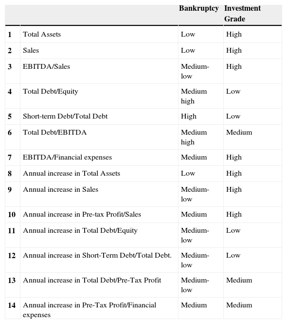
The remaining 2D maps in Fig. 7 shows the distribution of the model's inputs. Letter H indicates that the input shows its highest levels in this area, while letter L indicates the lowest levels. By observing them we can deduce the different features of the three areas. Table 3 shows the differences between groups a (Bankruptcy) and c (Investment Grade). The greatest differences are found in absolute values and ratios. However, increases show more subtle differences.
Comparison between the level of each variable in Bankruptcy and Investment Grade areas.
| Bankruptcy | Investment Grade | ||
|---|---|---|---|
| 1 | Total Assets | Low | High |
| 2 | Sales | Low | High |
| 3 | EBITDA/Sales | Medium-low | High |
| 4 | Total Debt/Equity | Medium high | Low |
| 5 | Short-term Debt/Total Debt | High | Low |
| 6 | Total Debt/EBITDA | Medium high | Medium |
| 7 | EBITDA/Financial expenses | Medium | High |
| 8 | Annual increase in Total Assets | Low | High |
| 9 | Annual increase in Sales | Medium-low | High |
| 10 | Annual increase in Pre-tax Profit/Sales | Medium | High |
| 11 | Annual increase in Total Debt/Equity | Medium-low | Low |
| 12 | Annual increase in Short-Term Debt/Total Debt. | Medium-low | Low |
| 13 | Annual increase in Total Debt/Pre-Tax Profit | Medium-low | Medium |
| 14 | Annual increase in Pre-Tax Profit/Financial expenses | Medium | Medium |
The last map shows the position of all three groups: a (bankrupt companies), c (AAA-rated companies) and b (remaining companies).
Companies located within the bankruptcy cluster show low asset values compared to the overall sample, and a low level of sales and investments; this is deduced from their low levels of asset increases. They also present large cost structures in connection with sales, as measured by their EBITDA/Sales ratio. Moreover, they are overleveraged and their debt is of poor quality, as most of it is short-term, which may cause cash shortages.
Contrary to the most commonly used credit rating models, our model has 101 ratings, from 0 to 100, that can be summarised in three groups, as indicated in Table 1. To analyse the model's distribution of credit ratings, we have constructed a frequency histogram, represented in Fig. 8. Each bar represents the number of companies included in each of the model's ratings.

Each level of the scale represents a credit rating level. In the investment-grade group, companies rated in the most solvent section of the group show distances close to 70, while shorter distances bring the companies closer to the bankruptcy area.
We divide the histogram into two groups: from the far left (indicating bankruptcy) to number 75 is the Non-Investment Grade group. From 75 to the far right (indicating an AAA rating) is the Investment Grade group. A greater concentration is observed in the Non-Investment Grade group, more specifically between levels 30 and 75 of the model's ratings.
As shown in Table 4, 88% of the sample is classified as Non-Investment Grade, while only 7% is Investment Grade. The model classifies 5% of companies in the database as in default. This output is consistent with our observations: most companies globally are small in size; this fact is enough to place them below the Investment Grade threshold.
6ConclusionIn summary, the model presents 99cells in which companies are grouped according to similarity. When two companies are the same, they will be placed on the same cell. Where they are similar, the model will place them in adjacent cells.
We have divided the distribution into three clusters: The cluster including the cells representing bankrupt companies shows distances lower than 30 and includes 5cells.
The cluster representing Investment Grade companies is located in cells showing distances greater than 70. Our model has identified 8cells in this group.
The remaining 86cells house all remaining companies. To the extent that companies are placed in cells located at greater distances, their credit rating shall improve. This way, normalised Euclidean distances determine the companies’ credit ratings. This classification includes 101 levels, with 0 representing bankruptcy and 100 AAA.
We believe credit ratings have traditionally taken into consideration a significant amount of qualitative analytical factors. In our opinion, this may have resulted in a marginal tendency to over-rate. The objective of this paper is to present a credit rating model that dispenses with the excessive qualitative input that may yield results inconsistent with true counterparty risk levels. Using Self-Organising Maps to rank credit quality yields, in our opinion, better ranked relative counterparty-credit views. Our preliminary results would suggest that the model is successful in ranking credit, generating an intuitive ratings output curve very similar in shape to those observed generally elsewhere. In recent years, the examples of widespread public credit rating errors have been perhaps too numerous, underpinning further that credit work with quantitative analysis tools should improve ratings accuracy in the future.