


This paper presents an original procedure to determine the softening curve in concrete from a diametric Brazilian test and a three point bend test. An inverse procedure is proposed combining experimental results, numerical finite element computation and an iterative algorithm, called algorithm AMS-UPM, developed expressly for this research. The starting point of the algorithm is a bilinear softening curve, on which a successive transformations are applied decreasing the difference between the experimental and numerical results in each step. The procedure has been applied successfully to two conventional concretes. The final result is a softening curve that adjusts almost perfectly experimental data of the three point bending test.
En este trabajo se presenta un procedimiento original para obtener la curva de ablandamiento en hormigón a partir de un ensayo de compresión diametral y un ensayo de flexión en tres puntos. Se trata de un método inverso que combina resultados experimentales, cálculos numéricos por elementos finitos y un algoritmo iterativo desarrollado expresamente para la presente investigación. El punto de partida del algoritmo es la curva de ablandamiento bilineal, sobre la que se aplican una serie de transformaciones sucesivas reduciendo en cada paso la diferencia entre los resultados numéricos y experimentales. El procedimiento ha sido aplicado con éxito a dos hormigones convencionales, obteniendo en ambos casos una curva de ablandamiento que ajusta de forma prácticamente perfecta los registros experimentales del ensayo de flexión en tres puntos.
The cohesive model is one of the most employed techniques to simulate the fracture process in concrete. It was introduced in the sixties by Dugdale [1] and Barenblatt [2] to explain the tensional singularity in the root of a notch, and a decade later it was developed and generalized by Hillerborg et al. [3]. The model has been successfully applied to explain the fracture of quasi-brittle materials [4–10], ceramic, polymeric and even metals [11,12].
The cohesive theory simulates the damage mechanism which precedes to the failure as a crack that transmits load between its lips. The relationship between transmitted stress and the opening of the lips is a property of the material called softening curve. The direct measurement of this function is extremely difficult, for this reason, to determine it, indirect procedures are employed. They consist in approximating the real curve to an analytical curve which depends on several parameters and to determine experimentally these parameters [5,6].
One of the most remarkable simplified models is the bilinear curve, formed by two straight sections and that depends on three parameters: The cohesive resistance, the fracture energy and the coordinates of the point of separation between both bilinear sections. This curve allows to predict the concrete behavior in a reliable way [6,13]. A different approach can be found in [14], where the softening curve is parameterise by a set of material parameter determined minimizing the difference between the experimental and numerical results.
In the current work, the application of an iterative algorithm which improves the approximation between the experimental results and the predictions of the model is proposed. The mentioned algorithm is non parametric and does not impose the shape of the softening curve, it starts with a bilinear curve and transforms this curve successively up to get a function which minimize the different between the experimental and numerical results.
The algorithm has been applied to two conventional concretes. The experimental program, taken from the literature, is analyzed in the point two of this paper. The numerical modelization and the proposed algorithm are described in the points three and four respectively.
The application of this algorithm propose a softening curve that produce an adjustment almost perfect between the experimental and numerical results.
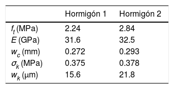
Experimental resultsTo validate the method for the determination of the softening curve, an experimental program of concrete fracture conducted by one of the authors was taken from the literature [13,15,16]. The experimental program encloses two ordinary concretes with design resistances 25 and 40MPa respectively.
In each one of the concretes, three compression tests, three Brazilian tests and six three point bending tests were carried out. In these last ones, 500×100×100mm beams with a depth of notch of 33mm were employed. The details of the experimental device can be found in [13,15,16]. The load-displacement obtained registers of opening at the end of the notch, P-CMOD are shown in Figs. 1 and 2.


The tests were stable up to the end. In all the cases is possible to observe a first step approximately lineal followed by a drop of load up to reach values close to zero. This drop of load was produced by the stable propagation of the crack along the symmetry plane of the sample (Fig. 3 and Table 1).
Numerical simulation
The three point bending tests were simulated by using the finite element model with the commercial code ABAQUS v6.9.3. The simulation was performed in two dimensions for adopting the hypothesis of plane stress. The mesh employed is formed by quadratic elements with four nodes and 400 elements in the ligament of the sample.
In the ligament of the mesh a band of non-lineal springs was introduced. Its behavior is ruled by the softening curve. In a first calculus a bilinear curve was considered, obtaining the following figures.
The numerical results were compared with the average curve of the experimental results. A good adjustment between the experimental and numerical data can be observed, but however, none of them can be considered as perfect.
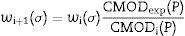
Iterative algorithm AMS-UPMTo improve the adjustment of Figs. 4 and 5, a modification of the softening curve is proposed. In this way, two successive transformations were conducted. The first one is applied to the cohesive displacement, w, defining a new softening curve σi+1=f(wi+1) calculated as:


The cohesive stress, σ, and the applied load, P are linked by the following expression:
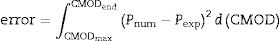
where β is an adimensional coefficient, between 0.5 and 3 (0.5, 1.0, 1.5, 2.0, 2.5 and 3), and Pmax is the maximum load. Each β value gives a different softening curve and a corresponding calculation. The next figures show the transformation 1 of the process of the iterative calculus. Fig. 6 compares the experimental curve (continuous curve) with the numerical corresponding to iteration i (curve of points). With Eqs. (1) and (2) six new softening curves are obtained (Fig. 7). β value leads to a minimum quadratic errorwhere Pnum is the numerical load, Pexp the experimental one, CMODMax is the CMOD under the maximum experimental load and CMODend is the value corresponding to the final load. This new softening curve does not produce a perfect adjustment of the experimental curve, but it improves the previous one (Fig. 8).


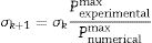
Applying successively the mentioned procedure, the softening curve is modified up to reach a softening curve where the application of Eq. (1) does not reduce the error. At this moment, the transformation 2 will be employed. This transformation consists in reducing the cohesive resistance proportionally to the numerical and experimental maximum load (4)
The modification type 2 is applied once and then is applied again the modification type 1.
The procedure finishes when the transformed softening curve by Eqs. (1) and (3) does not improve the adjustment of the experimental results. The numerical implementation of the proposed algorithm has been conducted by means of Python, the language employed by the finite element code ABAQUS to write the exit of results. In order to simplify the calculus procedure, a non-commercial application, BUCLE_TPB_H [17], has been developed. This application allows to develop calculus, to analyze results and modify the softening curve automatically.
ResultsThe previous algorithm has been applied to two conventional concretes described in the point 2, experimental results. In both cases, the softening curve which better adjust the average curve of the experimental results load-CMOD of the three point bending test has been obtained.
The next figures show the high quality of the adjustment obtained. In both cases, there is an excellent agreement between the numerical and experimental results (Figs. 9–10).


The final softening curves has been depicted in Fig. 11 and in Fig. 12, where they are compared with the initial bilinear curves. In both cases, the final curve maintains, approximately, the initial slope of the bilinear curve, softening the zone close to the point of intersection of the both lines of the bilinear curve.
Conclusions

In this paper, an original iterative method to determine the softening curve in concrete is proposed. This procedure reduces the different between the numerical and the experimental results modifying successively the softening curve. This algorithm has been successfully applied to two conventional concretes.
The softening curve obtained as a result of the application of the algorithm adjusts in a perfect way the average curve load-CMOD of three point bending tests.
The final softening curve does not suppose a remarkable modification of the bilinear softening curve. The current work does not propose a method alternative to the one based on a bilinear softening curve, it proposes a complementary procedure to improve the adjustment between the numerical and the experimental data.