Determination of minor and trace elements in geological materials used as raw ceramic materials

Abstract

A study has been undertaken to develop a methodology to determine minor and trace elements in geological ceramic raw materials by wavelength-dispersive X-ray fluorescence (WD-XRF) spectrometry. The set up of the methodology has been done either by optimising not only the sample preparation process but also optimising the measurement with the aid of the software Pro-Trace, and also by making an exhaustive compilation of reference materials for calibration and validation.

The developed method is precise and accurate and allows the analysis of Ba, Ce, Co, Cr, Cu, Fe, La, Mn, Ni, Pb, Rb, S, Sr, Ta, Th, U, V, Y, Zn and Zr present in the sample as minor or trace elements in geological materials used as raw ceramic material in a relatively short period of time. Besides, the method is more environmentally friendly than other methodologies as it does not require the use of solvents or reagents.

Resumen

Se ha llevado a cabo un estudio para el desarrollo de una metodología para la determinación de elementos minoritarios y traza en materias primas geológicas cerámicas mediante espectrometría de fluorescencia de rayos X por dispersión de longitudes de onda (WD-FRX). La puesta en marcha se ha llevado a cabo no solo mediante la optimización del proceso de preparación de muestra sino mediante la optimización de la medida con la ayuda del software Pro-Trace y mediante una exhaustiva recopilación de materiales de referencia para calibración y validación.

El método desarrollado es preciso y exacto, y permite el análisis de Ba, Ce, Co, Cr, Cu, Fe, La, Mn, Ni, Pb, Rb, S, Sr, Ta, Th, U, V, Y, Zn y Zr presentes en la muestra como elementos minoritarios y traza en materiales geológicos utilizados como materias primas cerámicas en un tiempo relativamente corto. Además, el método es más respetuoso con el medio ambiente que otras metodologías ya que no requiere el uso de disolventes o reactivos.

Introduction

The development of new analysis methods capable of determining minor and trace elements in ceramic raw materials has been demanded because of the emergence of new ceramic products with technical characteristics and novel functionalities demands, as some elements present in very low concentrations can generate defects in the final product.

The presence of compounds such as pyrites and other sulfur compounds that can decompose at elevated temperatures during the firing process of ceramic materials originates defects in the final product; other elements such as Ti and Fe compounds generate colouring problems, and the presence of U and Th in materials such as zirconium silicates can cause high levels of radioactivity.

Trace elements in rocks have often been determined using atomic absorption spectrometry (GFAAS or FIAS-AAS), inductively coupled plasma atomic emission spectrometry (ICP-OES) and inductively coupled plasma mass spectrometry (ICP-MS), which are extremely sensitive but require a tedious pretreatment, including decomposition with acid, due which implies the conduction of digestions, entailing the ensuing increase of the uncertainty and long analysis times, for that reason, analyses of numerous samples are difficult by these methods [1]. Bennett, in his book “XRF analysis of ceramics, minerals, and allied materials” [2], gives a general idea of how to characterise ceramics, minerals, and allied materials by WD-XRF, but does not refer to the analysis of trace elements.

The use of XRF in the analysis of geological samples is increasing, mainly because of the precision and accuracy with which the major elements and a wide range of trace elements may be determined. Although it is an old and well-established technique, it continues to find widespread use in the analysis of soils and other environmental samples. One reason for the continuing popularity of the technique is the simple sample preparation [3]. Its contribution to a substantial extent to the complete elemental characterisation allows the elucidation of its geological origin or the study of the evolution of mineral deposition with time. Furthermore, XRF is frequently used for the verification of the quality and the physical characteristics of industrial mineral processes. Across the years, many authors have pointed out the new applications of XRF in the field of geological minerals [4,5]. In the field of nanotechnology and the development of catalysts and new ceramic materials, the XRF technique continues to be one of the favourable analytical tools routinely applied in the characterisation process of these materials [6,7]. Another advantage of XRF against classical techniques is the analysis of U and Th, present in geological samples in very low concentrations. Techniques such as spectrophotometry, spectrofluorimetry, flame and graphite furnace AAS, ICP-OES, or neutron activation analysis (NAA) present different interferences and/or low sensitive which increase their detection limit of U and Th, which entail the necessity of a tedious sample preparation to concentrate these analytes [8].

This study has been undertaken to obtain such a methodology for the determination of minor and trace elements in materials such as sands, clays, kaolins, feldspars and feldspathoids, calcites, dolomites, etc., by wavelength dispersive X-ray fluorescence spectrometry (WD-XRF), and making an exhaustive compilation of reference materials to calibrate and validate the methodology. The following elements were analysed: Ba, Ce, Co, Cr, Cu, Fe, La, Mn, Ni, Pb, Rb, S, Sr, Ta, Th, U, V, Y, Zn y Zr.

The developed method is precise and accurate and allows the analysis of minor and trace elements in geological materials used as raw ceramic material in a relatively short period of time. The use of a great number of standards has yield a huge concentration range for all the analysed elements. Besides, the method is more environmentally friendly than other methodologies as it does not require the use of solvents or reagents due to the lack of any sample digestion process; reducing in this way the adverse environmental impact of analytical methodologies [9].

Experimental

Materials and equipment

The importance of “reliable” analyses of rocks reference materials in the calibration of modern instrumental techniques has already been stressed. In this respect, compilations of data for all available silicate samples are very valuable. However, these lists of data do have one drawback: they give little indication of the error limits in quoted values apart from a crude classification into “usable”, “proposed”, or “recommended” values as opposed to “for information” or “order of magnitudes values” depending on the favoured terminology of the compiler. The calculation of statistically meaningful uncertainty limits from such data is not simple since interlaboratory bias cannot readily be quantified on a statistical basis [10].

The results of many geological reference materials indicate that there are few major elements whose values are known with a confidence better than 1% (one sigma). Furthermore, for several elements, coefficients of variation exceed 5%, sometimes substantially so, even though the concentration of the element is significantly above the expected detection limit of modern analytical techniques. And so we have the contradiction that many modern instrumental methods are capable of achieving instrument precisions often exceeding 0.1% relative. Uncertainties in analyses of individual reference materials used for calibrating instruments can be overcome by incorporating a large number of such samples (often over 20) in the calibration data set do that discrepancies will cancel out. However, the only way in which the accuracy of a calibration can be satisfactory tested is by the analysis of individual reference and comparing analysed results with data [10].

In the case of trace elements, with a few notable exceptions, error in the analyses of reference materials usually exceeds 5% relative (one sigma). The problems mentioned for setting up and assessing the accuracy of major element calibrations are even more serious for trace element data. An associated difficulty is that is often necessary to determine these elements down to detection limit levels. Such data cannot be achieved unless the calibration line passes through the origin, and in instruments that are calibrated directly from reference materials, this is not always easy to achieve without a highly critical evaluation of the reliability of individual datum points [10].

The preparation of the calibration curves and validation of the measurements were carried out with materials coming from different origins:

• •

  Reference materials from different certification bodies:

  • -

    National Research Centre for Certified Reference Materials GBW (China): GBW07401 Soil, GBW07402 Soil, GBW07403 Soil, GBW07404 Soil, GBW07405 Soil, GBW07406 Soil, GBW07407 Soil, GBW07408 Soil, GBW03122 Kaolin, GBW07152 Lithium Ore, and GBW07153 Lithium Ore.

  • -

    Bureau of Analysed Samples – BAS (United Kingdom): BCS-CRM No. 313/1 High Purity Silica, and BCS-CRM No. 3751/1 Soda Feldspar.

  • -

    Canadian Centre for Mineral and Energy Technology – CANMET (Canada): STDS-1 Stream sediment, STDS-2 Stream sediment, STDS-3 Stream sediment, STDS-4 Stream sediment, SY-2 Syenite, and SY-3 Syenite.

  • -

    Instituto de Pesquisas Tecnologicas (Brazil): IPT-72 Soda Feldspar.

• •

  Reference materials obtained from the participation in round robin test organised by different associations:

  • -

    GeoPT series of reference materials obtained from the Interlaboratory Test for the Analysis of geological samples (GeoPT) organised by IAG (International Association of Geoanalysts) (United Kingdom): GeoPT-7 Biotite, GeoPT-8 Microdiorite, GeoPT-11 Dolerite, GeoPT-12 Serpentinite, GeoPT-16 Basalt rock, GeoPT-19 Gabbro, GeoPT-20 Ultramafic rock, GeoPT-21 Granite, GeoPT-22 Basalt, GeoPT-23 Lake pegmatite, GeoPT-24 Greywake, GeoPT-25 Basalt, GeoPT-28 Shale, GeoPT-29 Nepheline, GeoPT-30 Syenite, GeoPT-30A Limestone, GeoPT-31 River sediment, GeoPT-34 Basalt, GeoPT-35 Ball clay, and GeoPT-35A Metalliferous sediment.

  • -

    Mercury Soil-2 MS-2 obtained from the interlaboratory organised by the Central Geological Laboratory of Mongolia (CGL) (Mongolia).

Depending on the certification body and certification procedure, data with different quality can be found in the reference materials certificate, such as certified values with assigned uncertainty (combined (u) or expanded (U)), and reference values or information values with no uncertainty. Regarding the reference materials obtained from the participation in the Interlaboratory Test for the Analysis of geological samples (GeoPT) organised by IAG, we can find two types of materials:

• (a)

  Most of them present an assigned value (X_a) together with a parameter called target standard deviation (H_a), which is calculated from a modified form of the Horwitz function as follows:

  
  where X_a is the assigned value expressed as a fraction, and the factor k gets the value 0.01 or 0.02 depending on the kind of laboratory that gave the individual result (for example, “pure geochemistry labs”, which are those which analytical results are designed for geochemical research and care is taken to provide data of high precision and accuracy; or “applied geochemistry labs”, which main objective is to provide results on large number of samples collected).

• (b)

  A few of them are submitted to a subsequent certification process (GeoPT-16, GeoPT-14, and GeoPT-12) and some elements present an assigned value (X_a) accompanied by its uncertainty (U).

As can be seen from the relation of reference materials used in this study, materials of different nature and with a variety of matrix were used in the preparation of the calibration curves. After the calibration was performed, geological materials different from those used in the calibration were analysed and the results compared in other to validate the established methodology.

The study was conducted with a PANalytical model AXIOS wavelength dispersive X-ray fluorescence (WD-XRF) spectrometer with a Rh anode tube, and 4 kW power, fitted with flow, scintillation, and sealed detectors, eight analyzing crystals: LiF200, LIF220, Ge, TLAP, InSb, PE, PX1 and PX7, and provided with masks of 37, 30, 27, 10, and 6 mm in diameter.

Optimisation of the sample preparation

Although XRF analysis requires only simple preparation techniques, sample preparation is usually necessary to ensure XRF analysis to be truly effective and contribute to the optimisation of X-ray analysis [11]. This sample preparation is much less time consuming than that necessary in other analytical techniques such as ICP-OES, ICP-MS, GFAAS or FIAS-AAS, requiring sample preparation times over 10 min versus several hours for the analysis by these last mentioned techniques.

For WD-XRF analysis, the sample needs to be prepared in the form of pellets or beads. When the analyte is present in the sample in very low concentration (minor or trace), the sample is prepared in the form of pressed pellets in order to have lower detection limits as the sample does not suffer any significant dilution during the sample preparation.

There is literature where the analysis of rare earth elements in rocks by WD-XRF was carried out preparing the sample as beads with a very low dilution which obliged them to reheat the glass at 1200 °C with its consequent loss of volatile analyte and increase of uncertainty due to the higher manipulation of the sample [1].

The pellet preparation was optimised forming pellets of a soil with different binders and studying the one that gave the best results, that is, better surface, and better reproducibility in the results. Four binders were studied: d-mannitol, stearic acid, n-butyl methacrylate and a mixture of polyvinylpyrrolidone (PVP) and methyl cellulose (MC). Table 1 shows the pellet preparation for each binder used.

Table 1.

Pellet preparation conditions for each binder studied.

Binder	Binder preparation	Pellet preparation
d-Mannitol	–	10,000 g sample with 2000 g binder, mixed in a tungsten carbide mill for 40 s
Stearic acid	–
n-Butyl methacrylate	13.7% solution of n-butyl methacrylate in acetone	10,000 mg sample with 2.5 ml of the solution, mixed manually in an agate mortar
Polivinylpyrrolidone and methyl cellulose (PVP-MC)	40 g of MC dissolved in 400 ml deionised boiled water mixed with a solution of 70 g PVP in 300 ml ethanol	10,000 g sample with 2 drops of the PVP-CM solution per gram, mixed manually in an agate mortar
		After forming the pellet, dried in an oven at 110 °C for a minimum of 10 min to get the process of binding formed

All pellets were formed at a pressure of 100 kN [11] in a CASMON hydraulic press using a 40-mm diameter die (being this the highest size for which a mask is available in the WD-XRF instrument).

After forming the pellets, their surface was observed, the one with stearic acid being the best. To confirm this, ten pellets were prepared using this binder and measured; the results obtained showing dispersion lower than 5% (relative). So, all pellets were prepared using stearic acid as binder.

As can be seen in Table 1, the sample and stearic acid are mixed in a tungsten carbide ring mill for 40 s. Tungsten carbide presents cobalt in its composition, which is one of the analytes of interest. So, to assure that no contamination occurred during sample preparation, the mixture with the binder for pellet preparation was also carried out in an agate ring mill. Cobalt was then analysed in this pellet and the results compared with the pellet prepared in tungsten carbide ring mill, not having any significant difference between both preparations.

Calibration

Empirical calibration curves comparing intensities with concentrations can be used for the analysis of samples with limited variations of the matrix composition. However, a general-purpose calibration procedure that is applicable to a larger variety of matrix types and covering wider ranges of the analyte concentration is usually more desirable. The calibration procedure known as “empirical” compares directly the net intensity of the analyte peaks with their concentrations, without making any correction for the inter-element of matrix effects. It is possible to use this type of calibration only when the analyte concentration range is limited and when the standard and sample matrix compositions are extremely similar. This can occur in certain industrial applications where the standards are normally typical “samples” that have been analysed by a technique other than XRF. With this calibration type, it is assumed that the net intensity is linearly related to concentration. However, the relationship between intensity and concentration becomes non-linear when significant differences in matrix compositions are present between samples and standards. The analyst must be extremely cautious when using empirical coefficients calculated by multiple regression analysis because such an approach contains many potentials pitfalls. Not only do empirical coefficients correct for matrix effects, but they can also conceal other error types that may be present, such as errors on measured intensities, poor standard chemical data, poor sample preparation, variation of particle size effects, of mineralogical effects, of surface effects, and so on. As opposed to empirical coefficients, theoretically determined influence coefficients allow the error sources to be detected, isolated and estimated, thereby giving the analyst greater confidence in the reliability and applicability of the calibration data. When calibrating for an analyte, it must always be kept in mind that a significant intercept value means an error somewhere, and one must try to discover the cause of it and correct for it. In the case of trace element determination, the best method to correct the matrix effects lies in the use of theoretical influence coefficients, calibration curves should be constrained to pass through the origin, and, whenever possible, the use of linear regression analysis is recommended [12,13].

The measurement was undertaken with the aid of an analytical programme called Pro-Trace, supplied by PANalytical, which uses primary and secondary or only secondary mass attenuation coefficients (MAC's) to make matrix corrections or net intensities. Advantages of the use of Pro-Trace are: the more accurate background interpolation, the matrix effect correction thanks to MAC's and finally the smart element selector (SES) which allows the reduction of measurement times with the use of shared background positions [14]. Table 2 shows the measurement conditions.

Table 2.

Measurement conditions by WD-XRF.

Element	Line	Crystal	Detector	Voltage (kV)	Intensity (mA)	Angle (2θ) (°)	Bg1	Bg2	PHD LL	PHD UL	t (s)
Ba	Lα	LiF 200	Flow	40	90	87.1906	1.4048		30	60	60
Ce	Lβ1	LiF 220	Duplex^a	50	72	111.6862	−1.5356		30	60	60
Co	Kα	LiF 220	Duplex^a	60	60	77.891	1.4262		20	60	60
Cr	Kα	LiF 220	Duplex^a	50	72	107.1524	−1.2458	3.0002	30	60	60
Cu	Kα	LiF 220	Duplex^a	60	60	65.5376	−3.9523	2.7897	20	60	60
Fe	Kα	LiF 200	Duplex^a	60	60	57.4862			15	72	60
La	Kα	LiF 200	Flow	50	72	82.908	−0.7432		30	60	60
Mn	Kα	LiF 220	Duplex^a	60	60	95.2112	−2.2636	3.1564	15	60	60
Ni	Kα	LiF 220	Duplex^a	60	60	71.238	−2.9334	2.0164	20	60	60
Pb	Lβ1	LiF 220	Scintillation	60	60	40.3696		1.8335	35	65	60
Rb	Kα	LiF 220	Scintillation	60	60	37.9316			36	65	50
S	Kα	Ge 111	Flow	36	100	110.698	−1.9198	4.9502	30	65	50
Sr	Kα	LiF 220	Scintillation	60	60	35.8026	−0.9786	0.8565	35	65	40
Ta	Lα	LiF 220	Duplex^a	60	60	64.614			20	60	60
Th	Lβ1	LiF 220	Scintillation	60	60	37.2914			35	65	60
U	Lα	LiF 220	Scintillation	60	60	31.1626			35	65	60
V	Kα	LiF 220	Duplex^a	50	72	123.1798	3.0796		30	60	60
Y	Kα	LiF 220	Scintillation	60	60	33.844			35	65	40
Zn	Kα	LiF 220	Scintillation	60	60	60.55	−1.3669	1.0536	30	70	60
Zr	Kα	LiF 220	Scintillation	60	60	32.0462	0.7761		35	65	40

a

Sealed + Flow.

Once the calibration conditions were selected, the reference materials were measured in order to construct the calibration curves. Tables 3–6 show the concentrations of each element analysed for each of the calibration standards (X_a, for values obtained from interlaboratory results, or C_cert, for values obtained from a certificate of analysis), together with its uncertainty (U) or its target standard deviation (H_a) (when coming from a proficiency test).

Table 3.

Reference materials for calibration from GeoPT (GeoPT-7 to GeoPT-24).

Element (mg kg^−1)	GeoPT-7		GeoPT-8		GeoPT-11		GeoPT-12		GeoPT-16		GeoPT-19
	Xa	H	Xa	H	Xa	H	Xa	U^c	Xa	U^d	Xa	H
Ba	908	26.1	360.8	11.9	309.2	10.4	8.4^a	0.6	200^a	–	53.46	2.349
Ce	103.2	4.1	55.7	2.4	44.17	2	0.279	H-0.027	13.3^a	–	3.42	0.227
Co	19.5	1	13.5	0.73	38.6	1.78	106^b	3	49.7^a	–	35.34	1.653
Cr	181.4	6.6	54.7	2.4	38.4	1.77	2780^b	33	332^b	9	39.77^a	1.827
Cu	30	1.4	27.3	1.3	27.3	1.33	–	–	96^a	–	593.95	18.168
Fe (%)	4.21	0.09	4.07	0.06	10.21	0.14	5.59^b	0.15	7.24^b	0.03	7.52	0.11
La	52.95	2.33	24.96	1.23	18.1	0.94	0.15^a	0.016	5.2	H-0.32	1.38	0.105
Mn	542	20	1084	31	2401	54	635^b	70	1294^b	15	775	23
Ni	59.6	2.6	21	1.06	15	0.8	2296^b	120	150^a	–	19.65	1.004
Pb	14.1	0.76	14.1	0.76	4.66	0.3	–	–	3.3^b	0.2	4.55^a	0.29
Rb	56.24	2.45	98.5	3.9	19.29	0.99	–	–	1.91^b	0.01	–	–
S	–	–	–	–	–	–	–	–	–	–	–	–
Sr	363.5	12	99.9	4	226.8	8	7.34^b	0.35	169.2^b	0.7	786.94	23.073
Ta	0.4	0.04	1	0.08	0.546^a	0.048	–	–	0.28	H-0.03	–	–
Th	11.23	0.62	8.42	0.49	2.25	0.159	0.03^b	–	0.33^b	0.03	–	–
U	0.9	0.07	2.19	0.16	0.5	0.044	0.831^b	0.068	0.29^b	0.03	0.03	0.004
V	96.5	3.9	82.7	3.4	447.8	14.3	33.4^b	2	250^a	–	452.8	14.428
Y	18	0.93	47.1	2.1	51.8	2.3	–	–	19.33	H-0.99	4.44	0.284
Zn	80.3	3.3	69.5	2.9	133.6	5.1	38.6^b	3.2	58.0^b	–	93.3	3.771
Zr	231.8	8.2	195.1	7.1	219.9	7.8	–	–	55.1	H-2.4	10.00^a	0.566

Element (mg kg^−1)	GeoPT-20		GeoPT-21		GeoPT-22		GeoPT-23		GeoPT-24
	Xa	H	Xa	H	Xa	H	Xa	H	Xa	H
Ba	–	–	344.08	11.426	755.01	41.44	8.75^a	0.505	311	10.486
Ce	1.33	0.102	63.06	2.703	103.76	5.97	7.24^a	0.43	38^a	1.758
Co	86.46	3.534	2.73	0.188	25.65	3.81	–	–	12	0.661
Cr	2420.7	59.93	186.7	6.797	214.81	21.72	–	–	34	1.6
Cu	43.65	1.978	7	0.418	32.19	3.71	–	–	22.3	1.118
Fe (%)	8.28	0.11	1.69	0.029	6.84	0.15	0.52	0.01	3.44	0.05
La	0.42	0.038	29.22	1.407	55.88	3.39	2.03^a	0.146	18.8	0.967
Mn	1394	39	465	15	1007	39	852	23	929	23
Ni	870.62	25.141	5.92	0.362	159.3	12.5	–	–	17.7	0.919
Pb	–	–	25.42	1.249	8.59	1.94	–	–	26.9	1.309
Rb	1.04	0.082	271.94	9.356	62.89	3	2501	61.5	35.9	1.676
S	–	–	–	–	–	–	–	–	–	–
Sr	15.99	0.843	110.75	4.362	920.52	39.92	–	–	174	6.394
Ta	0.03^a	0.004	2.53	0.176	3.08	0.31	124.7^a	4.83	0.56	0.049
Th	0.03	0.004	19.19	0.984	6.84	1.34	5.08	0.318	5	0.316
U	0.01	0.002	5.43	0.337	1.67	0.42	4.37	0.28	1.09	0.086
V	167.85	6.281	14.01	0.753	105.03	7.57	–	–	77	3.209
Y	9.44	0.538	24.67	1.218	20.41	1.89	8.14^a	0.475	20.5	1.039
Zn	61.81	2.658	54.56	2.391	115.47	8.97	28.15	1.362	54	2.382
Zr	16.85	0.881	168.41	6.227	288	17.38	–	–	123	4.768

a

Data in italics is either provisional or informative.

b

Data in bold are certified values due to a subsequent certification process of the material.

c

U is the expanded uncertainty corresponding to a level of confidence of 95%.

d

U based on judgement and represents an evaluation of the combined effects of method imprecision, possible systematic errors among methods and material variability.

Table 4.

Reference materials for calibration from GeoPT (GeoPT-25 to GeoPT-35A).

Element (mg kg^−1)	GeoPT-25		GeoPT-26		GeoPT-28		GeoPT-29		GeoPT-30
	Xa	U^c	Xa	H	Xa	H	Xa	H	Xa	H
Ba	555^b	7	512	16.002	788^a	23.099	741^a	27.85	684.1	20.485
Ce	93.3^b	1.2	48.9	2.178	108.2	4.276	124.3^a	2.74	252.4	8.781
Co	37.5^b	1.4	21.4	1.079	22.7	1.135	63.7	–	2.75^a	0.189
Cr	12.4^b	1	–		109	4.303	438	–	18^a	0.932
Cu	160^b	3	23.7^a	1.179	31.2	1.487	56.5	–	–	–
Fe (%)	10.90^b	0.06	2.23	0.01	6.79	0.017	9.29^a	0.098	2.82	0.009
La	42.6^b	1	25.9	1.271	52.5	2.312	62.6	1.801	145.3	5.493
Mn	1496^b	21	3129	23	1162	8	1572	178	1239	7
Ni	22.1	H-0.364	87.0^a	3.552	82.8	3.408	315	–	77.8	3.232
Pb	5.44	H-0.089	7.2^a	0.426	35	1.639	2.88^a	–	15.95	0.841
Rb	35.4	H-0.285	14.7	0.783	147	5.548	31.4	7.97	248.9	8.678
S	–	–	–	–	–	–	–	–	–	–
Sr	481.8	H-2.874	118.2	4.61	178	6.527	1175	1032	302.7	10.248
Ta	1.93	H-0.027	0.35^a	0.033	1.11	0.087	5.14^a	0.074	6.62	0.398
Th	3.98	H-0.259	3.93	0.256	15.8	0.836	7.4	0.318	32.28	1.531
U	0.81	H-0.067	0.83	0.068	5.76	0.354	2.2	1.15	8.4	0.488
V	392.8	H-2.613	64.0^a	2.736	220	7.814	292^a	3.17	23	1.148
Y	39.93	H-0.466	15.5	0.822	36.5	1.697	29.5	2.11	40	1.836
Zn	141.5	H-1.496	27.8^a	1.349	186.8	6.8	117.4	–	61.6	2.651
Zr	310.1	H-1.816	81.2	3.352	134.3	5.137	292	–	838.5	24.351

Element (mg kg^−1)	GeoPT-30A		GeoPT-31		GeoPT-34		GeoPT-35		GeoPT-35A
	Xa	H	Xa	H	Xa	H	Xa	U	Xa	H
Ba	27.85^a	1.35	733	733	865.9	49.69	733	21.72	865.9	25.02
Ce	2.74^a	0.188	28.3	28.3	89.32	6.181	28.3	1.368	89.32	3.634
Co	–	–	19.34	19.34	55.59	0.2919	19.34	0.9904	55.59	2.429
Cr	–	–	–	–	–	0.977	–	–	–	–
Cu	–	–	20	20	1159	0.8142	20	1.019	1159	32.06
Fe (%)	0.098^a	0.001	5.27	5.27	4.51	0.03	5.27	0.08	4.51	0.013
La	1.801	0.132	12.56	12.56	44.89	3.7564	12.56	0.6865	44.89	2.025
Mn	178	4	894.7	894.7	3989	9	894.7	25	3989	88
Ni	–	–	6^a	6	230	0.4214	6^a	0.3665	230	8.115
Pb	–	–	14	14	3893	1.4767	14	0.7527	3893	89.73
Rb	7.97	0.467	60.75	60.75	152.3	6.201	60.75	2.619	152.3	5.716
S	–	–	–	–	–	–	–	–	–	–
Sr	1032	29.04	294.1	294.1	182.2	14.777	294.1	9.999	182.2	6.657
Ta	0.074^a	0.009	0.401	0.401	1.41	0.0773	0.401	0.037	1.41	0.1071
Th	0.318	0.03	3.92	3.92	17.74	1.2084	3.92	0.2553	17.74	0.9204
U	1.15	0.09	1.274	1.274	4.068	0.1528	1.274	0.09828	4.068	0.2634
V	3.17^a	0.213	145.7	145.7	73.15	1.6688	145.7	5.506	73.15	3.067
Y	2.11	0.151	23.95	23.95	25.41	0.5553	23.95	1.188	25.41	1.249
Zn	–	–	89.94	89.94	3684	3.5532	89.94	3.651	3684	85.61
Zr	–	–	125.5	125.5	257.9^a	11.041	125.5	4.851	257.9^a	8.942

a

Data in italics is either provisional or informative.

b

Data in bold are certified values due to a subsequent certification process of the material.

c

U is the expanded uncertainty for 95% confidence and contains a contribution from the characterisation of the laboratory and a contribution from the material heterogeneity

Table 5.

Reference materials for calibration from BAS, CANMET, IPT, and CGL.

Element (mg kg^−1)	MS-2		BCS-CRM No. 313/1		IPT-72		SY-2		SY-3		STSD-1		STSD-2		STSD-3		STSD-4		BCS-CRM No. 375/1
	Xa	U	Ccert	s^b	Xa	U^c	Cknown	U	Cknown	U	Cknown	U	Cknown	U	Cknown	U	Cknown	U	Ccert	U^c
Ba	–	–	–	–	–	–	460^a	–	430^a	–	630^a	–	540^a	–	1490^a	–	2000^a	–	95	–
Ce	–	–	–	–	–	–	210^a	–	2200^a	–	51^a	–	93^a	–	63^a	–	44^a	–	54	–
Co	–	–	–	–	–	–	11^a	–	12^a	–	17^a	–	19^a	–	16^a	–	13^a	–	–	–
Cr	–	–	–	–	–	–	12^a	–	10^a	–	67^a	–	116^a	–	80^a	–	93^a	–	12	–
Cu	–	–	–	–	–	–	5^a	–	16^a	–	36^a	–	47^a	–	39^a	–	65^a	–	–	–
Fe (%)	2.95^a	–	0.008	0.0006	0.063	0.01	4.39^a	–	4.49^a	–	4.54^a	–	5.24^a	–	4.33^a	–	3.99^a	–	0.203	0.008
La	–	–	–	–	–	–	88^a	–	1350^a	–	30^a	–	59^a	–	39^a	–	24^a	–	26	–
Mn	–	–	1.3	0.3	–	–	2479^a	–	2479^a	–	0.38^a	–	775^a	–	2324^a	–	1550^a	–	–	–
Ni	–	–	–	–	–	–	10^a	–	11^a	–	24^a	–	53^a	–	30^a	–	30^a	–	–	–
Pb	–	–	–	–	–	–	80^a	–	130^a	–	35^a	–	66^a	–	40^a	–	16^a	–	4	–
Rb	–	–	–	–	–	–	220^a	–	208^a	–	30^a	–	104^a	–	68^a	–	39^a	–	52	–
S	930^a	–	–	–	–	–	110^a	–	500^a	–	1800^a	–	600^a	–	1400^a	–	900^a	–	–	–
Sr	–	–	–	–	–	–	275^a	–	306^a	–	170^a	–	400^a	–	230^a	–	350^a	–	101	–
Ta	–	–	–	–	–	–	–	–	–	–	0.4^a	–	1.6^a	–	0.9^a	–	0.6^a	–	–	–
Th	–	–	–	–	–	–	380^a	–	990^a	–	3.7^a	–	17.2^a	–	8.5^a	–	4.3^a	–	10	–
U	–	–	–	–	–	–	290^a	–	650^a	–	8.0^a	–	18.6^a	–	10.5^a	–	3.0^a	–	2	–
V	–	–	–	–	–	–	52^a	–	51^a	–	98^a	–	101^a	–	134^a	–	106^a	–	–	–
Y	–	–	–	–	–	–	130^a	–	740^a	–	42^a	–	37^a	–	36^a	–	24^a	–	18	–
Zn	–	–	–	–	–	–	250^a	–	240^a	–	178^a	–	246^a	–	204^a	–	107^a	–	4	–
Zr	–	–	–	–	–	–	280^a	–	320^a	–	218^a	–	185^a	–	196^a	–	190^a	–	79	–

a

Data in italics is either provisional or informative.

b

Standard deviation.

c

The uncertainty (U) has been calculated as U=tα⋅s/N, with where α = 0.05 (95% confidence), s is the standard deviation, and N is the number of acceptable data.

Table 6.

Reference materials for calibration from the National Research Centre for Certified Reference Materials GBW.

Element (mg kg^−1)	GBW 07401		GBW 07402		GBW 07403		GBW 07404		GBW 07405		GBW 07406		GBW 07408		GBW 03122		GBW 07152
	Ccert	U^b	Ccert	U^b	Ccert	U^b	Ccert	U^b	Ccert	U^b	Ccert	U^b	Ccert	U^b	Ccert	S^a	Ccert	s^a
Ba	590	15	930	24	1210	30	213	10	296	12	118	6	480	11	–	–	–	–
Ce	70	2	402	10	39	2	136	6	91	6	66	3	66	4	–	–	7.3	0.6
Co	14.2	0.4	8.7	0.3	5.5	0.2	22	0.6	12	0.5	7.6	0.4	12.7	0.4	–	–	–	–
Cr	62	2	47	2	32	2	370	6	118	3	75	2	68	2	–	–	–	–
Cu	21	0.6	16.3	0.4	11.4	0.4	40.5	0.1	144	3	390	6	24.3	0.5	–	–	–	–
Fe (%)	3.63	0.03	2.46	0.02	1.4	0.01	7.2	0.03	8.83	0.05	5.66	0.04	3.13	0.01	0.56	0.03	0.275	0.013
La	34	1	164	5	21	1	53	2	35.7	1.8	30	1	35.5	1.4	–	–	4.3	0.2
Mn	1760	24	510	6	304	5	1420	30	1360	28	1450	32	650	9	54	11	540	40
Ni	20.4	0.6	19.4	0.5	12.2	0.4	64.2	1.7	40	1	53	1	31.5	0.7	–	–	–	–
Pb	98	3	20.2	1	26	2	58.5	2.1	552	14	314	6	21	1	–	–	–	–
Rb	140	3	88	2	85	2	75	2	117	3	237	4	96	2	–	–	0.13%	0.01%
S	310	60	210	30	120	10	180	30	410	40	260	30	120	30	480	40	–	–
Sr	155	3	187	4	380	8	77	3	41.5	1.9	39	2	236	6	–	–	–	–
Ta	1.4	0.1	(0.8)^c	–	(0.8)^c	–	3.1	0.2	1.8	0.2	5.3	0.4	1.05	0.16	–	–	40.5	3.8
Th	11.6	0.7	16.6	0.8	6	0.5	27	2	23	2	23	2	11.8	0.7	–	–	–	–
U	3.3	0.4	1.4	0.3	1.3	0.3	6.7	0.8	6.5	0.7	6.7	0.7	2.7	0.4	–	–	–	–
V	86	2	62	2	36.5	1.1	247	6	166	4	130	3	81.4	1.8	–	–	–	–
Y	25	1	21.7	0.9	15	1	39	2	21	1	18.8	0.8	26	1	–	–	13.3	1.4
Zn	680	11	42.3	1.2	31.4	1.1	210	5	494	11	96.6	2.4	68	2	–	–	–	–
Zr	245	6	219	8	246	7	500	21	272	8	220	7	229	6	–	–	–	–

a

Standard deviation.

b

The uncertainty (U) has been calculated as U=tα⋅s/N, where α = 0.01 (99% confidence), s is the standard deviation, and N is the number of data (N > 8).

c

Data enclosed in brackets are reference values.

The software of the instrument permits the quality of the value to be defined. In this way, assigned values from GeoPT proficiency test and certified values were defined as high quality, while those provisional, reference or informative where defined as low quality. The software fits the experimental data taking into account the quality of each value, minimising the RMS value (root mean square), obtained from the following equation:

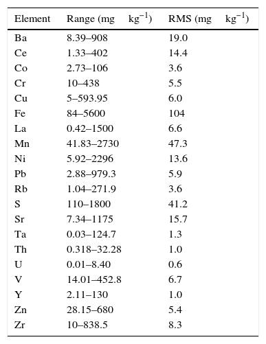
where C^* is the known mass fraction, C is the calculated mass fraction, n is the number of calibration standards, and p is the number of calculated regression parameters (slope, ordinate at the origin, and interelement coefficients). The definition of high and poor quality data permitted the improvement of the RMS obtained. Table 7 shows the results of RMS and the working range of all the elements analysed, studying the standards selected in each calibration curve from Tables 3–6 in order to obtain the required range for this study.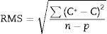

Table 7.

RMS value and working range in the measurement of each element analysed by WD-XRF.

Element	Range (mg kg^−1)	RMS (mg kg^−1)
Ba	8.39–908	19.0
Ce	1.33–402	14.4
Co	2.73–106	3.6
Cr	10–438	5.5
Cu	5–593.95	6.0
Fe	84–5600	104
La	0.42–1500	6.6
Mn	41.83–2730	47.3
Ni	5.92–2296	13.6
Pb	2.88–979.3	5.9
Rb	1.04–271.9	3.6
S	110–1800	41.2
Sr	7.34–1175	15.7
Ta	0.03–124.7	1.3
Th	0.318–32.28	1.0
U	0.01–8.40	0.6
V	14.01–452.8	6.7
Y	2.11–130	1.0
Zn	28.15–680	5.4
Zr	10–838.5	8.3

Very low RMS value was obtained for all the analysed elements, which depends on the number and quality of standards, the interelement coefficients calculated, the range and of course the quality of the measurement process.

Figs. 1–4 show the calibration curve obtained for four of the elements as an example. Data in green are the ones defined as high quality whereas data in red in the one defined as low quality (because they are reference or informative values).

Fig. 1.

Calibration curve for vanadium.

Fig. 2.

Calibration curve for nickel.

Fig. 3.

Calibration curve for cupper.

Fig. 4.

Calibration curve for manganese.

Validation

After the calibration was performed, the following reference materials were analysed by WD-XRF in order to validate the developed method: GeoPT-9 Slate, GBW07153 Lithium Ore, and GBW07407 Soil.

Calculation of the detection limit (L_D) and quantification limit (L_Q)

The L_D was calculated from the measurement of a sample with a concentration 0.5 times the concentration of the lowest standard in the calibration curve for each analyte. The sample was measured ten times under reproducibility conditions. The detection limit was obtained in accordance with the International Union of Pure and Applied Chemistry (IUPAC) guidelines from the following expression:

where s = value of the standard deviation of the measurements.

The L_Q, which expresses the quantifiability of an analyte, was calculated according to the IUPAC guidelines as ten times the standard deviation of the measurement, for a number of measurements equal to ten [15,16]:

Calculation of the measurement uncertainty

The measurement uncertainty [17] was calculated as U = ku_method, where u_method is the combined uncertainty calculated from the expression:

where uVR is the uncertainty of the certified value of the reference material, uVL is the uncertainty of the measurement of the reference material and uREPRO is the uncertainty of the measurement of the sample.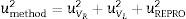

uVL and uREPRO were calculated from the expression s/n, where s is the standard deviation of the reference material measurement or the standard deviation of the sample measurement under reproducibility conditions, depending on the term calculated, and n is the number of measurements under reproducibility conditions. The coverage factor k is determined from the Student's t-distribution corresponding to the appropriate degrees of freedom and 95% confidence.

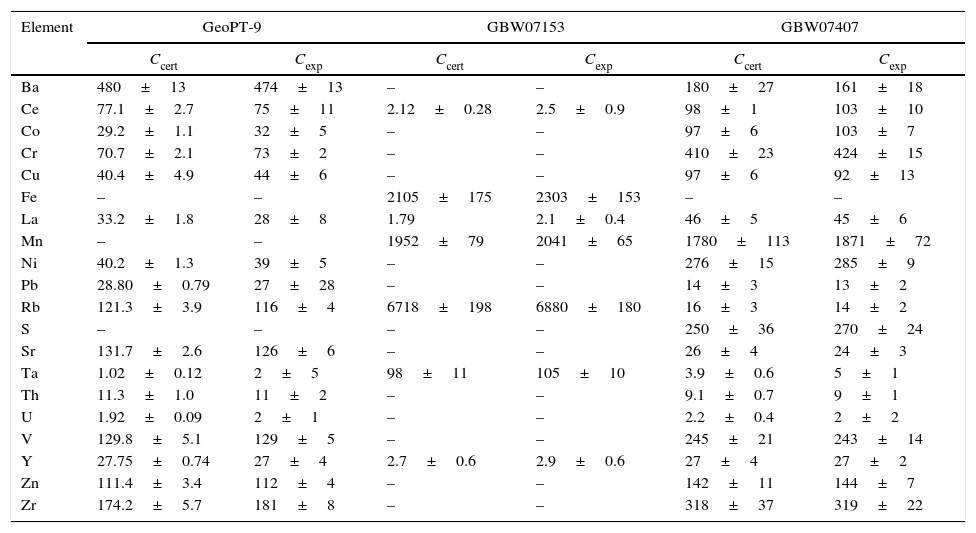
Results

Validation of the methodology

Once the calibrations were performed, the methodology was validated measuring reference materials. The results obtained, together with their uncertainty (U) calculated from expression [5], are presented in Table 8.

Table 8.

Validation of the calibration curves.

Element	GeoPT-9		GBW07153		GBW07407
	Ccert	Cexp	Ccert	Cexp	Ccert	Cexp
Ba	480 ± 13	474 ± 13	–	–	180 ± 27	161 ± 18
Ce	77.1 ± 2.7	75 ± 11	2.12 ± 0.28	2.5 ± 0.9	98 ± 1	103 ± 10
Co	29.2 ± 1.1	32 ± 5	–	–	97 ± 6	103 ± 7
Cr	70.7 ± 2.1	73 ± 2	–	–	410 ± 23	424 ± 15
Cu	40.4 ± 4.9	44 ± 6	–	–	97 ± 6	92 ± 13
Fe	–	–	2105 ± 175	2303 ± 153	–	–
La	33.2 ± 1.8	28 ± 8	1.79	2.1 ± 0.4	46 ± 5	45 ± 6
Mn	–	–	1952 ± 79	2041 ± 65	1780 ± 113	1871 ± 72
Ni	40.2 ± 1.3	39 ± 5	–	–	276 ± 15	285 ± 9
Pb	28.80 ± 0.79	27 ± 28	–	–	14 ± 3	13 ± 2
Rb	121.3 ± 3.9	116 ± 4	6718 ± 198	6880 ± 180	16 ± 3	14 ± 2
S	–	–	–	–	250 ± 36	270 ± 24
Sr	131.7 ± 2.6	126 ± 6	–	–	26 ± 4	24 ± 3
Ta	1.02 ± 0.12	2 ± 5	98 ± 11	105 ± 10	3.9 ± 0.6	5 ± 1
Th	11.3 ± 1.0	11 ± 2	–	–	9.1 ± 0.7	9 ± 1
U	1.92 ± 0.09	2 ± 1	–	–	2.2 ± 0.4	2 ± 2
V	129.8 ± 5.1	129 ± 5	–	–	245 ± 21	243 ± 14
Y	27.75 ± 0.74	27 ± 4	2.7 ± 0.6	2.9 ± 0.6	27 ± 4	27 ± 2
Zn	111.4 ± 3.4	112 ± 4	–	–	142 ± 11	144 ± 7
Zr	174.2 ± 5.7	181 ± 8	–	–	318 ± 37	319 ± 22

In order to compare the results obtained with the known values of the validation standards, the difference between both was compared, together with the related uncertainty: that is, the combined uncertainty of the known and measured values, as specified in the literature [18].

The absolute value of the difference between the measured value and the known value is calculated as follows:

where Δ_m = absolute value of the difference between the measured and the known value; c_m = measured value; c_known = known or certified value.

The uncertainty of Δ_m is calculated from the uncertainty of the known/certified value and the uncertainty of the measured value from the following formula:

where u_Δm = combined uncertainty of the result and of the known value; u_m = uncertainty of the measured value; u_known = uncertainty of the known value.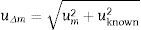

The expanded uncertainty U_Δm is obtained by multiplying u_Δm by a coverage factor (k), usually equal to two, which corresponds approximately to a 95% level of confidence. Thus:

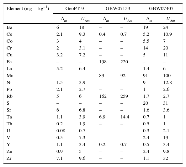
In order to verify the goodness of the method, Δ_m is compared with U_Δm, such that if Δ_m ≤ U_Δm, there is no significant difference between the measured value and the known value.

The results of this comparison are presented in Table 9. For the comparison of the results obtained in the measurement of the reference material named GBW07153, the uncertainty of the certified values was calculated from the standard deviation and number of data shown in the certificate with a level of confidence of 95%, in order to be able to apply the statistical test.

Table 9.

Comparison of the results of the WD-XRF measurements of the validation standards with the certified values.

Element (mg kg^−1)	GeoPT-9		GBW07153		GBW07407
	Δm	UΔm	Δm	UΔm	Δm	UΔm
Ba	6	18	–	–	19	24
Ce	2.1	9.3	0.4	0.7	5.2	10.9
Co	3	4	–	–	5.5	7
Cr	2	3.1	–	–	14	20
Cu	3.2	7.2	–	–	5	11
Fe	–	–	198	220	–	–
La	5.2	6.4	–	–	1.4	6
Mn	–	–	89	92	91	100
Ni	1.5	3.9	–	–	9	12.8
Pb	2.1	2.7	–	–	1	2.6
Rb	5	6	162	259	1.7	2.7
S	–	–	–	–	20	31
Sr	6	6.8	–	–	1.6	3.6
Ta	1.1	3.9	6.9	14.4	0.7	1
Th	0.2	1.9	–	–	0.5	1
U	0.08	0.7	–	–	0.3	2.1
V	0.5	7.3	–	–	2.4	19
Y	1.1	3.4	0.2	0.7	0.5	3.4
Zn	0.9	5	–	–	2.4	9.8
Zr	7.1	9.6	–	–	1.1	32

The value of Δ_m is smaller than U_Δm for all the elements analysed which indicates that there is not a significant difference between the results obtained and the certified value, making the developed methodology validated. Nor uncertainty or standard deviation was declared for lanthanum in GBW07153 reference material, so this comparison could not be made for this element, but comparing both the certified and measured value, no significant differences where found.

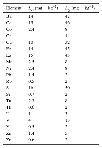
Calculation of the detection limit (L_D) and quantification limit (L_Q)

Table 10 presents the results obtained in the calculation of the detection and quantification limits, according to expressions (3) and (4), of each analysed element.

Table 10.

Detection and quantification limits of the elements analysed by WD-XRF.

Element	LD (mg kg^−1)	LQ (mg kg^−1)
Ba	14	47
Ce	15	46
Co	2.4	8
Cr	4	14
Cu	10	32
Fe	14	45
La	15	45
Mn	2.5	8
Ni	2.4	8
Pb	1.4	2
Rb	0.5	2
S	16	50
Sr	0.7	2
Ta	2.3	8
Th	0.6	2
U	1	3
V	4	13
Y	0.5	2
Zn	1.4	5
Zr	0.6	2

To be noted are the low detection and quantification limits reached for all analysed elements.

Conclusions

• 1.

  An exhaustive compilation of geological reference materials has been undertaken which has allowed the achievement of a wide working range for all the elements studied, these materials coming from different sources: round robin tests, certification bodies, etc.

• 2.

  Low detection limits have been obtained for all the elements analysed owing to the optimisation of the sample preparation as pressed pellets, the optimised measurement conditions, together with the use of the Pro-Trace software, and the use of a WD-XRF instrument that could operate at 4 kW power and had scintillation, flow, and sealed detectors, with devoted software for the calibration.

• 3.

  The developed analytical method is robust, allowing the precise and accurate analysis of trace and minor elements in geological ceramic raw materials.

• 4.

  Time required to carry out the analysis, including the preparation of the sample and the measurement, is much less than for any other method which uses ICP-OES or ICP-MS, being really suitable to be used as a fast control method.

• 5.

  The method is environmentally friendly compared with others such as ICP-OES, ICP-MS, etc., because it does not required reagents and high temperatures in the process of sample preparation.

Acknowledgements

This study was cofunded by the Valencian Institute of Business Competitiveness (IVACE) under the Activity programme for the Competitiveness improvement in the Technological Institutes Help Plan through the IMAMCA/2015/1 project, and by the European Regional Development Fund (ERDF), under the ERDF Operative Programme from the Valencian Community 2014–2020.