Wind tunnel simulations to detect and quantify the turbulent effects of a propagating He-Ne laser beam in air

Resumen

Se verifica la efectividad de un diseño experimental para detectar y cuantificar los efectos turbulentos experimentados por un haz de láser de He-Ne al pasar por un túnel de viento. El haz se difundió a través de una serie de componentes ópticos además del túnel de viento diseñado y fabricado en el laboratorio en condiciones controladas. La construcción del túnel obedeció a una configuración preexistente, cuya aptitud para detectar los efectos turbulentos de otros modelos se había comprobado previamente. El diseño experimental fue exitoso, ya que pudo detectar y medir las condiciones atmosféricas al interior del entorno turbulento y cuantificar con precisión las características del haz de láser. Mediante el uso de instrumentos de medición de alta precisión, se pudo medir de forma exitosa la función de la estructura del índice de refracción (Cn2) y el diámetro de coherencia (parámetro de Fried). Los valores de Cn2 variaron de 1.61 × 10⁻¹⁶ m^−2/3 a 6.77 × 10⁻¹⁵ m^−2/3, lo cual puede catalogarse como un régimen de turbulencia moderado a intenso. Estos resultados muestran una buena correspondencia con los de varios trabajos que investigaron entornos atmosféricos similares, de modo que nuestro diseño fue capaz de detectar y medir con precisión las turbulencias térmicas y los efectos de la velocidad del viento en el haz de láser, utilizando para ello un interferómetro de punto de difracción.

Abstract

In this paper, we ascertain the effectiveness of our experimental setup in detecting and quantifying the turbulent effects experienced by a He-Ne laser beam as it passes through a wind tunnel. The beam propagated through a series of optical components as well as the in-house designed and manufactured wind tunnel under controlled laboratory conditions. The wind tunnel was built to fit within an existing setup, which has previously proven to be successful in detecting the turbulent effects from other turbulence models. For various wind speeds and temperature settings, the setup has been successful as it was able to detect and measure the atmospheric conditions within the turbulent environment and fully quantify the characteristics of the laser beam. With the use of highly accurate measuring devices, we were able to successfully measure the refractive index structure function (Cn2) and the coherence diameter (Fried's parameter). Values for Cn2 ranged between 1.61 × 10⁻¹⁶ m^−2/3 and 6.77 × 10⁻¹⁵ m^−2/3, which can be classified under the moderate to strong turbulence regime. These results tie in well with various published works for similar atmospheric scenarios hence this setup was successfully able to fully detect and quantify the thermal turbulence and wind velocity effects on the laser beam using a point diffraction interferometer.

1

Introduction

In the atmosphere, the implications of meteorological conditions impose significant effects on optical image testing (Andrews and Ronald, 1998). Due to the limitations involved in controlling in situ atmospheric conditions, laboratory experiments using standard environmental conditions are considered. In this study, we investigate the influences of aerodynamic disturbances on image quality using a point diffraction interferometer (PDI).

Research has shown that refractive index fluctuations of the atmosphere are significant near the surface of the Earth and negligible at higher altitudes (Andrews et al., 2005). These refractive index fluctuations cause random phase perturbations of the laser beam, which can lead to beam distortion (Chatterjee and Fathi, 2014). This paper aims to determine the effectiveness of using a PDI to measure variations in thermal turbulence generated using a heated wind tunnel. The model is an extension of research previously done by Augustine and Chetty (2014), as it has proven to be robust, cost efficient and stable in detecting and fully quantifying the effects of thermal turbulence on laser beam propagation in air. In situ simulations have ascertained the difficulty involved in setting up field experiments to measure atmospheric conditions (Smartt and Steel, 1975; Magee, 1993; Kemp et al., 2001; Hona et al., 2008). Works by Carnevale et al. (2013, 2014) and Montomoli et al. (2015) have used numerical approaches for modeling turbulence and have explained the importance of using experimental means to justify their findings. The instability of the atmosphere requires extremely expensive and sophisticated equipment for measuring and characterizing the atmosphere. For this reason, modeling the atmosphere in a laboratory has been the preferred method since specific conditions can be controlled while others are measured. In this way, we have been able to produce highly comparable results, as shown in literature, using relatively cheaper and robust equipment (Gochelashvili and Shishov, 1974; Gamo, 1978; Magee, 1993).

A wind turbine has been designed to simulate the effects of atmospheric turbulence. The turbulence generator incorporates a wind tunnel which consists of a heating element and a single fan with two speed settings. The effects of the turbulence experienced by the laser beam have been measured using a PDI which produced interferograms for analysis. The statistical properties of the interferogram are thereafter processed and analyzed. The setup incorporates a high speed wind turbine with a heated element capable of generating winds between 20.8 and 28.5 km h⁻¹. To detect all the different factors influencing the beam, we made use of a Bruton ADC Pro anemometer to measure the wind speed, an in-house developed pressure sensor to accurately detect the pressure within the turbulent region, and a thermocouple to measure the temperatures at reference points. The high sensitivity of these devices allowed any slight variations in pressure, temperature and wind speed to be accurately measured between the turbulent and non-turbulent regions. The primary light source used in this work was a green continuous wave He- Ne 532 nm laser. To determine the effect of thermal turbulence on laser beam propagation, a complete analysis of the produced interferograms at various temperatures has been discussed using an advanced image analysis software. In addition, various characteristics of the atmosphere have been determined, namely temperature, temperature structure function, pressure, air velocity, refractive index structure function (Cn2) and Fried's parameter.

2

Theory

Whilst determining the effectiveness of using a point diffraction interferometer to measure wind turbulence, many other atmospheric characteristics can be simultaneously measured and calculated. Cn2, which describes the atmosphere, is one of the main characteristics (Magee, 1993). The random fluctuations in the refractive index of the atmosphere alter the propagation pathway of light beams which, in turn, affects their initial phase fronts (Andrews et al., 2005). Once light propagates through a turbulent atmosphere, the phase fronts become distorted and experience random changes in beam direction (beam wander) as well as random intensity fluctuations (scintillation) (Berman et al., 2013).

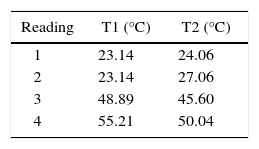
Sophisticated measuring equipment has been used to measure air temperature and pressure within the turbulent region. The propagation path length is represented by L and is equal to 2.52 m; the wavenumber k is the wavelength of a helium-neon laser at 532 nm; r describes the region between two reference points within the propagation path length, and T₁ and T₂ represent the temperatures at the two reference points. Measuring these observations in the laboratory allows one to determine, after Andrews and Phillips, 1998),

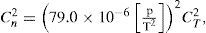
with

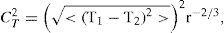
where Cn2 represents the temperature structure function.

As the laser beam propagates through the inhomogeneous medium, the turbulence created within the wind tunnel presents itself as small packets of air, also known as turbulent eddies. Each turbulent eddy has a unique refractive index which affects the laser beam differently. Holistically we can obtain the general strength of the turbulent region using Eq. (1). Typical values of C² range from 10⁻¹⁷ m^−2/3 or less for weak turbulences to 10⁻¹³ m^−2/3 or more for strong turbulence (Andrews et al., 2005; Weichel, 1990). Other characterizing features of the atmosphere can also be classified by the Reynolds number and seeing conditions (Fried's parameter). The Reynolds number is given by

where u is the mean velocity, v is the kinematic viscosity of the fluid and l, the path length. We can relate the index function to Fried's parameter through Magee (1993),

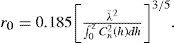
Determining the seeing conditions at low altitude may result in very low values (less than 5 cm) as the quantity alone describes the quality of the optical signal through the atmosphere. At high altitudes, such as an observatory which is clear from high levels of atmospheric contrasts, values of r₀ between 5 and 20 cm should be obtained.

3

Experimental setup

A diagrammatic description of the components is presented in Figure 1.

Fig. 1.

2D view of the experimental setup. A more detailed design of the wind tunnel is presented in Figure 2.

The experimental setup used in this work was adapted from a previous work by Ndlovu and Chetty (2015). We have chosen to use a laboratory setup as it removes inconsistencies of the atmosphere, such as varying wind velocities, temperatures and flow directions. Once the setup is able to detect and quantify the effects of simulated atmospheric turbulence, it can be moved to the outside. A turbulence generator and a chamber have been designed for the laboratory setup but the characteristics of the turbulence generator are designed to mimic real world atmospheric turbulence. By introducing a wind element into the setup, a new technique for characterizing the laser beam will be explored. As with previous works by Ndlovu and Chetty (2015) and Augustine and Chetty (2014), we set out to minimize the cost and time devoted to our testing procedures.

To recreate atmospheric wind, a fan connected to a high powered motor was used. The fan blades spin at high velocity producing a consistent stream of air which propagates perpendicularly to the motion of the laser beam. The air was immediately heated by a coil which can be operated at two power settings, 1000 and 2000 W. The characteristics of air speed, air temperature and pressure were measured at the exit of the tunnel at a distance of 36 mm along the length of the testing region (refer to Fig. 2). The resultant perturbed beam was then photographed and the statistical properties of the perturbation measured.

Fig. 2.

Depiction of the wind tunnel.

4

Experimental procedure

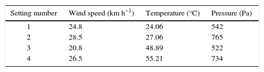
The optical components were first checked to ensure that they are free of any dust particles. The laser is thereafter given sufficient time to warm up and stabilize. The laser alignment is also checked so that it propagates directly through the optical components. The wind turbine was given sufficient time to run before measurements began. The heating element had four possible settings. Table I describes each setting and provides the temperature and corresponding characteristics of the wind tunnel.

Table I.

Wind speed vs. temperature.

Setting number	Wind speed (km h^−1)	Temperature (°C)	Pressure (Pa)
1	24.8	24.06	542
2	28.5	27.06	765
3	20.8	48.89	522
4	26.5	55.21	734

Settings 1 and 2 represent two variations in wind speed with no additive heat, i.e., high velocity room temperature wind. It was necessary to determine if there was any influence on the laser beam with the heat element removed. The results are presented in the next section.

5

Results, analysis and discussion

5.1

Reading 1

For comparison, the unperturbed interferogram is presented in Figure 3. Figures 3 to 6 present the results for the unperturbed interferogram.

Fig. 3.

Unperturbed interferogram.

Fig. 4.

Unperturbed intensity distribution.

Fig. 5.

Magnitude of the fast Fourier transform (FFT).

Fig. 6.

Point spread function.

Reading 1 will be the basis of comparison against the other readings, as it represents a laser beam propagating through a homogeneous medium with no applied turbulence (thermally or directionally). Determining the differences in the interferograms, intensity profiles, fast Fourier transforms (FFT) and image subtractions will provide us with insight into how the laser beam reacts under low and high turbulent strain. The turbulence generated in the laboratory could typically represent aerodynamical configurations experienced in the atmosphere by airborne platforms (Magee, 1993). Figure 3 presents a clearly defined interferogram which exhibits a uniform distribution of energy over the area of the laser beam. Figure 4 expresses the intensity profile which resembles a Gaussian profile, which is expected since the beam is unperturbed. The dip in the center can be attributed to stray artifacts arising from either the neutral density or spatial filter. Figure 5 is the FFT, which was used as it resolves the image into its magnitude and phase domains. The magnitude is useful for image processing since all the frequencies that compose the image are specified.

We will restrict ourselves to the magnitude domain, as the frequency domain does not provide us with sufficient information. Making reference to Figure 5, the image is formed on a 2D plane in polar representation and shows that there is a high concentration of frequencies at the center of the image. The image contains various frequency components which decrease slowly for larger frequencies. The central bright spot is known as the zero frequency zone or direct current zone and represents the average color value of the entire image (Banish, 1990). Additionally, the image does not contain imaginary components and, thus the magnitude at the center has a zero phase resulting in a gray spot. The large concentration around the center point indicates a lower spatial frequency (Banish, 1990).

Numerous adjustments can be made to the transformed image to either improve the focus or decrease blurriness, which can be achieved by applying a low pass filter to preserve the low frequency regions, or a high pass filter to preserve the sharpness and defined edges. Intermittent filters, known as band pass filters, can be applied. For comparisons in subsequent readings we will compare their FFTs to Figure 5 by image subtraction. If the subtraction yields a completely black image, it is implied that the two images coincide completely, hence there is no change in beam position, distortion, blurriness or phase.

5.2

Reading 2

Setting 1 describes the scenario of a moderately windy day at 20.5 °C. Figures 7 to 10 present the results for the perturbation at turbulence setting 1.

Fig. 7.

Setting1, perturbed interferogram.

Fig. 8.

Setting 1, intensity distribution.

Fig. 9.

Setting 1, magnitude of the FFT.

Fig. 10.

Setting 1, image subtraction.

The results displayed are those of the perturbed laser beam being exposed to a 24.8 km h⁻¹ wind velocity at a room temperature of 24.06 °C. In Figure 7 we can see that dark fringes are less defined and that interferogram is blurred when compared to Figure 3. Figure 8 shows energy redistribution over the area of the interferogram and also a maximum peak intensity of 220 units over the initial unperturbed value of 255 units. Although the intensity is only 35 units lower, there is a total redistribution of energy over the peaks. The FFT magnitude in Figure 9 shows a small collection of the lower spatial range in the center, which suggests a somewhat similar spatial distribution as the unperturbed beam. This means that despite the distortion and blurriness of the interferogram, the spatial domain has been altered (Banish, 1990). Compared to Figure 5, the collection of lower frequencies is significantly less but not entirely substantial. The image subtraction data in Figure 10 shows us the lower spatial region, which has been either shifted to higher frequencies or lost during propagation. Overall, the beams characteristics are still strong and possess qualities of their initial forms.

5.3

Reading 3

Figures 11 to 14 present the results for the perturbation at turbulence setting 2.

Fig. 11.

Setting 2, perturbed interferogram.

Fig. 12.

Setting 2, intensity distribution.

Fig. 13.

Setting 2, magnitude of the FFT.

Fig. 14.

Setting 2, image subtraction.

Reading 3 was conducted at the highest speed setting achievable by the wind turbine at 28.50 km h⁻¹ and at a room temperature of 27.06 °C. The higher room temperature is due to the much higher ambient temperature within the laboratory. Despite the increase in turbine speed, visual changes are the most significant. Propagation path length and altitude remain the same as in other testings. The fringes are slightly lighter signifying that the beam is experiencing directional fluctuations and is shifting over the PDI membrane. The intensity profile in Figure 12 shows approximately the same drop in peak power as in Figure 8. Additionally, the FFT magnitude (Fig. 13) and image subtraction (Fig. 14) present similar data to reading 1. This implies that the beam suffered minor changes with an increase in wind speed of 3.7 km h⁻¹. The high localization of the lower spatial region implies minimal directional deviation from the initial unperturbed interferogram. The image subtraction data shows that energy as well as directional fluctuations are evident, as seen by the gray pixels existing from the middle to the center of the image. Future work will entail building a larger wind tunnel which can simulate wind speeds of up to 100 km h⁻¹. Small scale tests are necessary to determine if the PDI can measure small scale simulations.

5.4

Reading 4

Figures 15 to 18 present the results for the perturbation at turbulence setting 3.

Fig. 15.

Setting 3, perturbed interferogram.

Fig. 16.

Setting 3, intensity distribution.

Fig. 17.

Setting 3, magnitude of the FFT.

Fig. 18.

Setting 3, image subtraction.

In reading 4 a single 1000 W coil was used, which heated the air significantly to 48.89 °C and at a wind velocity of 20.8 km h⁻¹. Readings were taken and averaged after approximately 10 min. The interferogram in Figure 15 describes a severely distorted, blurred image. The fringes are completely deformed, faint and out of focus when compared to the unperturbed interferogram. The directional shift of the laser beam has caused the laser to propagate through more than one PDI pinhole, causing the constructive and destructive fringes. The intensity profile in Figure 16 shows that peak intensity reaches 145 pixel units from a maximum value of 254 pixel units, a drop of 43% in intensity. Despite the somewhat Gaussian distribution, it is interesting to note that the intensity is redistributed over the beam. The image subtraction (Fig. 17) shows an almost absent lower spatial region. The frequencies are random and encompass the entire area of the beam. This signifies a complete redistribution directionally and spatially. Banish, 1990 described this behavior to result in image blur and deformation, which is evident from the interferogram. Figure 18 presents the difference in the lower spatial localization from the initial unperturbed data. This simulation has caused the beam to lose many of the basic characteristics of a He-Ne laser, such as having a high coherence and directional forte. However, the energy distribution still describes a Gaussian profile but with significantly less energy.

5.5

Reading 5

Figures 19 to 22 present the results for the perturbation at turbulence setting 4.

Fig. 19.

Setting 4, perturbed interferogram.

Fig. 20.

Setting 4, intensity distribution.

Fig. 21.

Setting 4, magnitude of the FFT.

Fig. 22.

Setting 4, image subtraction.

Reading 5 utilizes the highest speed and temperature capabilities of the wind turbine. Within the turbulent region, the air is heated to 55.21 °C and it moves at a velocity of 26.5 km h⁻¹. Even though the wind speed has increased only slightly, the 6.3 °C heat increase has rendered the laser beam to be almost completely unidentifiable. Figure 19 describes a highly affected beam which has no focus, shape or form. This is due to its loss of coherence, direction and intensity. It is interesting to note how quickly the laser beam completely loses its basic characteristics with an increase in temperature variation. The intensity profile (Fig. 20) resembles an erratic trend, which suggests that the beam has experienced various energy redistributions over the entire profile. The peak intensity has dropped to 76 pixel units from the original value of 254 pixel units. This defines an extreme loss in energy of approximately 70%. Figure 21 presents the FFT and shows a complete loss of the beams lower spatial frequency just as in reading 4. The phases of the laser beam are inconsistent and do not follow a consistent distribution as would be expected. Figure 5 reinforces the expectations of the He-Ne Gaussian profile to have a defined lower spatial domain (Banish, 1990; Fried, 1965). The image subtraction data in Figure 22 reveals a grey central region which shows the difference in the lower spatial frequency redistribution when compared to Figure 5. The exposure of the beam to such heat with wind velocity has caused the loss of all its basic characteristics. In this case, the intensity has dropped so low that only 30% of its initial energy has reached the detector. Any further simulations above this temperature may lead to more severe implications and possibly an eventual loss of all energy.

6

Determination of Cn2

To measure the refractive index of the atmosphere within the turbulent region, a few parameters are required, namely temperature (T₁ and T₂), pressure (p) and separation distance (r = 72 mm). In this work, four averaged readings were taken, the first two being variations of high wind velocity without additive heat, and the second being two variations of wind velocity and heat. Tables I and II present the parameters.

Table II.

Atmospheric parameters.

Reading	T1 (°C)	T2 (°C)
1	23.14	24.06
2	23.14	27.06
3	48.89	45.60
4	55.21	50.04

Data in Tables I and II are used to determine the refractive index structure function, temperature structure function and seeing parameter with the use of Eqs. (1), (2) and (3), respectively.

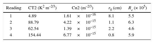
The results in Table III compare well with numerous published data for similar atmospheric scenarios (Weichel, 1990; Kemp et al., 2001; Ndlovu, 2013; Tunick et al., 2005). Our results for Cn2 can be classified under the moderate to strong turbulence regime (Andrews et al., 2005). Our measuring apparatus have allowed us to precisely determine these structure functions accurately. Values for Cn2 vary from one source to the other and depend largely on the logistics of the atmosphere, the position above ground, the separation distance between measuring points and the consistency of the temperature over the path length. For short path lengths such as the one used in this experiment, the turbulence can be accurately determined due to the stability of the atmosphere within the laboratory. The seeing parameter ranges between 8.1 and 0.8 cm (Kemp et al., 2001). Decreasing values of r₀ result in increasing phase distortions of the laser beam as well as an increasing degradation of the atmosphere. This claim has been extensively reviewed in the analysis of readings 2 to 5. Another parameter which is often used to classify the flow of the atmosphere is the Reynolds number. From data in Table III, the Reynolds number describes a highly turbulent flow and implies that for a consistent medium, an increase in measured air speed over a measured distance will result in a proportional increase in the Reynolds number.

Table III.

Temperature and refractive index structure function data.

Reading	CT2 (K^2 m^–2/3)	Cn2 (m^–2/3)	r0 (cm)	Re (× 10^5)
1	4.89	1.61 × 10^−16	8.1	5.5
2	88.79	4.22 × 10^−15	1.1	6.3
3	62.54	1.39 × 10^−15	2.2	4.6
4	154.44	6.77 × 10^−15	0.8	5.9

6.1

Error analysis

The experimental error arises from both systematic and random contributions. Systematic errors occur from the miscalibration of measuring apparatus. The PDI controller has been quoted at 95% accuracy; hence, a maximum error of 5% can be expected. The pressure sensor quotes a maximum possible error of 0.1 Pa or a 1% error. The thermocouple states a precision of 0.1 °C which is approximately a 1% error. The anemometer quotes a 1% total error. Although these errors are expected from the measuring instruments we have averaged our data over thousands of simulations, therefore the mean would be an estimate of the true result. Random errors occur through dust particulate in the air, vibrations in the floor or any random air currents exiting during simulations. Our laboratory environment has been sealed off to allow minimal dust, vibration or air currents into the testing region. We can therefore assume a precision accuracy of 95% in our results. The error bar chart of the new C² range is provided in Figure 23.

Fig. 23.

Refractive index variations for readings 2-5.

7

Conclusions

Our results prove that the PDI was able to detect and produce quantifiable interferograms. Thousands of readings were taken and averaged into four separate settings, two being variations of wind speed at room temperature and the remaining two being heat settings at two possible wind speeds. All perturbed readings were compared against the unperturbed results to measure the differences and effects. In summary, readings 2 and 3 showed signs of image blur, minor beam wander, and minor beam spreadings, however both held a strong intensity profile. This implies that wind velocity alone does not destroy all the beams characteristics. Readings 4 and 5 were nevertheless severely affected by the accompanying heat included in the wind stream. Both showed an extreme loss of coherence, direction and intensity. Reading 5 exhibited no basic elements of the initial unperturbed analysis and was almost uncharacterizable. Smaller values relate to an increasingly degraded atmosphere. With this in mind, we can conclude that heat perturbations were significantly more severe than perturbations with wind velocity alone. The additive effect showed the beam to be severely degraded in terms of power loss as well as directional fluctuations. In previous works by Augustine and Chetty (2014), data was provided for a heated panel as a turbulent source. The results vary with respect to this work, since the contributions from directional fluctuations were minimal. As such, we can conclude that heat contributions alone do not affect the laser beam as significantly as directional perturbations. To further classify the atmosphere within the turbulent region we determined the refractive index structure function, which ranged from 1.61 × 10⁻¹⁶ to 6.77 × 10⁻¹⁵. This falls under the moderate to strong turbulence regime. The seeing parameter was also calculated and found to be 8.1 to 0.8 cm. Future work entails developing a liquid bath through which the laser beam will propagate. We wish to determine how the laser beam reacts through different liquids as well as through varying liquid temperatures. Other detection and analysis methods will also be explored to best suit the experimental design and expectations.