Regional frequency analysis of daily rainfall extremes using L-moments approach

Resumen

Los valores extremos de precipitación diaria se encuentran entre los sucesos ambientales con consecuencias más desastrosas para la sociedad. La información sobre las magnitudes y frecuencias de las precipitaciones extremas es vital para el manejo sostenible de los recursos hídricos, la planeación de emergencias vinculadas con el clima y el diseño de estructuras hidráulicas. En este trabajo se analiza la frecuencia de precipitaciones diarias máximas en la provincia de Golestán, localizada en el noreste de Irán. Se trataron de encontrar distribuciones de frecuencias regionales adecuadas para precipitaciones máximas diarias y de predecir los valores de retorno de episodios extremos de precipitación (diseño de la profundidad de la precipitación). Se aplicó la regionalización de procedimientos de momentos-L, en conjunto con un método de indización de las precipitaciones, a los registros máximos de precipitación de 47 estaciones en el área de estudio. Debido a las complejas características geográficas e hidroclimatológicas de la región, un aspecto importante de la investigación fue la desagregación del área en subregiones coherentes y homogéneas. Así, se dividió el área de estudio en cinco regiones homogéneas con base en análisis de conglomerados de las características locales y en pruebas de homogeneidad regional. Los resultados de la precisión del ajuste indicaron que la mejor distribución es diferente para cada región homogénea. La diferencia puede deberse a las condiciones climáticas y geográficas distintivas de cada región. Los cuantiles regionales estimados y sus medidas de precisión, obtenidas mediante simulaciones de Monte Carlo, demuestran que la estimación de incertidumbre mediante valores de la raíz cuadrada del error cuadrático medio (RMSE, por sus siglas en inglés) y límites del error estadístico de 90%, es relativamente baja cuando los periodos de retorno son menores de 100 años. Sin embargo, para periodos más largos, las estimaciones de precipitación deben tomarse con cautela. Más años por estación, ya sea por registros más largos o por más estaciones en las regiones, se requerirían para estimaciones de precipitación mayores a T = 100 años. El análisis encontró que el índice de precipitación (promedio in situ de la máxima precipitación) puede estimarse razonablemente bien como una función de la precipitación media anual en la provincia de Golestán. Pueden utilizarse índices de precipitación combinados con curvas de crecimiento regional para calcular precipitaciones de diseños en sitios carentes de sistemas de medición. En general se encontró que el análisis de conglomerados, en conjunto con la técnica de análisis regional de frecuencias basada en momentos-L, puede aplicarse de manera exitosa para obtener estimados de precipitaciones de diseño en el noreste de Irán. El enfoque de este trabajo y sus resultados tienen gran importancia científica y mérito práctico, en particular para la planeación de emergencias relacionadas con el clima y el diseño de estructuras hidráulicas.

Abstract

Daily extreme precipitation values are among environmental events with the most disastrous consequences for human society. Information on the magnitudes and frequencies of extreme precipitations is essential for sustainable water resources management, planning for weather-related emergencies, and design of hydraulic structures. In the present study, regional frequency analysis of maximum daily rainfalls was investigated for Golestan province located in the northeastern Iran. This study aimed to find appropriate regional frequency distributions for maximum daily rainfalls and predict the return values of extreme rainfall events (design rainfall depths) for the future. L-moment regionalization procedures coupled with an index rainfall method were applied to maximum rainfall records of 47 stations across the study area. Due to complex geographic and hydro-climatological characteristics of the region, an important research issue focused on breaking down the large area into homogeneous and coherent sub-regions. The study area was divided into five homogeneous regions, based on the cluster analysis of site characteristics and tests for the regional homogeneity. The goodness-of-fit results indicated that the best fitting distribution is different for individual homogeneous regions. The difference may be a result of the distinctive climatic and geographic conditions. The estimated regional quantiles and their accuracy measures produced by Monte Carlo simulations demonstrate that the estimation uncertainty as measured by the RMSE values and 90% error bounds is relatively low when return periods are less than 100 years. But, for higher return periods, rainfall estimates should be treated with caution. More station years, either from longer records or more stations in the regions, would be required for rainfall estimates above T=100 years. It was found from the analyses that, the index rainfall (at-site average maximum rainfall) can be estimated reasonably well as a function of mean annual precipitation in Golestan province. Index rainfalls combined with the regional growth curves, can be used to estimate design rainfalls at ungauged sites. Overall, it was found that cluster analysis together with the L-moments based regional frequency analysis technique could be applied successfully in deriving design rainfall estimates for northeastern Iran. The approach utilized in this study and the findings are of great scientific and practical merit, particularly for the purpose of planning for weather-related emergencies and design of hydraulic engineering structures.

1

Introduction

Extreme environmental events can have substantial impacts on society and the economy (Shabri et al., 2011). Extreme high precipitation amounts are among environmental events with the most disastrous consequences for human society (Kysely et al., 2006). Information on the magnitudes and frequencies of extreme precipitations is essential for sustainable water resources management, planning for weather-related emergencies, design of hydraulic structures (e.g., flood protection structures, urban drainage systems, and irrigation ditches), agricultural management, and for studies related to weather modification and climatic change (Durrans and Kirby, 2004).

In order to minimize the risk and maximize efficiency in design, statistical and probabilistic methods are applied to past events for predicting the exceedance probability of future events (Smithers and Schulze, 2001). However, reliable estimations require very long station records if single station data are to be used. Regional frequency analysis (RFA) is therefore used to provide a framework for hazard characterization of the extreme events (Norbiato et al., 2007). The regionalization concept "trades space for time" by using data from nearby or similar sites, in order to estimate quantiles of the underlying variable at each site in the homogeneous region of consideration (Dalrymple, 1960; Norbiato et al., 2007).

The earliest effort in regional frequency analysis is the work of Dalrymple (1960), who introduced the concept of regionalization. The concept was continuously developed and new approaches were further introduced and investigated by other researchers (e.g. Vicens et al., 1975; Greiss and Wood, 1981; Rossi et al., 1984; Lettenmaier et al., 1987; Burn, 1990; Stedinger and Lu, 1995; Hosking and Wallis, 1997; Sveinsson et al., 2001; Norbiato et al., 2007; González and Valdés, 2008; Meshgi and Khalili, 2009a, b). Techniques which have been widely applied in rainfall regionalization (cit. by Ngongondo et al., 2011) include: linkage analysis (e.g. Jackson, 1972); spatial correlation analysis (Gadgil et al., 1993); common factor analysis (e.g. Barring, 1988); empirical orthogonal function analysis (e.g. Kulkarni et al., 1992); principal component analysis (PCA) (e.g. Baeriswyl and Rebetez, 1996; Singh and Singh, 1996); cluster analysis (e.g. Easterling, 1989; Venkatesh and Jose, 2007); combination of PCA and cluster analysis (e.g. Dinpashoh et al., 2004); L-moments associated with cluster analysis (e.g. Schaefer, 1990; Guttman, 1993; Wallis et al., 2007; Satyanarayana and Srinivas, 2008); a combination of L-moments and generalized least squares regression (Haddad et al., 2010); Bayesian generalized least squares (Johnson et al., 2012) and regional flood frequency analysis using L-moments in Iran (e.g. Malekinezhad et al., 2010, 2011).

Among different methods of regional frequency analysis, the regional index-flood type approach based on L-moments (Hosking and Wallis, 1993,1997) has many reported benefits and has the potential of unifying current practices of regional design rainfall analysis (Smithers and Schulze, 2001). This technique is used at all stages of regional analysis including: identification of homogeneous regions, identification and testing of regional frequency distributions, and estimations of parameters and quantiles at stations of interest.

The Golestan province is one of the 31 provinces of Iran, located in the northeast of the country, to the southwest of the Caspian Sea. It is an important region for agricultural production, especially cotton, and plays an important role in the sustainable development of the economy and ecology of northern Iran. However, this area has many flood-related problems and has become the most affected province of Iran. Over the past 10 years, extreme precipitation events have contributed to an increase in the frequency of flash floods in this area. During the first half of the 2000-2010 decade, Golestan experienced the most deadly flash floods in its recorded history (Sharifi et al., 2011). On August 10, 2001 an extreme storm and flood occurred in the eastern part of the province, as a result of a nearly 10-hour rainfall with 170 mm depth. Based on the information reported by the Dartmouth Observatory Global Flood Archive up to August 2001, more than 243 people died, more than 190 people were lost, and the property losses were estimated over USD 77.25 millions (MAB, 2001). Another catastrophic storm and flood occurred on August 13, 2002, which led to 42 deaths and 30 missing persons. The floods of 2005, which occurred on July 30 and August 9, destroyed many structures that were rehabilitated after the 2001 and 2002 floods.

Considering the storm/flood related problems of the Golestan province, the analysis of extreme rainfall data can be utilized by decision makers to setup measures for reducing the impact of the disaster. Therefore, in the present study, an attempt has been made to analyze the regional frequency of extreme rainfall events for the Golestan province, using the annual series of maximum daily rainfall data and the well-known L-moments approach.

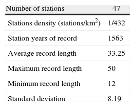
2

Materials and methods

2.1

Study area and data

With an area of 20 311.6 km², the Golestan province is situated in the southeast of the Caspian Sea, covering about 1.3% of the total area of Iran. The province is located between 36° 44’-38° 05’ north latitude and 53° 51’-56° 14’ east longitude. It has an altitude range from -28 to 3945 masl and a mean slope of 35.82%. The main perennial rivers are Gorganrood, Atrak and Ghare-sou, which are among the most important rivers of the Caspian Sea river basin. The rivers originate in the Alborz Mountains, flow from east to west and finally enter the Caspian Sea from the eastern coast.

Since the area of consideration is located between the Caspian Sea and the Alborz Mountains, the climate of this area is generally moderate. The average annual temperature is 18.2 °C and the annual rainfall is about 550 mm. Precipitation displays a considerable temporal and spatial variability in the province. Annual rainfall totals, in general, a decrease from south to north and precipitation mostly occurs during winter and spring. The sub-climatic classification of the region is as follows: the northern part, moderate to dry; the central flat and mountainous areas, moderate semi-dry to semi-wet; and the southern mountainous areas, cold semi-wet to cold semi-dry. In recent years, flooding triggered by heavy rainfall produced lots of human deaths and financial losses to residents of the province. Recent flooding events resulting from heavy rainfalls occurred in 2001, 2002, 2005, and 2008.

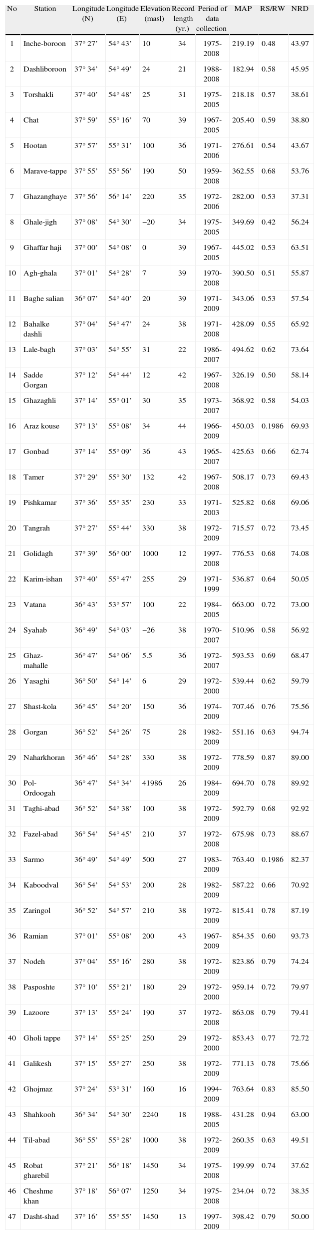
In the present study, daily rainfall data of 47 gauge stations, compiled by the Iranian Meteorological Organization and also by regional water resources departments, have been analyzed. The study was limited, by necessity, to daily data, as sub-daily data are not generally available with sufficient coverage and length of record. New time series of annual maximum daily data are then abstracted from these daily data. In addition, information on longitude, latitude, and mean elevation above sea level was also obtained for each site. Figure 1 shows the location of the Golestan province and the 47 rainfall gauge stations, with basic information presented in Tables I and II.

Fig. 1.

Location of the Golestan province and rainfall stations used in the regional frequency analysis.

Table I.

List of the 47 rain gauge stations and associated characteristics in the Golestan province.

No	Station	Longitude (N)	Longitude (E)	Elevation (masl)	Record length (yr.)	Period of data collection	MAP	RS/RW	NRD
1	Inche-boroon	37° 27’	54° 43’	10	34	1975-2008	219.19	0.48	43.97
2	Dashliboroon	37° 34’	54° 49’	24	21	1988-2008	182.94	0.58	45.95
3	Torshakli	37° 40’	54° 48’	25	31	1975-2005	218.18	0.57	38.61
4	Chat	37° 59’	55° 16’	70	39	1967-2005	205.40	0.59	38.80
5	Hootan	37° 57’	55° 31’	100	36	1971-2006	276.61	0.54	43.67
6	Marave-tappe	37° 55’	55° 56’	190	50	1959-2008	362.55	0.68	53.76
7	Ghazanghaye	37° 56’	56° 14’	220	35	1972-2006	282.00	0.53	37.31
8	Ghale-jigh	37° 08’	54° 30’	−20	34	1975-2005	349.69	0.42	56.24
9	Ghaffar haji	37° 00’	54° 08’	0	39	1967-2005	445.02	0.53	63.51
10	Agh-ghala	37° 01’	54° 28’	7	39	1970-2008	390.50	0.51	55.87
11	Baghe salian	36° 07’	54° 40’	20	39	1971-2009	343.06	0.53	57.54
12	Bahalke dashli	37° 04’	54° 47’	24	38	1971-2008	428.09	0.55	65.92
13	Lale-bagh	37° 03’	54° 55’	31	22	1986-2007	494.62	0.62	73.64
14	Sadde Gorgan	37° 12’	54° 44’	12	42	1967-2008	326.19	0.50	58.14
15	Ghazaghli	37° 14’	55° 01’	30	35	1973-2007	368.92	0.58	54.03
16	Araz kouse	37° 13’	55° 08’	34	44	1966-2009	450.03	0.1986	69.93
17	Gonbad	37° 14’	55° 09’	36	43	1965-2007	425.63	0.66	62.74
18	Tamer	37° 29’	55° 30’	132	42	1967-2008	508.17	0.73	69.43
19	Pishkamar	37° 36’	55° 35’	230	33	1971-2003	525.82	0.68	69.06
20	Tangrah	37° 27’	55° 44’	330	38	1972-2009	715.57	0.72	73.45
21	Golidagh	37° 39’	56° 00’	1000	12	1997-2008	776.53	0.68	74.08
22	Karim-ishan	37° 40’	55° 47’	255	29	1971-1999	536.87	0.64	50.05
23	Vatana	36° 43’	53° 57’	100	22	1984-2005	663.00	0.72	73.00
24	Syahab	36° 49’	54° 03’	−26	38	1970-2007	510.96	0.58	56.92
25	Ghaz-mahalle	36° 47’	54° 06’	5.5	36	1972-2007	593.53	0.69	68.47
26	Yasaghi	36° 50’	54° 14’	6	29	1972-2000	539.44	0.62	59.79
27	Shast-kola	36° 45’	54° 20’	150	36	1974-2009	707.46	0.76	75.56
28	Gorgan	36° 52’	54° 26’	75	28	1982-2009	551.16	0.63	94.74
29	Naharkhoran	36° 46’	54° 28’	330	38	1972-2009	778.59	0.87	89.00
30	Pol-Ordoogah	36° 47’	54° 34’	41986	26	1984-2009	694.70	0.78	89.92
31	Taghi-abad	36° 52’	54° 38’	100	38	1972-2009	592.79	0.68	92.92
32	Fazel-abad	36° 54’	54° 45’	210	37	1972-2008	675.98	0.73	88.67
33	Sarmo	36° 49’	54° 49’	500	27	1983-2009	763.40	0.1986	82.37
34	Kaboodval	36° 54’	54° 53’	200	28	1982-2009	587.22	0.66	70.92
35	Zaringol	36° 52’	54° 57’	210	38	1972-2009	815.41	0.78	87.19
36	Ramian	37° 01’	55° 08’	200	43	1967-2009	854.35	0.60	93.73
37	Nodeh	37° 04’	55° 16’	280	38	1972-2009	823.86	0.79	74.24
38	Pasposhte	37° 10’	55° 21’	180	29	1972-2000	959.14	0.72	79.97
39	Lazoore	37° 13’	55° 24’	190	37	1972-2008	863.08	0.79	79.41
40	Gholi tappe	37° 14’	55° 25’	250	29	1972-2000	853.43	0.77	72.72
41	Galikesh	37° 15’	55° 27’	250	38	1972-2009	771.13	0.78	75.66
42	Ghojmaz	37° 24’	53° 31’	160	16	1994-2009	763.64	0.83	85.50
43	Shahkooh	36° 34’	54° 30’	2240	18	1988-2005	431.28	0.94	63.00
44	Til-abad	36° 55’	55° 28’	1000	38	1972-2009	260.35	0.63	49.51
45	Robat gharebil	37° 21’	56° 18’	1450	34	1975-2008	199.99	0.74	37.62
46	Cheshme khan	37° 18’	56° 07’	1250	34	1975-2008	234.04	0.72	38.35
47	Dasht-shad	37° 16’	55° 55’	1450	13	1997-2009	398.42	0.79	50.00

MAP: mean annual precipitation; RS/RW: mean ratio of summer half-year precipitation to winter half-year precipitation; NRD: mean annual number of rainy days

Table II.

Rain-gauge network information for the study area

Number of stations	47
Stations density (stations/km^2)	1/432
Station years of record	1563
Average record length	33.25
Maximum record length	50
Minimum record length	12
Standard deviation	8.19

2.2

Preliminary data analysis

Stationarity and independence are important underlying assumptions inherent to frequency analysis. Without stationary and serial correlation tests, the analysis may lead to incorrect results and conclusions. Another requirement is that data at different stations in a homogeneous region should be spatially independent. High spatial cross-correlation between stations gives a lower degree of additional regional information to the site being studied than uncorrelated sites (Ngongondo et al., 2011). Stationarity was examined using the nonparametric Mann-Kendall (MK) trend test (Mann, 1945; Kendall, 1975); independence was tested using lag-1 to lag-5 autocorrelation coefficients, and Moran’s I (Moran, 1950) was used to test for spatial independence.

2.3

Regional frequency analysis methodology

The methodology used here for regional frequency analysis of maximum daily rainfalls in the Golestan province is an index variable approach based on L-moments as outlined by Hosking and Wallis (1997). This approach involves five main steps: (1) identification of candidate homogenous regions by cluster analysis; (2) screening of the data using the discordancy measure Di; (3) homogeneity testing using the heterogeneity measure H; (4) distribution selection using the L-moments ratio diagram and the goodness-of-fit measure Z; and (5) regional estimation of rainfall quantiles using the L-moment approach.

2.4

Identification of candidate homogenous regions

The configuration of candidate homogenous regions was based on cluster analysis, in which a vector of site characteristics is associated with each site and standard multivariate statistical analysis is performed on group sites according to the similarity of the vectors (Hosking and Wallis, 1997). The following site characteristics were used in the cluster analysis: longitude, latitude, elevation, mean annual precipitation, mean ratio of summer half-year precipitation to winter half-year precipitation, and mean annual number of rainy days. These site characteristics are considered to be important in defining a site’s precipitation climate; they include indicators of precipitation amounts, distributions of the amounts through the year, and geographic location.

Most clustering algorithms are very sensitive to the Euclidean distance or scale of the variables used in the analysis (Hosking and Wallis, 1997;Smithers and Schulze, 2001). To avoid dominance of site characteristics with large absolute values (e.g., altitude), the variables were rescaled so that their values would lie between 0 and 1.

Ward’s minimum variance hierarchical clustering algorithm (Ward, 1963), which is reported to be useful for the identification of homogeneous regions in a regionalization process (Hosking and Wallis, 1997; Rao and Srinivas, 2008), was applied to cluster analysis. The appropriate number of groups (clusters) was determined using the silhouette widths and Mantel comparison methods (Borcard et al., 2011).

2.5

Testing for homogeneity of the regions

Hosking and Wallis (1993) derived two statistics to test the homogeneity of a region. The first statistic, discordancy measure (D_i), is a measure of dissimilarity. D_i is a statistic based on the difference between L-moment ratios of a site and the average L-moment ratios of a group of similar sites. This statistic can also be used to identify erroneous data. The discordancy measure for site i is defined as follows:

where u_i is a vector containing three L-moment ratios (i.e., L-Cv, L-skewness and L-kurtosis) for site i, u is the vector containing the simple average L-moment ratios, and S is the sample covariance matrix of L-moments of all sites. Generally, any site with D_i > 3 is considered discordant (Hosking and Wallis, 1993; Adamowski, 2000).

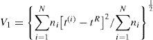
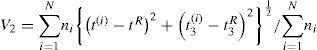
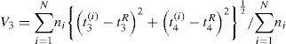
The second criterion, called H-statistic, is a measure of heterogeneity. This statistic compares the between-site variability (dispersion) of L-moments with what would be expected for a homogeneous region. To determine what would be expected, repeated Monte Carlo simulations of a homogeneous region with sites having record lengths equal to those of the observed data are performed. The test compares the variability of L-statistics of the actual region to those of the simulated series. There are three heterogeneity measurers, namely H₁, H₂ and H₃, which are calculated using the following equation:

where µ_V and σ_V are the mean and standard deviation of Nsim values of V (Nsim is the number of simulation data). V_i is calculated from the regional data, based on the corresponding V-statistic defined as follows: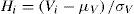

A region is declared "acceptably homogeneous" if H < 1, “possibly heterogeneous" if 1 ≤ H < 2, and “definitely heterogeneous” if H ≥ 2 (Hosking and Wallis, 1997).

2.6

Identifying the regional frequency distribution

The regional frequency distribution is chosen based on the L-moment ratio diagram and the goodness-of-fit measure Z^Dist. The goodness-of fit measure judges how well the theoretical L-kurtosis of a fitted distribution matches the regional average L-kurtosis of the observed data. For each candidate distribution, Z^Dist is calculated as follows:

where t4R is an average L-kurtosis value computed from the data of the region, τ4Dist is a theoretical L-kurtosis value computed from the simulation for a fitted distribution, and σ₄ is the standard deviation of L-kurtosis values obtained from simulated data. The fit of a distribution is considered satisfactory if |Z^Dist| ≤ 1.64. When more than one distribution qualifies for the goodness-of-fit measure, the preferred distribution will be the one that has the minimum |Z^Dist|value.

2.7

Estimation of regional rainfall quantiles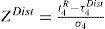

Once the appropriate frequency distribution for each homogeneous region is identified, quantiles are estimated for several probability levels or return periods using the index rainfall method. The procedure assumes maximum daily rainfall data at different sites in a homogeneous region have the same distribution, except for a site-specific scale parameter or an index factor (Dalrymple, 1960). The scale factor is appointed as an index-rainfall and is generally taken to be the mean of annual maximum daily rainfall. The quantile estimates QˆF with non-exceedance probability F at a site in a region with N sites are computed by: QiF=liqF, where q is a common dimensionless quantile function (regional growth curve) and l₁ is the index rainfall value, representing the T-year quantile of the normalized regional distribution (Ngongondo et al., 2011). Using the regional parameters for the identified distribution, the regional growth curve is computed and multiplied by the station specific average annual maximum rainfall to obtain the desired rainfall quantiles for the relevant station.

The accuracy of estimated rainfall quantiles is assessed using Monte Carlo simulations (Hosking and Wallis, 1997). For each homogeneous region, a region is simulated having the same number of stations, record length at each station, heterogeneity, and regional average L-moment ratios as the observed data. This procedure was repeated 1000 times, to obtain 1000 simulated regions. For each simulation, errors in the simulated growth curve and quantiles were calculated and then the bias, root mean square error (RMSE), and 90% error bounds estimated. Computation details for the accuracy assessment can be found in Hosking and Wallis (1997).

All statistical computations and graphical displays were made using R statistical software version 2.15.0. The R package lmomRFA developed by Hosking (2009) was used for L-moment analysis.

3

Results and discussion

3.1

Test for stationarity and independence

The preliminary process of data (i.e., examining the stationarity, serial independence, and spatial independence) was carried out using the Mann-Kendall test, autocorrelation coefficients, and Moran’s I test to verify that the maximum daily rainfall data are appropriate for regional frequency analysis.

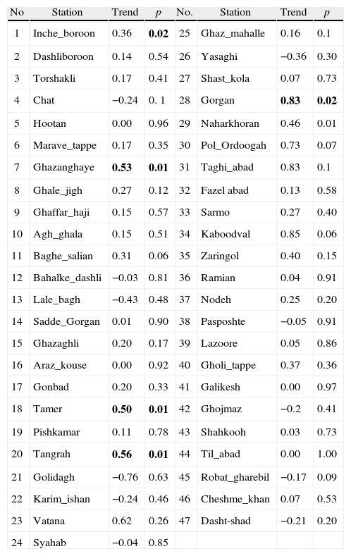
The results of the Mann-Kendall trend test are presented in Table III, from which it can be seen that out of 47 rainfall stations, only six stations demonstrate a statistically significant trend and the remaining 41 stations show no significant trend. As most observations of maximum daily rainfall in the study region do not have significant trends, it is reasonable to infer that the trends are not significant at the regional level and data can be treated as stationary series.

Table III.

Results of the trend analysis of maximum daily rainfall series using the Mann-Kendall test.

No	Station	Trend	p	No.	Station	Trend	p
1	Inche_boroon	0.36	0.02	25	Ghaz_mahalle	0.16	0.1
2	Dashliboroon	0.14	0.54	26	Yasaghi	−0.36	0.30
3	Torshakli	0.17	0.41	27	Shast_kola	0.07	0.73
4	Chat	−0.24	0. 1	28	Gorgan	0.83	0.02
5	Hootan	0.00	0.96	29	Naharkhoran	0.46	0.01
6	Marave_tappe	0.17	0.35	30	Pol_Ordoogah	0.73	0.07
7	Ghazanghaye	0.53	0.01	31	Taghi_abad	0.83	0.1
8	Ghale_jigh	0.27	0.12	32	Fazel abad	0.13	0.58
9	Ghaffar_haji	0.15	0.57	33	Sarmo	0.27	0.40
10	Agh_ghala	0.15	0.51	34	Kaboodval	0.85	0.06
11	Baghe_salian	0.31	0.06	35	Zaringol	0.40	0.15
12	Bahalke_dashli	−0.03	0.81	36	Ramian	0.04	0.91
13	Lale_bagh	−0.43	0.48	37	Nodeh	0.25	0.20
14	Sadde_Gorgan	0.01	0.90	38	Pasposhte	−0.05	0.91
15	Ghazaghli	0.20	0.17	39	Lazoore	0.05	0.86
16	Araz_kouse	0.00	0.92	40	Gholi_tappe	0.37	0.36
17	Gonbad	0.20	0.33	41	Galikesh	0.00	0.97
18	Tamer	0.50	0.01	42	Ghojmaz	−0.2	0.41
19	Pishkamar	0.11	0.78	43	Shahkooh	0.03	0.73
20	Tangrah	0.56	0.01	44	Til_abad	0.00	1.00
21	Golidagh	−0.76	0.63	45	Robat_gharebil	−0.17	0.09
22	Karim_ishan	−0.24	0.46	46	Cheshme_khan	0.07	0.53
23	Vatana	0.62	0.26	47	Dasht-shad	−0.21	0.20
24	Syahab	−0.04	0.85

Bold values denote the significant trends at a 0.95 significance level.

The values of the autocorrelation coefficients for lags 1 to 5 are plotted in the correlograms presented in Figure 2, where the dashed horizontal lines are intended to give critical values for testing whether or not the autocorrelation coefficients are significantly different from zero. It can be seen that for almost all stations autocorrelation coefficients are within the critical bounds, thus we might well consider the maximum daily rainfall series as time-independent.

Fig. 2.

Autocorrelation function analysis plots of maximum daily rainfall series for 45 rain gauge stations. Dashed lines indicate a 95% confidence interval.

The results of Moran’s I calculations suggested that cross-correlation among the stations was not statistically significant at the 5% significance level and the data series can be considered spatially independent.

3.2

Cluster analysis

As described in the methodology section, a hierarchical cluster analysis with Ward’s method was first applied to identify initial homogeneous regions. The two methods examined to help identifying an appropriate number of groups in the cluster analysis (i.e., silhouette widths and Mantel comparison), suggested a seven-region partitioning (Fig. 3). The result of Ward’s clustering with seven clusters is depicted in the dendrogram drawn in Figure 4.

Fig. 3.

Optimal number of clusters according to the silhouette widths and Mantel comparison method (the best partition is the one with the largest average silhouette width and the largest Pearson’s correlation). For further details refer to Borcard et al. (2011) and Rao and Srinivas (2008).

Fig. 4.

Dendrogram of clustered stations by the Ward’s method.

The rainfall clusters were reviewed to assess whether they are spatially continuous and physically reasonable. Inspection of the clusters, taking into account the physical/geographical conditions —particularly topography and proximity to the sea— showed that the derived rainfall groups and geographical conditions match each other very well, while differing rainfall clusters imply varying rainfall regimes. The spatial distribution of the rainfall groups is illustrated in Figure 5.

Fig. 5.

Location of sites in the seven relatively homogeneous clusters within the Golestan province.

The first region (group 1) includes the eight stations located in the arid and semi-arid northern parts of the province. The average altitude of the region is about 100 masl, and the mean annual precipitation is around 250 mm. The second homogenous region is formed by nine stations situated in the lowland plains in central parts of the province. This region has an average altitude of 23 masl and mean annual precipitation of 405 mm. The third group is comprised of six stations located in the lowland margins of the Caspian Sea and the surrounding plain areas with an average altitude of 33 masl and mean annual precipitation of 550 mm. Regions 1, 2 and 3 are low-elevation non-orographic areas. In these parts of the province, the Caspian Sea along with high pressure systems crossing the region play a great role in the temporal and spatial distribution of precipitation (Masoodian, 2008). High rainfalls in these regions are most likely caused by convective storms developing in the low-level moist air drawn westward from the Caspian Sea (Alijani, 1997). The fourth and fifth regions encompass the higher areas located on the northern slopes of the Alborz Mountains with an average altitude of 400 masl. Precipitation in these regions is influenced by orographic effects of the Alborz Mountains, which force westerly moist winds to rise. The amount of annual rainfall for regions 4 and 5 are 730 and 700 mm, respectively. Synoptic-scale cyclonic weather systems and associated fronts in combination with orographic effects provide the mechanisms for producing extreme rainfalls in these regions. The sixth homogeneous region includes four stations located in mountainous areas near the crest line of the Alborz Mountains but in the leeward southern face. Altitude of the region is above 1000 masl and mean annual precipitation is about 270 mm. Intense rainfalls in the region are produced predominately by winter storm events. The seventh region has only one station in the southwestern mountainous areas of the province with an altitude of 2240 masl and annual precipitation of 430 mm. What seems to differentiate this region from the others is the proximity of the mountains to the Caspian Sea. Precipitation characteristics of the region are influenced both by the presence of the mountains and the sea.

3.3

Discordancy, homogeneity, and goodness-of-fit tests

Using the R package lmomRFA, the homogeneity of the regions and the existence of any discordant station in each group were investigated. Accordingly, several subjective adjustments were made to refine the initial regions and reduce heterogeneity of the regions as measured by the heterogeneity measures H.

The result of the discordancy test indicated that four stations, namely Vatana (in region 3), Pishkamar (in region 4), Karim-Ishan (in region 4), and Dasht-shad (in region 6) were discordant with the other stations in their groups. These stations were deleted after it proved impossible to reassign them to other regions. Region 6, which had three stations, was merged with region 4 based on geographical and physical conditions. The combined region was homogeneous (H₁ = 0.01). Region 7, which contained only one station (Shahkooh), was also removed because assigning it to adjacent regions would cause them to be heterogeneous. After modification of the initial regions, the final number of regions was reduced to five, all of which were acceptably homogeneous (H₁ < 1) with no discordant stations as indicated in Table IV.

Table IV.

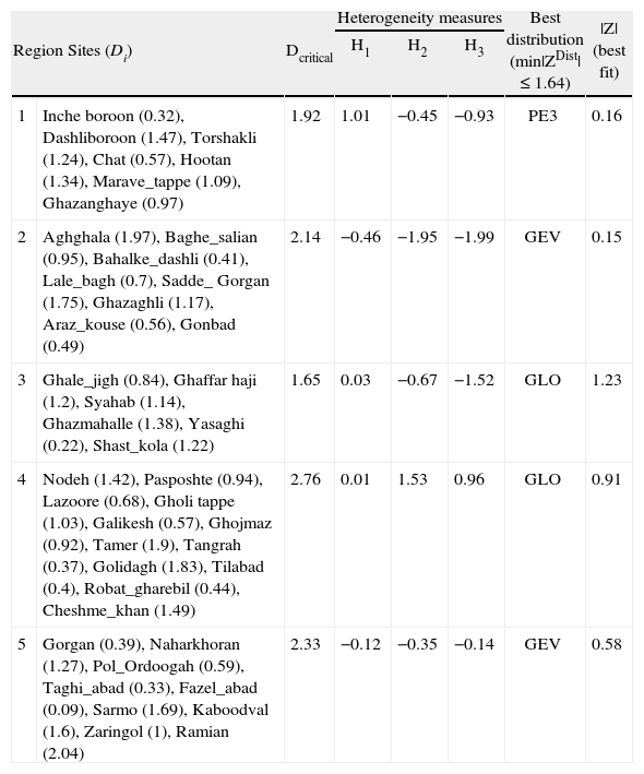
Discordance, heterogeneity and goodness-of-fit results for maximum daily rainfall series in five homogeneous regions.

Region Sites (Di)		Dcritical	Heterogeneity measures			Best distribution (min|Z^Dist|≤ 1.64)	|Z|(best fit)
			H1	H2	H3
1	Inche boroon (0.32), Dashliboroon (1.47), Torshakli (1.24), Chat (0.57), Hootan (1.34), Marave_tappe (1.09), Ghazanghaye (0.97)	1.92	1.01	−0.45	−0.93	PE3	0.16
2	Aghghala (1.97), Baghe_salian (0.95), Bahalke_dashli (0.41), Lale_bagh (0.7), Sadde_ Gorgan (1.75), Ghazaghli (1.17), Araz_kouse (0.56), Gonbad (0.49)	2.14	−0.46	−1.95	−1.99	GEV	0.15
3	Ghale_jigh (0.84), Ghaffar haji (1.2), Syahab (1.14), Ghazmahalle (1.38), Yasaghi (0.22), Shast_kola (1.22)	1.65	0.03	−0.67	−1.52	GLO	1.23
4	Nodeh (1.42), Pasposhte (0.94), Lazoore (0.68), Gholi tappe (1.03), Galikesh (0.57), Ghojmaz (0.92), Tamer (1.9), Tangrah (0.37), Golidagh (1.83), Tilabad (0.4), Robat_gharebil (0.44), Cheshme_khan (1.49)	2.76	0.01	1.53	0.96	GLO	0.91
5	Gorgan (0.39), Naharkhoran (1.27), Pol_Ordoogah (0.59), Taghi_abad (0.33), Fazel_abad (0.09), Sarmo (1.69), Kaboodval (1.6), Zaringol (1), Ramian (2.04)	2.33	−0.12	−0.35	−0.14	GEV	0.58

For making a decision about the parent distribution for each homogeneous region, the goodness-of-fit statistic Z^Dist of various candidate distributions, including generalized logistic (GLO), generalized extreme-value (GEV), generalized normal (GNO), generalized pareto (GPA), and Pearson type III (PE3), was computed. The best distribution for each homogeneous region according to Z^Dist is presented in Table IV. For illustrative purposes, the L-moment ratio diagrams showing the location of the regional average L-moments with theoretical L-skewness/L-kurtosis relationships for the different candidate distributions, are presented in Figure 6.

Fig. 6.

L-moment ratio diagrams for maximum daily rainfall series at five homogeneous regions The bold asterisks show the regional weighted average of L-Cs versus L-Ck.

For region 1, the PE3 distribution is identified as the best distribution. The GEV has the best goodness-of-fit for data in regions 2 and 5, and the GLO distribution is best fitted for regions 3 and 4. The results do not suggest any parent frequency distribution function for the entire region, mainly due to the complexity of rainfall generating mechanisms resulting from the combined effects of local rainfall factors such as elevation and topography with large atmospheric systems.

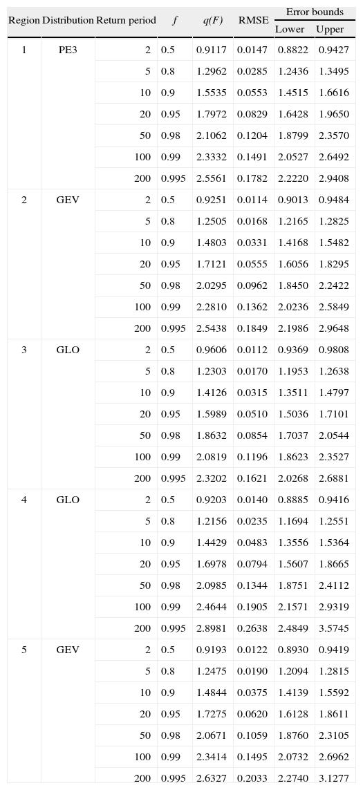
3.4

Design rainfall depth estimation through index-rainfall approach

For each homogeneous region, the best-fit distribution of regional data was used for estimating dimensionless regional frequency distribution (regional growth curve). The bias, RMSE, and 90% error bounds of the estimated growth curves were calculated through the Monte Carlo simulation procedure. The results are given in Table V and Figure 7. It is evident from the Figures that uncertainty of the regional quantiles increases with the return period. The RMSE values of the estimated growth curves for five homogeneous regions range from 0.011 to 0.19 when return periods of rainfall extremes are less than 100 years. However, high RMSE values and error bounds are noted in the upper tail, suggesting the unreliability of quantiles with return period T > 100 years.

Table V.

Regional quantiles and accuracy measures for the five homogeneous regions.

Region	Distribution	Return period	f	q(F)	RMSE	Error bounds
						Lower	Upper
1	PE3	2	0.5	0.9117	0.0147	0.8822	0.9427
		5	0.8	1.2962	0.0285	1.2436	1.3495
		10	0.9	1.5535	0.0553	1.4515	1.6616
		20	0.95	1.7972	0.0829	1.6428	1.9650
		50	0.98	2.1062	0.1204	1.8799	2.3570
		100	0.99	2.3332	0.1491	2.0527	2.6492
		200	0.995	2.5561	0.1782	2.2220	2.9408
2	GEV	2	0.5	0.9251	0.0114	0.9013	0.9484
		5	0.8	1.2505	0.0168	1.2165	1.2825
		10	0.9	1.4803	0.0331	1.4168	1.5482
		20	0.95	1.7121	0.0555	1.6056	1.8295
		50	0.98	2.0295	0.0962	1.8450	2.2422
		100	0.99	2.2810	0.1362	2.0236	2.5849
		200	0.995	2.5438	0.1849	2.1986	2.9648
3	GLO	2	0.5	0.9606	0.0112	0.9369	0.9808
		5	0.8	1.2303	0.0170	1.1953	1.2638
		10	0.9	1.4126	0.0315	1.3511	1.4797
		20	0.95	1.5989	0.0510	1.5036	1.7101
		50	0.98	1.8632	0.0854	1.7037	2.0544
		100	0.99	2.0819	0.1196	1.8623	2.3527
		200	0.995	2.3202	0.1621	2.0268	2.6881
4	GLO	2	0.5	0.9203	0.0140	0.8885	0.9416
		5	0.8	1.2156	0.0235	1.1694	1.2551
		10	0.9	1.4429	0.0483	1.3556	1.5364
		20	0.95	1.6978	0.0794	1.5607	1.8665
		50	0.98	2.0985	0.1344	1.8751	2.4112
		100	0.99	2.4644	0.1905	2.1571	2.9319
		200	0.995	2.8981	0.2638	2.4849	3.5745
5	GEV	2	0.5	0.9193	0.0122	0.8930	0.9419
		5	0.8	1.2475	0.0190	1.2094	1.2815
		10	0.9	1.4844	0.0375	1.4139	1.5592
		20	0.95	1.7275	0.0620	1.6128	1.8611
		50	0.98	2.0671	0.1059	1.8760	2.3105
		100	0.99	2.3414	0.1495	2.0732	2.6962
		200	0.995	2.6327	0.2033	2.2740	3.1277

fig. 7.

Estimated regional growth curves, with 90% error bounds for the five homogeneous regions.

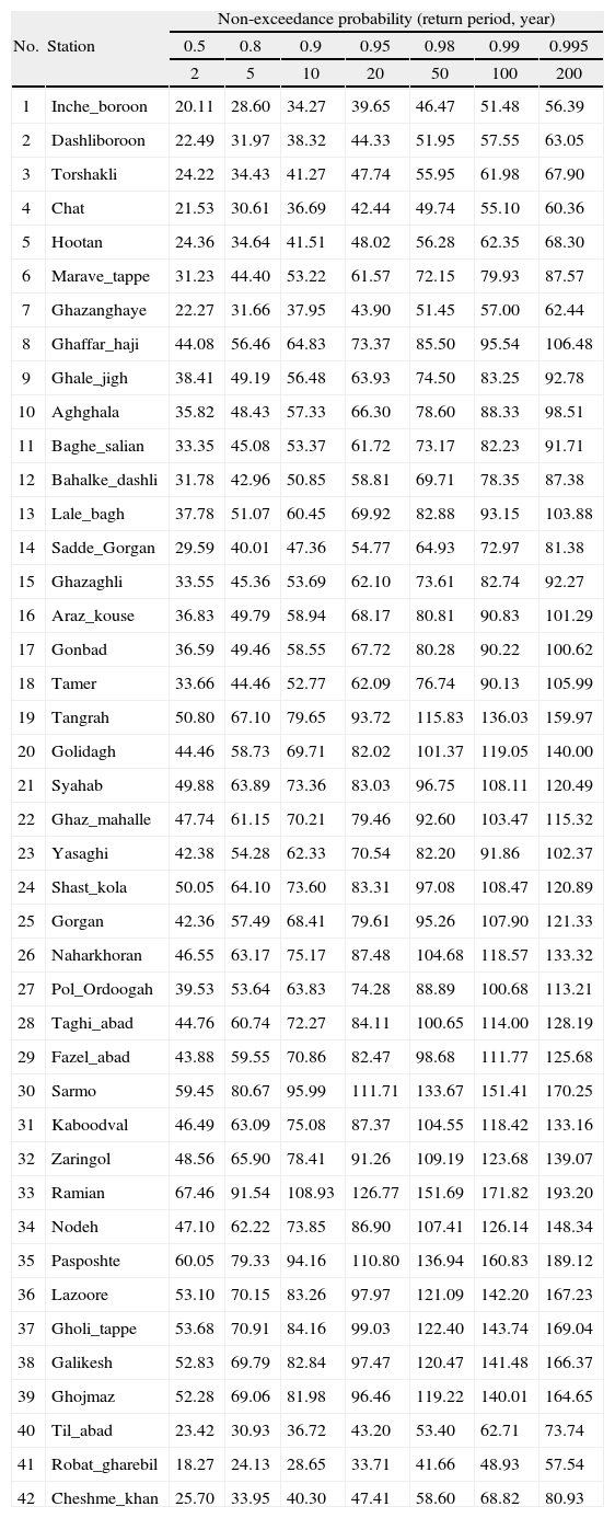
At-site 24-h design rainfall depths for different year return periods were then obtained by scaling the regional growth curve by the sites’ average annual maximum rainfall. Table VI presents quantile estimations for each rain-gauge station.

Table VI.

Estimated máximum daily rainfalls corresponding to different non-exceedance probabilities (return periods) in the Golestan province using L-moment regional frequency analysis.

No.	Station	Non-exceedance probability (return period, year)
		0.5	0.8	0.9	0.95	0.98	0.99	0.995
		2	5	10	20	50	100	200
1	Inche_boroon	20.11	28.60	34.27	39.65	46.47	51.48	56.39
2	Dashliboroon	22.49	31.97	38.32	44.33	51.95	57.55	63.05
3	Torshakli	24.22	34.43	41.27	47.74	55.95	61.98	67.90
4	Chat	21.53	30.61	36.69	42.44	49.74	55.10	60.36
5	Hootan	24.36	34.64	41.51	48.02	56.28	62.35	68.30
6	Marave_tappe	31.23	44.40	53.22	61.57	72.15	79.93	87.57
7	Ghazanghaye	22.27	31.66	37.95	43.90	51.45	57.00	62.44
8	Ghaffar_haji	44.08	56.46	64.83	73.37	85.50	95.54	106.48
9	Ghale_jigh	38.41	49.19	56.48	63.93	74.50	83.25	92.78
10	Aghghala	35.82	48.43	57.33	66.30	78.60	88.33	98.51
11	Baghe_salian	33.35	45.08	53.37	61.72	73.17	82.23	91.71
12	Bahalke_dashli	31.78	42.96	50.85	58.81	69.71	78.35	87.38
13	Lale_bagh	37.78	51.07	60.45	69.92	82.88	93.15	103.88
14	Sadde_Gorgan	29.59	40.01	47.36	54.77	64.93	72.97	81.38
15	Ghazaghli	33.55	45.36	53.69	62.10	73.61	82.74	92.27
16	Araz_kouse	36.83	49.79	58.94	68.17	80.81	90.83	101.29
17	Gonbad	36.59	49.46	58.55	67.72	80.28	90.22	100.62
18	Tamer	33.66	44.46	52.77	62.09	76.74	90.13	105.99
19	Tangrah	50.80	67.10	79.65	93.72	115.83	136.03	159.97
20	Golidagh	44.46	58.73	69.71	82.02	101.37	119.05	140.00
21	Syahab	49.88	63.89	73.36	83.03	96.75	108.11	120.49
22	Ghaz_mahalle	47.74	61.15	70.21	79.46	92.60	103.47	115.32
23	Yasaghi	42.38	54.28	62.33	70.54	82.20	91.86	102.37
24	Shast_kola	50.05	64.10	73.60	83.31	97.08	108.47	120.89
25	Gorgan	42.36	57.49	68.41	79.61	95.26	107.90	121.33
26	Naharkhoran	46.55	63.17	75.17	87.48	104.68	118.57	133.32
27	Pol_Ordoogah	39.53	53.64	63.83	74.28	88.89	100.68	113.21
28	Taghi_abad	44.76	60.74	72.27	84.11	100.65	114.00	128.19
29	Fazel_abad	43.88	59.55	70.86	82.47	98.68	111.77	125.68
30	Sarmo	59.45	80.67	95.99	111.71	133.67	151.41	170.25
31	Kaboodval	46.49	63.09	75.08	87.37	104.55	118.42	133.16
32	Zaringol	48.56	65.90	78.41	91.26	109.19	123.68	139.07
33	Ramian	67.46	91.54	108.93	126.77	151.69	171.82	193.20
34	Nodeh	47.10	62.22	73.85	86.90	107.41	126.14	148.34
35	Pasposhte	60.05	79.33	94.16	110.80	136.94	160.83	189.12
36	Lazoore	53.10	70.15	83.26	97.97	121.09	142.20	167.23
37	Gholi_tappe	53.68	70.91	84.16	99.03	122.40	143.74	169.04
38	Galikesh	52.83	69.79	82.84	97.47	120.47	141.48	166.37
39	Ghojmaz	52.28	69.06	81.98	96.46	119.22	140.01	164.65
40	Til_abad	23.42	30.93	36.72	43.20	53.40	62.71	73.74
41	Robat_gharebil	18.27	24.13	28.65	33.71	41.66	48.93	57.54
42	Cheshme_khan	25.70	33.95	40.30	47.41	58.60	68.82	80.93

The procedure for estimating rainfall quantiles at ungauged sites is similar to that for gauged sites except that an estimate of the at-site average maximum rainfall (l₁) must be obtained from other sources or other methods. Investigations revealed that there is a strong relationship between l₁ and mean annual precipitation in the Golestan province (Fig. 8). The following equation was developed to estimate l₁ values at ungauged sites in Golestan:

where l₁ is the average annual maximum rainfall (mm) and MAP is the mean annual precipitation (mm).

Fig. 8.

Relationship between at-site average maximum rainfall and mean annual precipitation in the Golestan province.

Isopluvial precipitation maps of the province generated using interpolation methods (Zare Garizi et al., 2013), in conjunction with Eq. (7) can provide a basis for estimating index rainfall for the entire province. Design rainfall depths at ungauged sites can then be estimated using the index rainfall and the regional growth curves.

4

Conclusions

In the present study, regional frequency analysis of maximum daily rainfalls was investigated for the Golestan province located in northeastern Iran. Being one of the major disaster-prone regions of Iran, the Golestan province includes areas affected by exceptional flash flood events caused by extreme rainfalls. The most recent examples are two events that occurred in 2001 and 2002, which caused significant damages to human life and property. With this in mind, the present study intended to find appropriate regional frequency distributions for maximum daily rainfalls and predict the return values of extreme rain-fall events (design rainfall depths). L-moment regionalization procedures coupled with an index rainfall method were applied to maximum rainfall records of 47 stations across Golestan.

Due to the complex geographic and hydro-climatological characteristics of the region, an important research issue focused on breaking down the large area into homogeneous and coherent sub-regions. The area of the Golestan province was divided into five homogeneous regions, based on the cluster analysis of site characteristics and tests for regional homogeneity. The site characteristics utilized in this study enabled relatively homogeneous regions of extreme rainfall within Golestan to be easily identified, with minor subjective interventions. Nevertheless, followed by the recommendation by Kyselý et al. (2007) it should be noted that, since the regions configured are not only homogeneous as to the statistical characteristics of extreme rainfalls, but also reflect climatological differences in precipitation regimes and synoptic patterns causing heavy precipitation, their future application may not be limited to the frequency analysis of extremes.

The goodness-of-fit results indicated that the best fitting distribution is different for individual homogeneous regions. The difference may be a result of distinctive climatic and geographic conditions. Further researches using a larger database could be carried out to prove the effect of geographic conditions and rainfall regimes on the type of maximum rain-fall distribution functions. The estimated regional quantiles and their accuracy measures produced by Monte Carlo simulations demonstrate that the estimation uncertainty as measured by the RMSE values and 90% error bounds is relatively low when return periods are less than 100 years. But, for higher return periods, rainfall estimates should be treated with caution. More station years, either from longer records or more stations in the regions, would be required for rainfall estimates above T = 100 years. It was found from the analyses that index rainfall (at-site average maximum rainfall) can be estimated reasonably well as a function of mean annual precipitation in the Golestan province. Index rainfalls combined with the regional growth curves, can be used to estimate design rainfalls at ungauged sites.

Overall, it was found that cluster analysis together with the L-moments based regional frequency analysis technique can be applied successfully in deriving design rainfall estimates for northeastern Iran. The approach utilized in this study and the findings are of great scientific and practical merit, particularly for the purpose of planning for weather-related emergencies and design of hydraulic engineering structures.

Acknowledgments

The authors would like to thank the Golestan Province Regional Water Agency for providing necessary data for the study.