


El uso de datos del flujo de energía para validar modelos de superficie requiere que se satisfaga el cierre del balance de energía; sin embargo, esta condición no suele verificarse cuando la energía disponible es mayor que la suma de los flujos turbulentos verticales. Este trabajo presenta una evaluación de los problemas relacionados con el cierre del balance de energía. Los datos evaluados corresponden a una base de datos de 2012 de Livraga, Italia, obtenidos en una estación micrometeorológica de covarianza eddy localizada en un campo de maíz del valle del Po. El cierre del balance de energía se calcula mediante la regresión estadística de flujos turbulentos de energía y flujos de calor en el suelo. Por lo general, los resultados indican ausencia de cierre con un desequilibrio medio del orden de 20%. Las condiciones del almacenaje son la razón fundamental de la ausencia de cierre del balance, pero las condiciones de mezcla de flujos turbulentos también desempeñan un papel importante en las estimaciones confiables de estos flujos. Recientemente se ha introducido en la literatura el estudio del balance de energía, como un problema de escala. Aquí se ha analizado un área de origen representativa para cada flujo de energía que interviene en el balance, y el cierre se ha realizado en función de las áreas con huellas de flujos turbulentos. También se han estudiado los efectos de la heterogeneidad de la superficie y la estacionalidad para comprender la influencia del crecimiento de la cubierta vegetal en el cierre del balance de energía. Se han utilizado datos de alta frecuencia para calcular funciones coespectrales y de ojiva, los cuales sugieren que un periodo medio de 30min puede perder las escalas temporales que contribuyen a la existencia de flujos turbulentos. Por último, se calculan las estimaciones de errores aleatorios de calor sensible para proporcionar información sobre deficiencias en el sistema de medición y el transporte turbulento.
The use of energy fluxes data to validate land surface models requires that energy balance closure conservation is satisfied, but usually this condition is not verified when the available energy is bigger than the sum of turbulent vertical fluxes. In this work, a comprehensive evaluation of energy balance closure problems is performed on a 2012 data set from Livraga obtained by a micrometeorological eddy covariance station located in a maize field in the Po Valley. Energy balance closure is calculated by statistical regression of turbulent energy fluxes and soil heat flux against available energy. Generally, the results indicate a lack of closure with a mean imbalance in the order of 20%. Storage terms are the main reason for the unclosed energy balance but also the turbulent mixing conditions play a fundamental role in reliable turbulent flux estimations. Recently introduced in literature, the energy balance problem has been studied as a scale problem. A representative source area for each flux of the energy balance has been analyzed and the closure has been performed in function of turbulent flux footprint areas. Surface heterogeneity and seasonality effects have been studied to understand the influence of canopy growth on the energy balance closure. High frequency data have been used to calculate co-spectral and ogive functions, which suggest that an averaging period of 30min may miss temporal scales that contribute to the turbulent fluxes. Finally, latent and sensible heat random error estimations are computed to give information about the measurement system and turbulence transport deficiencies.
Surface energy fluxes are important for a huge range of applications over different spatial and temporal scales: from flash flood simulations at a basin scale to water management in agricultural areas. Thus, it is important to understand the quality of measured fluxes before using them for land-atmosphere simulations.
The quality of eddy covariance measurements is influenced not only by possible deviations from the theoretical assumptions but also by problems of sensor configurations and meteorological conditions (Foken and Wichura, 1996). However, it is difficult to isolate the causes of measurement errors. Instrumental errors, uncorrected sensor configurations, problems of heterogeneities in the area and atmospheric conditions are the main problems that affect data quality (Wilson et al., 2002; Foken et al., 2006; Foken, 2008a; Jacobs et al., 2008). The eddy covariance method produces reliable results when the theoretical assumptions in the surface layer are satisfied (Foken and Wichura, 1996; Baldocchi et al., 2001; Fisher et al., 2007). In particular, theoretical requirements such as steady-state conditions, horizontal homogeneity of the field, validity of the mass conservation equation, negligible vertical density flux, turbulent fluxes constant with height, and flat topography, should be satisfied. Moreover, the sensors configuration should be analyzed in relation to the sampling duration and frequency, separation of the sonic anemometer and gas analyzer, and sensor placement within the constant flux layer (but out of the roughness sub-layer). Meteorological conditions such as precipitation events and low turbulence, especially at nighttime, can lead to errors in fluxes measurements.
The unbalance of the energy budget has been widely studied in the last decade due to the fact that the use of energy fluxes to validate land surface models requires the closure of the energy balance to be satisfied. The energy budget is typically not closed when energy fluxes are measured with an eddy covariance (EC) station and the available energy is bigger than the sum of turbulent vertical heat fluxes within a ratio of 70-90% (Wilson et al., 2002; Foken et al., 2006; Jacobs et al., 2008; Ma et al., 2009). Thus, it is important to understand the different factors that can lead to an improvement of the energy balance closure.
The first cause of the lack of energy balance closure is linked to an incorrect implementation of a complete set of instrumental and flux corrections as described in Aubinet et al. (2000). Axis rotation, spike removal, time lag compensation and detrending are the preliminary correction processes which should be applied on high frequency raw data sets measured by a sonic anemometer and a gas analyzer. Subsequently, spectral information losses, air density fluctuations and humidity effects have to be taken into account to obtain reliable fluxes of latent and sensible heat (Webb et al., 1980; Moncrieff et al., 1997; Van Dijk et al., 2003).
However, later studies discuss the unbalance problem as an effect of the fractional coverage of vegetation and the influence of soil storage (Foken, 2008b). Additional storage terms, like the ones linked to photosynthesis processes or vegetation canopy, give a relevant improvement in energy balance closure (Meyers and Hollinger, 2004).
Different time aggregation could reduce the effect of storage terms because they have an opposite behavior during daytime and nighttime (Papale et al., 2006). Some recent works (Oncley et al., 1993; Finnigan et al., 2003) suggest that the averaged time (generally 30min) chosen to calculate covariances could be inadequate for assessing turbulent fluxes. An ogive function for each half hour data set can be a good indicator of measurement errors associated to such energy balance problems (Oncley et al., 1993).
Moreover, the energy balance closure can be seen as a scale problem, because the representativeness of a measured flux is a scale function (Masseroni et al., 2012). Usually, for homogeneous areas, the assumption that source areas are the same for all fluxes is considered valid. However, these areas can be significantly different if the footprint of turbulent fluxes is compared to the source area of ground heat flux. So, a portion of the error in energy balance closure can be related to the difficulty of matching the footprint area of eddy covariance fluxes with the source areas of the instruments that measure net radiation and ground heat flux (Schmid, 1997; Hsieh et al., 2000; Wilson et al., 2002).
Eddy flux measurements can be underestimated during periods with low turbulence and air mixing. This underestimation acts as a selective systematic error and it generally occurs during nighttime. Massman and Lee (2002) listed the possible causes of this nighttime flux error. There is now a large consensus recognizing that the most probable cause of error is the presence of small-scale movements associated with drainage flows or land breezes that take place in low turbulence conditions and provoke a decoupling between the soil surface and the canopy top. In these conditions, advection becomes an important term in the flux balance and cannot be neglected anymore. It has been recently suggested (Finnigan et al., 2006) that, contrary to what was thought before, advection probably affects most of the sites, including flat and homogeneous ones. Direct advection fluxes are difficult to measure as they require several measurement towers at the same site. Notable attempts were made by Aubinet et al. (2003), Feigenwinter et al. (2004), Staebler and Fitzjarrald (2004) and Marcolla et al. (2005), who found that advection fluxes are usually significant during calm weather conditions. However, in most cases, the measurement uncertainty is too large to allow a precise estimation. In addition, such direct measurements require an extremely complicated setup to allow routine measurements at each site. In practice, the flux problem is bypassed by discarding the data corresponding to low mixing periods. The friction velocity is currently used as a criterion to discriminate between low and high mixing periods. This approach is generally known as the “u* correction”. Although being currently the best and most widely used method to avoid the problem, the u* correction is affected by several drawbacks and must be applied carfully.
Factors connected with growing vegetation and seasonality have been investigated. As shown in Panin et al. (1998), the unbalance could be attributed to the influence of surface heterogeneity and vegetation height with respect to the sensors position.
Different sources of uncertainties in flux measurements can be sometimes difficult to assess. Random measurement errors in flux data, including errors due to the measurement system and turbulence transport, have been assessed by Hollinger and Richardson (2005), comparing the measurements from two towers with the same flux source area (“footprint”); and by Richardson et al. (2006), comparing pairs of measurements made on two successive days from the same tower under equivalent environmental conditions. A simple method described in Moncrieff et al. (1996) can be used to quantify the influence of random errors on momentum and latent and sensible heat, calculating a degree of uncertainty for each turbulent flux.
In this work, relevant findings on the energy balance closure problem over a maize field in the Po Valley are summarized mainly on the basis of recent investigation works, such as those by Wilson et al. (2002), Oncley et al. (2007) and Foken (2008b). Turbulent fluxes from a raw data set of high frequency measurements, are obtained using the Eddy Pro 4.0 software with the main objective of standardizing the correction procedure of eddy covariance measurements. The impact of each investigated factor is quantified by the slope and intercept values between turbulent vertical heat fluxes (latent heat, sensible heat and ground heat fluxes) and available energy (net radiation) from a regression analysis on a half hourly basis. Each examined factor is studied separately to improve the understanding of its impact on the energy balance closure. Theoretical backgrounds are not summarized in a separate chapter, but they are included in each sub-paragraph to improve the description of the exanimated problems. Only practical formulas are shown, while mathematical approaches are quoted in literature.
2Instruments, data collection and site descriptionThe experimental campaign was carried out over a maize field at Livraga (LO) in the Po Valley during the year 2012. The field is about 10 hectares long (Fig. 1 ) and the local overall topography is flat. In the middle of the field an island of about 50 m2 is designed to include agro-micrometeorological instruments and devices.

Eddy covariance data are measured by a tridimensional sonic anemometer (Young 81000, Campbell Scientific) and an open path gas analyzer (LI 7500 by LICOR Industry) located at the top of a tower approximately 5m above the ground. High frequency (20Hz) measurements are stored in a compact flash of 2Gb connected to the data logger CR5000 (Campbell Scientific) and downloaded in situ weekly. Only three wind velocity components: sonic temperature, vapor and carbon dioxide concentrations (raw data) are stored in the compact flash. Simultaneously, net radiation —measured by a radiometer (CNR1 by Kipp & Zonen) at a height of 4.5m—, soil heat flux —measured with a flux plate (HFP01 by Campbell Scientific) at a depth of 6cm from the ground and tested according to the Masseroni et al. (2013a) method— and soil temperature —measured by two thermocouples at a depth of 4 and 8cm from the ground— are stored on the data logger in different memory tables. Soil moisture (detected by a CS 616 probe by Campbell Scientific) at different levels (10, 30 and 50cm) and rain are also measured in the island. Averaged fluxes are calculated over a time step of 30min.
Experimental measurements were carried out from May 21 to September 7, but the dataset is composed only by 3103 averaged data, because some gaps due to malfunctioning of the instruments or rainfall days are shown in the data sequences. From the Julian days 131 to 241 of the the field is covered by vegetation, while the remaining days of the year it is characterized by bare soil. Vegetation height varies from 0 to 320cm and the canopy growth throughout the project can be spatially considered homogeneous across the field.
Wind direction, generally from the west during daytime and from the east during nighttime, is quite steady, but some days it is strongly variable. Considering each wind direction, the eddy tower position is compatible with the constant flux layer (CFL) (Elliot, 1958). CFL is defined as 10 to 15% of the internal boundary layer (Baldocchi and Rao, 1995), and it represents a space area where measured fluxes by the eddy tower are constant. Applying Elliot’s (1958) formula in unfavourable conditions of bare soil, with a calculated aerodynamic roughness of about 0.04m (Garratt, 1993), the CFL depth at the tower is about 6 m, ensuring that the eddy covariance instruments (tridimensional sonic anemometer and gas analyser) remain within the CFL.
During the summer period the site is typically characterized by a cloud-free sky in association with high latent heat flux and net radiation values of about 600 and 700 Wm-2, respectively. Cumulated rain over the experimental period is about 200mm, while soil moisture measured at a depth of 10cm varies between maximum and minimum peaks of about 0.4 and 0.15, respectively.
3The energy balance closure problemEnergy balance closure, a formulation of the first law of thermodynamics, requires that the sum of latent heat (LE), sensible heat (H) and ground heat flux (G) is equal to all other energy sinks or sources (Eq. 1).
where Rn is the net radiation. Generally, fluxes are typically integrated over 30-min periods, thus building the basis to calculate energy balance on annual time scales. The slope (given by LE+H+GRn−1) and intercept values of the regression line quantify the reliability of the energy balance closure, which is close to 1 in an ideal case. In the following sections, relevant findings on the energy balance closure are summarized and data processing results using the experimental measurements are shown.3.1Effects of data correction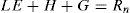
In this sub-section, the procedures necessary to obtain reliable fluxes starting from high frequency raw data set are briefly described (Corbari et al., 2012).
Eddy covariance measurements have to be corrected to obtain reliable turbulent fluxes of latent and sensible heat. Before calculating fluxes, two groups of corrections should be implemented: “instrumental” and “physical” corrections.
Instrumental corrections can be considered as preliminary processes that have to be directly applied on high frequency measurements to prepare the data set for fluxes calculation.
3.1.1Axis rotation for tilt correctionTilt correction algorithms are necessary to correct wind statistics for any misalignment of the sonic anemometer with respect to the local wind streamlines. Wilczak et al. (2001) propose three typologies of correction algorithms, and for the Livraga 2012 dataset a double rotation method was used. With this method the anemometer tilt is compensated by rotating raw wind components to nullify the average cross-stream and vertical wind components.
3.1.2Spike removalThe so-called despiking procedure consists in detecting and eliminating short term outranged values in the time series. Following Vickers and Mahrt (1997), a spike is represented by a single consecutive value (or a maximum of three consecutive values) that is outside the plausible range defined within a certain time window that moves throughout the time series.
3.1.3Time lag compensationIn an open path system the time lag between anemometric variables and variables measured by a gas analyzer is due to the physical distance between the two instruments, which are usually placed several decimeters (or less) apart to avoid mutual disturbances. The wind field takes some time to travel between both instruments, which results in a certain delay between the sampling of the same air parcel by each one of the two instruments (Runkle et al., 2012).
3.1.4DetrendingThe eddy correlation method for calculating fluxes requires that the fluctuating components of the measured signals are derived by subtracting them from the mean signals. In steady-state conditions simple linear means would be adequate, but steady state conditions rarely exist in the atmosphere and it is necessary to remove the long-term trends in the data which do not contribute to the flux (Gash and Culf, 1996).
After completing the preliminary processes, physical corrections have to be implemented. Spectral information losses, air density fluctuations and humidity effects on sonic temperature are taken into account in accordance with the procedure described in Ueyama et al. (2012).
3.1.5Spectral correctionSpectral corrections compensate flux underestimations derived from two distinct effects. The first effect is referred to fluxes that are calculated on a finite averaging time, implying that longer-term turbulent contributions are under-sampled at some extent, or completely. The correction of these flux losses is referred to as “high-pass filtering” because the detrending method acts similarly to a high-pass filter, attenuating flux contributions in the frequency range close to the flux-averaging interval. The second effect is related to instrumental and setup limitations that do not allow sampling of the full spatiotemporal turbulence fluctuations and necessarily imply some space or time averaging of smaller eddies, as well as actual dampening of the small-scale turbulent fluctuations (Moncrieff et al., 1997; Masseroni et al., 2013b).
3.1.6WPL correctionThe open-path gas analyzer does not measure non-dimensional carbon dioxide and water vapor concentrations as mixing ratios, but it does measure carbon dioxide and water vapor densities. For this reason, the trace gas flux that is measured by this analyzer needs to be corrected for the mean vertical flow due to air density fluctuation. Webb et al. (1980) suggested that the flux due to the mean vertical flow cannot be neglected for trace gases such as water vapor and carbon dioxide. To evaluate the magnitude of the influence exerted by the mean vertical flow, Webb et al. (1980) assumed that the vertical flux of dry air should be zero. Practically, sensible and latent heat fluxes evaluated by the eddy covariance technique are used to calculate water vapor and carbon dioxide fluxes by the mean vertical flow (WPL correction).
3.1.7VD correctionThe sonic anemometer measures wind velocity components and sonic temperature. Sonic temperature, which is the basis of the sensible heat calculation, is affected both by humidity and velocity fluctuations. Van Dijk et al. (2003), revising the experiment carried out by Schotanus et al. (1983), define a correction term to be applied on the sensible heat formula in order to obtain a reliable flux (VD correction).
The impact of corrections on turbulent fluxes, as a consequence of the procedure described above, can be founded in the work of Ueyama et al. (2012). As shown in Figure 2, where the ensemble means of diurnal variations of turbulent fluxes over the whole experimental period are computed, if correction procedures are not applied (Fig. 2a), latent, sensible and ground heat fluxes collapse to zero during daytime, while in nighttime, overestimations of latent and sensible heat produce unsatisfactory flux interpretations. Instead, if correction procedures are applied (Fig. 2b), the fluxes partitioning is quite similar to that shown in many literature works.
 Uncorrected fluxes. (b) Corrected fluxes.")
The energy balance closure calculated after correction procedures were applied only on latent and sensible heat fluxes is 0.75, with a correlation coefficient (R2) of about 0.8 and an intercept of about 10 Wm-2.
3.2Effect of the storage termsEddy covariance measurements are based on turbulent air mixing and vertical flux exchanges. Sometimes, a portion of latent and sensible heat is stored below the measurement point, and these concentrations are not measured by the anemometer and gas analyzer. Usually, when canopy covers the field, the effect of its heat storage and photosynthesis flux increase drastically, reaching a value of about 10% of net radiation (Meyers and Hollinger, 2004). The best way to compute the storage flux is by deducing it from a concentration profile method inside the canopy (Papale et al., 2006). However, a discrete estimation based only on concentrations at the tower top is used on many sites (Meyers and Hollinger, 2004). Moreover, a correction is required to account for the heat storage that occurs in the layer between the soil surface and the heat flux plate (Mayocchi and Bristow, 1995). Thus, Eq. (1) can be rewritten with the addition of the storage terms (Eq. 2).
where Sp is the energy flux for photosynthesis, Sc is the canopy heat storage in biomass and water content and Sg is the ground heat storage above the soil heat plate.
Latent and sensible heat fluxes are computed and all corrections described in Ueyama et al. (2012) are applied. Net radiation is directly measured with the radiometer, while G is performed using the measurements obtained with the heat flux plate and thermocouples, applying the method quoted in Kustas et al. (2000).
The heat storage terms for the local surface energy balance are calculated by computing the total enthalpy change over a given time interval (Δt), which is 30min. For the canopy, the rate change in enthalpy is described by Eq. (3).
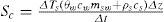
where Δta is the temperature exchange over the canopy directly measured by a radiometer. Plant water mass (mw), biomass (mb) density, specific heat for plant water (cw) and biomass (cb) were directly estimated by Meyers and Hollinger (2004), who weighed, dried, and weighed the maize plant again in order to assess its water content and biomass density. A similar procedure for heat storage in the soil surface is followed (Eq. 4).where Δts is the temperature exchange in the soil, msw is the density of water, θw is the measured volumetric content measured with a soil moisture probe at a 10cm depth, Δz is the depth above the soil heat plate up to the ground surface, ρs is the soil bulk density, and cs is the specific heat capacity of soil (Kustas and Daughtry, 1990).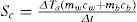
The light energy transformed in the photosynthetic process to carbon bond energy in the biomass has long been ignored when compared to other terms in the surface energy balance. However, as the lack of closure in surface energy balance continues intriguing researchers (Meyers and Hollinger, 2004), all of the data processing methods and terms should be reevaluated.
Analyzing the formation of glucose in its chemical reaction (Eq. 5), an estimate of the energy used in photosynthesis is obtained from the net sum of energy required to break the bonds of the reactants and those in the generation of glucose and oxygen.

This is the solar energy, which is now stored in the bonds of carbohydrate. It is ≈ 422 kJ per mole of CO2 fixed by photosynthesis (Nobel, 1974). A canopy assimilation rate of 2.5 mg CO2 m-2 s-1equates to an energy flux of 28 Wm-2. This conversion factor is used to compute the measured photosynthesis rates from the eddy covariance measurements to an equivalent energy flux.
In accordance with the Meyers and Hollinger (2004) procedure, storage terms are computed for the daytime period only, and data are grouped into 2-h bins beginning at 6:00 a.m. and ending at 18:00 p.m. The averaged daytime storage fluxes for the whole experimental period are presented in Figure 3.Figure 3a shows that the heat storage in the soil is greater than the other storage fluxes. Its trend is characterized by a peak of about 34 Wm-2 in correspondence with midday. During the morning, heat storage in the soil increases while in the afternoon it decreases down to 10 Wm-2. The photosynthesis storage term has a similar behavior, with a peak of about 10 Wm-2, while the canopy heat storage term tends to decrease during the day. Figure 3b shows the ratio between the sum of storage terms (total storage) and net radiation, which represents the available energy in the ecosystem. The storage fluxes constitute a significant fraction of the available energy with a ratio of about 10%, which is quite constant from 8:00 a.m. to 14:00 p.m., while it tends to decrease in the late afternoon.
 Average daytime cycle for each storage term for the whole experimental period. (b) Fraction of net radiation that is portioned to storage for maize plants.")
The effect of storage terms on the surface energy balance is examined by comparing the sum of H, LE and G with and without each storage flux, against Rn for the daytime periods over the whole experimental campaign. For the maize filed, without including the storage terms, the slope from a simple linear regression is 0.75 with an R2 of about 0.8 (Fig. 4). When the storage terms in the surface energy balance are included, the slope of the linear regression tends to increase up to 0.86 with an R2 of about 0.8 and an intercept of about 1.8 Wm-2. If closure storage terms are included in the energy balance, the systematic error in fluxes, described by linear regression intercept, is characterized by a drastic decreasing from 10 to 1.8 Wm-2. As explained in Foken (2008a), the ground heat storage has to be added to soil heat flux in order to obtain reliable G flux estimations. In fact, as shown in Figure 4, the ground storage term plays a fundament role in the energy balance closure improvement, having a positive influence of about 6%, which is equal to about 54% of the total energy balance improvement when considering the whole storage terms.

Although the daytime energy balance with total storage terms is closed within 14% on average, closure deficit may be a consequence of an inaccurate G flux estimation, which is extremely different in the spatial context, as described by Wilson et al. (2002). Moreover, storage fluxes obtained by a single point measurement can be underestimated with respect to the more complicated profile methods.
In the common practice, heat soil flux (measured by the heat soil plate) is usually corrected with the ground storage term. Thus, the ground heat storage term is already included in the G flux in the following sections.
3.3Effect of time aggregationAs described in Foken (2008b), an energy transport with large eddies which cannot be measured with the eddy covariance method is assumed as one of the main reasons of closure problems. In literature, several methods are discussed to investigate this problem (Sakai et al., 2001; Finnigan et al., 2003; Foken et al., 2006). Approximately 15 years ago, the ogive function was introduced into the investigation of turbulent fluxes (Oncley et al., 1990; Friehe, 1991). This function was proposed as a test to check if all low frequency parts are included in the turbulent flux measured with the eddy covariance method (Foken et al., 1995). The ogive function is the cumulative integral of the co-spectrum starting with the highest frequencies, as described in Eq. (6).
where Cowx is the co-spectrum of a turbulent flux, w is the vertical wind component, x is the horizontal wind component or scalar, and f is the frequency. Sensible and latent heat flux cospectrums and their ogive functions are respectively shown in Figure 5.Figure 5a presents an example of an ogive function and co-spectrum for w'T'¯ on July 20 at 14:00 p.m., is shown, while Fig. 5b shows example of an ogive function and co-spectrum for w'H2O'¯ on August 11 at 03:30 a.m.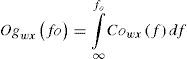

In the convergent case (Fig. 5a), the ogive function increases during the integration from high frequencies to low frequencies until a certain value is reached and remains on a more or less constant plateau before a 30-min integration time. If this condition is fullfilled, the 30-min covariance is a reliable estimate for the turbulent flux, because it is possible to assume that the whole turbulent spectrum is covered within that interval and there are only negligible flux contributions from longer wavelengths (case 1). But it can also occur that the ogive function shows an extreme value and decreases again afterwards (case 2, Fig. 5b), or that the ogive function does not show a plateau but increases throughout (case 3). Ogive functions corresponding to cases 2 or 3 indicate that a 30-min flux estimate is possibly inadequate. Foken et al. (2006) define thresholds for ogive characteristic behaviors in order to prescribe if an ogive belongs to case 1, 2 or 3.
From the ogive analysis performed for latent and sensible heat fluxes over the whole experimental period, the 30-min averaging interval appears to be sufficient to cover all relevant flux contributions with approximately 80% included in case 1, while only 20% belong to cases 2 and 3.
Finnigan et al. (2003) propose a site-specific extension of the averaging time up to several hours to close the energy balance. Figure 6 shows energy balance closures with reference to energy flux aggregations at different temporal scales.

The slope tends to increase if a large averaging time is considered, but if an aggregation period of 6h is examined, the linear regression (0.76) is quite similar to that calculated with half-hourly data (0.75). Instead, with an aggregation time period equal to 24 h, the slope has a large improvement (0.83). This is probably due to the effect of storage terms, which can be considered negligible at daily scale as shown in Foken (2008b).
3.4Effect of scale differences in flux measurementsThe energy balance closure can also be seen as a scale problem, because each flux is representative of an area (Fig. 7). In fact, the net radiometer source area is the field of view of the instrument at nadir related to the sensor height, and it doesn’t change with time. In Fig. 7a the net radiometer source area described by Schmid’s (1997) equation using the radiometer con Figuration on the tower for this experimental campaign, is shown. The radiometer is located on an arm (b) of about 2.5m long, attached to the tower at a height of about 4.5m (zr). Its orientation is from north to south in order to receive the whole solar radiation during the daily hours. Its source area has a circular shape with a maximum radius of about 4 m, and the major representativeness of the short and long wave measurement, which are coming from the surface, are in correspondence to the projection of the radiometer on the ground (red zones).
 Radiometer source area. (b) Footprint source area for eddy covariance instruments. (l) Arm length, (zr) radiometer height. The EC station comprises the eddy covariance instruments (gas analyzer and sonic anemometer). (zm) Hight of the eddy covariance instrument.")
The flux footprint of turbulent fluxes varies in space and time depending mainly on wind speed and direction, surface roughness, stability conditions of the atmosphere and measurement heights (Hsieh et al., 2000). According to Hsieh et al. (2000), the footprint represents a weight function (for unit of length) of different contribution that is coming from the surface area at a certain distance away from the instruments (anemometer and gas analyzer [EC station]). This function changes in space and time, and is different for each 30-min measurement. In Figure 7b, the footprint source area of the EC station considering the whole experimental data from May to September is shown. Bi-dimensional footprints are computed using Hsieh et al. (2000) and Detto et al. (2006) models for the longitudinal and lateral spreads, respectively. The mathematical approach to match Hsieh et al. (2000) and Detto et al. (2006) models is not described in this work but it is widely discussed in the recent article of van de Boer et al. (2013). The footprint area obtained for each half-hourly data has been oriented with respect to wind directions, and the footprint shape represented in Figure 7b has been obtained performing this procedure on the whole experimental data set. In general, the major representativeness of latent and sensible heat flux measurements is confined in an area of about 450 m2 on the right of the tower (west direction). This is probably due to the limited magnitude of wind intensities in the Po Valley, which do not exceed 10 ms-1 (Masseroni et al., 2014a, b).
The effect of flux spatial scales on the energy balance closure is evaluated considering the peak location of the footprint function inside the field. As shown in Figure 8, the peak data have been subdivided into four percentile groups (each with 25% of the data), so that turbulent fluxes of latent and sensible heat connected to each peak are used to compute the energy balance closure.
 of footprint functions, peak locations (xpeak).")
The energy balance closure tends to increase when the peak location is up to 22m away from the eddy covariance station. The maximum value of the linear regression slope is 0.88 in correspondence with the 75th percentile, i.e. with the footprint peak far from the tower, which varies between 10 and 22 meters. However, when the peak exceeds 22m the slope tends to decrease, probably because the representative source area of eddy covariance measurements exceeds the field dimensions. Instead, when the peak location is near the station the heterogeneity of the island surface and the influence of the devices could alter the turbulent flux measurements. The systematic error defined by intercept increases linearly with the percentile groups up to 9.7 Wm-2.
Ground heat flux is usually very small with respect to the other energy fluxes, ranging from 5 to 10% of the net radiation. However, the estimate of this flux has the highest uncertainty and can reach an error of up to 50% (Foken, 2008a). Moreover, it is measured with an instrument that has the smallest source area, which can be two orders of magnitude lower than the latent and sensible heat fluxes footprints, therefore it can vary greatly in the field due to different soil characteristics or soil moisture conditions, as shown in Kustas et al. (2000), who found that when measuring G with 20 different instruments in a small site, the mean differences in soil heat flux were about 40 Wm-2, but in some occasions they could deviate as much as 100 Wm-2. Research on the variation of heat soil flux across the fields and its influences on energy balance closure is an important issue which has been studied by many scientists. In the current state, G is assumed to be uniform on the field and its strong variability across the field is neglected in the first approximation.
3.5Effect of turbulent mixingThe effect of turbulent mixing is evaluated with respect to friction velocity (u*). Friction velocity typically changes with atmospheric stability and time of day, as explained by Wilson et al. (2002). Changes in the energy balance closure could also be the direct result of changes in friction velocity. In accordance with Wilson et al. (2002), a simple method to isolate the effects of friction velocity on energy balance improvement is shown. Data are separated into four 25-percentile groups, each group containing data where friction velocity is included between two consecutive friction velocity percentile values. The slope of linear regression R2 and intercept are also evaluated during daytime and nighttime, as shown in Figure 9. As explained in Figure 9a, during daytime the slope increases from 0.73 to 0.85 and the intercept varies from -1 to 2 Wm-2. Only when the friction velocity is included between 0.28 and 0.83 ms-1, the intercept collapses to a value of about 0.7 Wm-2. During nighttime (Fig. 9b) the energy balance closure is drastically worsen with a mean slope of about 0.06. The intercept is quite close to 0 Wm-2 while R2 considerably varies among the percentile groups. This is probably due to low wind velocities which, during nighttime, prevent the very turbulent mixed conditions of the atmosphere from increasing the advection transport of scalar fluxes and form worsening the eddy covariance measurements.
 Daytime, (b) nighttime.")
Figure 10 shows the friction velocity influence on energy balance closure, globally evaluated for the whole experimental data set. The slope constantly increases up to 0.82 when data are included in a friction velocity range between 0.24 and 0.83 ms-1. The systematic errors defined by intercept values tend to decrease and, in correspondence with a closure of 0.82, the intercept value is about 4.3 Wm-2. Literature results (Wilson et al., 2002; Barr et al., 2006) are also confirmed from the analysis performed at Livraga station, given that the closure of the energy budget tends to increase with the increase of friction velocity. In fact, when friction velocity is low, the turbulence is softened and the fluxes are usually underestimated. The problem related to the use of friction velocity as an indicator of good measured data is linked to a u* threshold definition. In Alavi et al. (2006) a value of 0.1 ms-1 is considered, while Oliphant et al. (2004) use 0.3 ms-1 and Barr et al. (2006) use 0.35 ms-1, showing that the choice of this limit on u* seems to be site dependent.
3.6Effect of vegetation
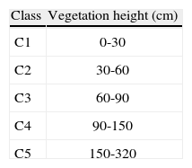
Many experimental results of energy balance problems related to low and tall vegetation are available in literature (Panin et al., 1998; Aubinet et al., 2000; Wilson et al., 2002). Here, the influence of vegetation height and heterogeneity on energy balance closure is studied subdividing the experimental data set into five classes from C1 to C5. Each class contains data with different vegetation heights (Table I) in function of canopy growth.
For each class, the energy balance closure is calculated and the results are shown in Figure 11a. The slope tends to decrease to 0.76 with the increase of vegetation height for a canopy height of 150 to 320cm. The maximum slope value is about 0.98 in correspondence with the C1 class when the surface heterogeneity is particularly accentuated. Intercept changes its positive sign in correspondence with the C5 class, where the intercept value is about -3.4 Wm-2. To better understand how these results are possible, the storage terms should be taken into account. In Figure 11b, the slopes of the linear regression are compared to the percentage storage weights defined in Eq. (7). Storage weight is the ratio between the averaged storage fluxes for each class and the sum of these averages on the whole class subdivisions.
where S is the storage term for the x flux (soil heat ground, photosynthesis or canopy storages), N is the number of data for each class and j is a class indicator that represents C1 when equal to 1, C2 when equal to 2, and so on.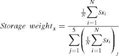
 Energy balance closure for five classes of vegetation height. (b) Slope and storage weight terms in function of vegetation height classes.")
As shown in Figure 11b, the slope trend is opposite to the canopy and the weight terms of photosynthesis storage. In fact, when canopy is tall the weights of Sc and Sp are particularly relevant, reaching a value of about 35% in correspondence with the C5 class. Instead, the weight term of soil heat ground storage drastically decreases when vegetation is tall, moving from 25 to 5% when the class changes from C4 to C5. The presence of vegetation covering the field plays a fundamental role in the energy balance closure. Particularly, the Sp and Sc storage terms increase their influence on energy balance closure during the canopy growth, and the energy unbalance is accentuated if they are not considered. When vegetation is decreased, Sp and Sc effects can be neglected while Sg becomes relevant, reaching the weight value of about 30% (C1 class).
3.7Effect of seasonalityThe daily patterns of the 30-min averages of Rn, LE, H and G in May, June, July and August are plotted in Figure 12 to clearly describe the partition of energy balance components during different seasons. The maximum peak of net radiation is quite constant from May to August, oscillating between 500 and 600 Wm-2. Latent and sensible heat have a strong variability trough the months, showing a quite similar trend from May to June, while in July and August latent heat is about three times greater than sensible heat. The soil heat flux accounts for a small proportion of the available energy, particularly when vegetation covers the field surface. In fact, during May it can also reach the maximum value of about 100 Wm-2 at 12:00, while in July and August soil heat flux is equal to a few tens of watt per square meter.
 May, (b) June, (c) July, (d) August.")
The partitioning of net radiation into sensible heat and latent heat fluxes is strongly influenced by change in vegetation characteristics. Specifically, when vegetation is tall, the dominant component of the energy budget is represented by latent heat, with a peak in July of about 450 Wm-2. Sensible heat is the main energy component when vegetation is absented; it tends to decrease during the canopy growth but, as shown in August, when vegetation is fully developed, it returns to similar values as those shown in May. A special phenomenon called “oasis effect” can be noted in July, when latent heat is the component that takes the largest portion of Rn and sensible heat is very small. In the case of optimum conditions for evaporation (i.e. high soil moisture and very turbulent conditions [Foken, 2008a]), the evaporation process is greater than sensible heat flux. In such cases, sensible heat changes its sign one to three hours before sunset and sometimes in the early afternoon, and a temperature gradient inversion along with a downward sensible heat transfer takes place in the atmosphere.
The energy balance closure for each month is shown in Figure 13. The slope of the linear regression is particularly influenced by the canopy growth. When the field is completely covered by vegetation and it can be considered as a homogenous surface, energy balance closure decreases up to 0.77 with an intercept value of about -1.4 Wm-2. This is probably due to the effect of the canopy and photosynthetic storage terms, which become important when vegetation is tall and the surface is homogenously covered by plants. When each flux of the energy balance over the whole experimental period is analyzed (Fig. 12), it is possible to realize that over a field covered by dense vegetation, latent heat is the main dominant component of the energy budget (with respect to sensible heat and soil heat ground) and the lack of the energy balance closure corresponds to an underestimation of the canopy evapotranspiration fluxes. In water management practices this problem assumes a dominant role in irrigation procedures, given that a correct estimation of evapotranspiration fluxes corresponds to an efficacious and sustainable management of the water resource.
3.8Random errors
The reliability of turbulent fluxes can be obtained only if the theoretical assumption of the eddy covariance technique (described in Moncrieff et al. [1996]) is followed. Non steady-state conditions, random noise of the signal, inadequate length of the sampling interval, size variation of the flux footprint and surface heterogeneity, single point measurement of the turbulence and inadequate sensor response, could cause random uncertainty in fluxes measurements. Random errors have been mainly studied by Hollinger and Richardson (2005), who compared flux measurements obtained by two identical micrometeorological stations located in the same place with the same flux footprint, or by Richardson et al. (2006), who compared a pair of measurements performed on two successive days from the same tower under equivalent environmental conditions. Using the Lenschow et al. (1994) method to detect random uncertainty in sensible and latent heat fluxes, it is possible to realize that errors in estimated means, variances and covariances diminish when the size of the data set is increased (as long as the data set is not enlarged in such a way that, for example, seasonal trends become important), and the random uncertainty magnitude proportionally increases with the growth of sensible and latent heat flux intensities (Fig. 14).
 and latent (b) heat fluxes magnitudes.")
Some authors as Bernardes and Dias (2010) include error bars when reporting measured values of turbulent fluxes. Though it is not a common micrometeorological practice, Figure 15 shows mean daily turbulent flux intensities together with their ranges of confidence, in order to explain how random errors affect latent and sensible heat fluxes. The maximum uncertainty is associated with daytime when maximum latent and sensible heat magnitudes are shown. During daytime, the maximum range of confidence is about 40 Wm-2 for sensible heat and 80 Wm-2 for latent heat, while during the nighttime it tends to zero.
 sensible and (b) latent heat fluxes.")
Generally, some random error sources could be solved by trying to apply rigorously practical rules described in many literature works, which have been written from the beginning of the eddy covariance technique (Schmid, 1997; Foken, 2008a). However, the energy balance closure is affected by these errors, which can not be completely eliminated. Filtering methods based on the spatial decomposition of turbulent fluxes (Salesky et al., 2012) try to quantify rigorously random errors, with the objective of including —in the common practice of the authors— an estimate of the random errors magnitude when micrometeorological measurements are shown.
4ConclusionsThe Livraga 2012 measurements are an excellent data set for evaluating the surface energy balance problems. All findings about flux error sources cannot completely explain the problem of unclosed surface energy balance. It was found that crucial attention to calibration, maintenance and software correction of data is essential to obtain half-hourly reliable fluxes. Despite this effort, the data set contains an unbalance of about 25%, which has been studied taking into account different turbulent flux problems.
Storage terms, which play a fundamental role in the improvement of the energy balance closure, are about 10% of the daily available radiation energy. Photosynthesis and canopy storage terms are prevalent in the field when vegetation covers the soil surface and canopy is fully developed. Ground heat storage is greater than the other storage terms, and it can reach up to 50% of the soil heat flux. Canopy growth and seasonality effects are strongly connected with storage terms. When vegetation is decreased the energy balance closure is almost equal to 1 because the only term that exists is the ground heat storage, with a percentage weight of about 30%. From class C1 to class C5 the energy balance closure decreases if the vegetation storage terms (canopy and photosynthesis) are not considered. Similarly, the energy balance closure decreases from May to August in accordance with the increasing of the vegetation storage terms. The energy balance flux partitioning highlights how available energy (net radiation) is subdivided into latent, sensible and soil heat fluxes, detecting the flux that could contribute most to the unbalance problem. During the experimental campaign, the results show that latent heat is the main component of the energy budget and, during some months, it is grater than 40% of the available energy.
Atmospheric turbulence characteristics play a fundamental role in reliable estimations of flux. In some cases, half-hourly averaged periods are not sufficiently large for taking into account the long-wave terms of turbulent flux measurements. Studying the ogive functions, the results show that about 20% of the data are partially corrected because their aggregation time covers only a portion of turbulent eddies, which stay in the surface layer (Garratt, 1993). Some authors, like Lenschow et al. (1994), suggest that the averaged aggregation time of the eddy covariance flux measurements should be changed in function of the atmospheric turbulence characteristics, but this method drastically increases the complexity of common practice measurements. The state of turbulent mixing is an important aspect against the advection phenomenon. One of the theoretical assumptions of the eddy covariance technique is that advection terms can be neglected. Friction velocity is used for providing a threshold that discerns the existing probability of advection transport. The energy balance closure in developed turbulent mixing conditions is greater than in cases with low turbulence, and the closure is about 0.8 if friction velocity is confined to 0.24-0.83 ms-1.
In the past, researches on energy balance closure problems were mainly directed to measuring errors, and only a few results underline the scale hypothesis. The results shown in this work underline the complexity of the source area footprint definition for each flux of the energy budget. Atmospheric stability conditions, measurement height, surface roughness and wind velocity are some common parameters that govern the footprint models. In the Po Valley, weak wind velocities and strong convective forces during the summer months cause the footprint movement to peak in direction of the tower, so that the major representativeness of the source area is certainly confined within the field. Site-specific experiments should be made to understand how the representative source area for the eddy covariance measurements change in function of atmospheric, physical and geometrical characteristics of the field. It should be a subject of further research to recalculate eddy covariance experimental results using a new experimental plan and a specialized measuring setup calibrated for the scale problem. LES modeling studies could be used to support these researches.
Despite the fact that this overview cannot be a final work, this paper shows important results about the energy balance closure problem. Moreover, it is one of the few researches on maize fields in the Po Valley presented in literature, increasing the knowledge on the energy balance problems at international scale.
This work was funded in the framework of the ACQWA EU/FP7 project (grant number 212250) “Assessing climate impacts on the quantity and quality of Water”, the framework of the ACCA project funded by Regione Lombardia “Misura e modellazione matematica dei flussi di ACqua e CArbonio negli agro-ecosistemi a mais” and PREGI (Previsione meteo idrologica per la gestione irrigua) founded by Regione Lombardia.