


Este trabajo presenta un estudio de la respuesta de la variabilidad simulada de la temperatura global a para-metrizaciones estocásticas aditivas y multiplicativas de flujos de calor, junto con una descripción de la variabilidad de largo plazo en términos de procesos autorregresivos simples. Para simular la temperatura global de la Tierra se utilizó un modelo climático de balance de energía promediado globalmente, acoplado a un modelo oceánico termodinámico. Se encontró que procesos autorregresivos simples explican la variabilidad de la temperatura en el caso de parametrizaciones aditivas; sin embargo, en el caso de parametrizaciones multiplicativas, la descripción de la variabilidad de la temperatura involucraría procesos autorregresivos de orden superior, lo cual sugiere la presencia de mecanismos complejos de retroefecto originados por el forzamiento multiplicativo. Asimismo, se encontró que las parametrizaciones multiplicativas produjeron una estructura compleja que emula de manera cercana procesos climáticos observados. Finalmente, se propone un nuevo enfoque para describir la estabilidad de un sistema estocástico general unidimensional en estado estacionario, a través de su función potencial. A partir de una expresión analítica de la función potencial se profundizó en la descripción de un sistema estocástico.
This work presents a study of the response of the simulated global temperature variability to additive and multiplicative stochastic parameterizations of heat fluxes, along with a description of the long-term variability in terms of simple autoregressive processes. The Earth's global temperature was simulated using a globally averaged energy balance climate model coupled to a thermodynamic ocean model. It was found that simple autoregressive processes explain the temperature variability in the case of additive parameterizations; whereas in the case of multiplicative parameterizations, the description of the temperature variability would involve higher order autoregressive processes, suggesting the presence of complex feedback mechanisms originated by the multiplicative forcing. Also, it was found that multiplicative parameterizations produced a rich structure that emulates closely observed climate processes. Finally, a new approach to describe the stability in the steady state of a general one-dimensional stochastic system, through its potential function, was proposed. From an analytical expression of the potential function, further insight into the description of a stochastic system was provided.
Estimating the effects that unresolved processes in the discretized domain (also called sub-grid scale processes) have on the variables of large scales (those that are resolved by the grid) is a central issue in climate modeling. Recently, the use of random processes for modelling events at these sub-grid scales has become a successful alternative to address the problem of unresolved scales (Benzi et al., 1981, 1982, 1983; Monahan et al., 2008; Williams, 2005; Penland and Ewald, 2008; Wilks, 2008). Nevertheless, the use of short-term random variations to mimic the behavior of processes of sub-grid scale significantly affects the dynamics of the climate system in the long term. The so-called dynamical-stochastic climate models are useful tools to try to explain the features and behavior of a climate model forced with random noise (von Storch and Zwiers, 1999).
Within the hierarchy of climate models of the atmosphere and ocean there are simple climate models (North et al., 1981; McGuffie and Henderson-Sellers, 2005; IPCC, 1997). The main application of these simple models is to advance in the understanding of the underlying dynamics of the climate system from a zero-order perspective. Specifically, various studies suggest that climate variability can be seen, to first order, as a simple auto-regressive process of order one or two (Hasselmann, 1976; von Storch and Zwiers, 1999; Mudelsee, 2010). It is therefore of interest to use a simple climate model driven by stochastic forcing to estimate the effect of random variability on some key factors of the climate system.
The first goal of this paper is to study the effects of stochastic parameterizations of heat fluxes on the variability of the global temperature, considering additive and multiplicative noise. The Earth's global temperature was simulated using a globally averaged energy balance climate model (EBCM) coupled to a thermodynamic ocean model, driven by stochastic forcing (stochastic EBCM). The differences between additive and multiplicative stochastic forcing were investigated and the long-term variability was described in terms of simple autoregressive models. From this study, an increased understanding of the description of the climate variability in the context of stochastic systems was obtained.
Additionally, studying a stochastic system through its potential function is important because it allows learning about its stability and behavior in the steady state. A number of studies describe a one-dimensional stochastic system driven by additive noise through its potential function (Nicolis and Nicolis, 1981; Wilks, 2008). However, the description of a one-dimensional stochastic system driven by multiplicative noise has not been sufficiently studied. So, the second goal of this paper is to provide further insight into the description of a general one-dimensional stochastic system through the concept of potential function, which will allow a simplified description of an inherently complex system.
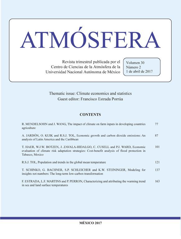
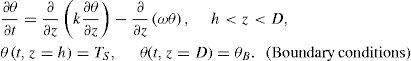
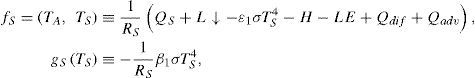
2Deterministic climate modelThe box-advection-diffusion model developed by Harvey and Schneider (1985) was used. This model represents a globally averaged energy balance climate model coupled to a one-dimensional, globally averaged ocean model. The ocean model consists of an isothermal mixed layer coupled to an advective-diffusive deep ocean (Fig. 1). The equations governing the evolution of the atmospheric temperature, TA (t), the oceanic mixed layer temperature, TS (t), and the deep ocean temperature, θ(t, z), where t represents time and z represents the depth of the ocean, are:


.")
The globally averaged box-advection-diffusion model. The straight arrows in the deep ocean represents advection and the wavy arrows represent diffusion. Also illustrated is a thermohaline circulation. Image taken from Harvey and Schneider (1985).
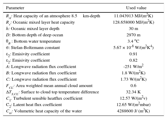
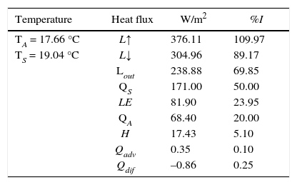
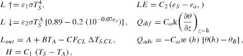
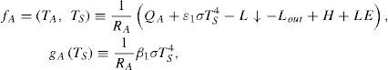
In the governing equations QA (68.4 W/m2) is shortwave radiation absorbed by the atmosphere, QS (171.0 W/m2) is shortwave radiation absorbed by the oceanic mixed layer, L↑ is upward emitted surface longwave radiation, L↓ is downward emitted atmospheric longwave radiation, Lout is longwave radiation emitted to space at the top of the atmosphere, H is turbulent sensible heat flux, LE is latent heat flux, Qdif is diffusive heat flux and Qadv is advective heat flux. These heat fluxes are given by the following conventional deterministic parameterizations, whose physical parameters and used values are listed in Table I.
Physical parameters and used values.
| Parameter | Used value |
|---|---|
| RA: Heat capacity of an atmosphere 8.5km-depth | 11.043913 MJ/(m2K) |
| Rs: Oceanic mixed layer heat capacity | 128.658000 MJ/(m2K) |
| h: Oceanic mixed layer depth | 30 m |
| D: Bottom depth of deep ocean | 2970 m |
| θB : Bottom water temperature | 3.4 oC |
| σ: Stefan-Boltzmann constant | 5.67 × 10⁻⁸ W/(m2K4) |
| ε2: Emisivity coefficient | 0.91 |
| ε2: Emisivity coefficient | 0.82 |
| A: Longwave radiation flux coefficient | -251 W/m2 |
| B: Longwave radiation flux coefficient | 1.8 W/(m2K) |
| C: Longwave radiation flux coefficient | 1.73 W/(m2K) |
| FCL: Area weighted mean annual cloud amount | 0.6 |
| ΔTS,CL: Surface to cloud top temperature difference | 32.34 K |
| C1. Turbulent sensible heatflux coefficient | 12.57 W/(m2v) |
| C2: Latent heat flux coefficient | 12.65 W/(m2mbar) |
| Cω: Volumetric heat capacity of the water | 4288600 J/ (m3K) |
with the surface saturation vapor pressure (ea [mbar]) and atmosphere vapor pressure (ea [mbar]) calculated using a fixed relative humidity r = 0.71,

According to the results of Kunze et al. (2006) and Wunsch and Ferrari (2004), in a global average it is appropriate to use constant values of the diffusion coefficient, k, and of the speed of advection, ω. For k a constant value (1.0 ×10⁻⁵ m2/s) was used, whereas for the advection speed a steady profile which decreases in magnitude with depth z was used, ω(z) = 0.045 cm/day [–1 + 0.08 tanh (0.001 m–1 • z – 0.03)].
To integrate numerically the advection-diffusion equation ([Eq. 3]) a modified version proposed by Grima and Newman (2004) was used. The first derivative (both temporal and spatial) was approximated as a simple forward finite difference, whereas a central differences scheme was used for the higher order derivatives. A time step of one day and a vertical grid with 297 points with spacing of10 m were used. The model was started from initial conditions TA (t = 0) = TS (t = 0) = θ (t = 0, z) = θB, and integrated until an equilibrium state was reached after 3000 years (Table II). This state was then used as the initial condition for the stochastic formulation of the climate model.
Mean values of atmospheric and oceanic mixed layer temperatures and of heat fluxes as obtained in the steady state. A value of 342 W/m2 for the global average insolation I at the top of the atmosphere was used.
| Temperature | Heat flux | W/m2 | %I |
|---|---|---|---|
| TA = 17.66 °C | L↑ | 376.11 | 109.97 |
| TS = 19.04 °C | L↓ | 304.96 | 89.17 |
| Lout | 238.88 | 69.85 | |
| QS | 171.00 | 50.00 | |
| LE | 81.90 | 23.95 | |
| QA | 68.40 | 20.00 | |
| H | 17.43 | 5.10 | |
| Qadv | 0.35 | 0.10 | |
| Qdif | –0.86 | 0.25 |
One of the goals of this work is to study the response of the global temperature variability to perturbations represented by both additive and multiplicative noise terms. According to Deser et al. (2010), the energy fluxes from the ocean to the atmosphere strongly depend on a single oceanic quantity, the sea surface temperature (SST), which then represents a key factor regulating climate and its variability. Additionally, the heat fluxes from the ocean to atmosphere depend on several atmospheric parameters like air temperature, wind speed, humidity and cloudiness.
Therefore, the following regimes of stochastic forcing were considered: (1) random variations of the net flow of energy into the ocean (represented as additive noise), and (2) random variations in the upward emitted surface longwave radiation (represented as multiplicative noise). The reason for considering only a physical process was to separate the effect of each one of them on the evolution of the ocean-atmosphere system. The derivation of stochastic differential equations for each of the proposed cases is presented below, where the relevant stochastic processes were introduced using white noise, i.e., in form of increments of a Wiener process (Higham, 2001).
3.1Additive noise: random forcing in the oceanThis stochastic forcing can be seen as a radiative forcing (W/m2), i.e., it can be understood as fast random atmospheric heat flux fluctuations that are disturbing the energy flow from the atmosphere into the oceanic mixed layer,
where βS is a parameter which regulates the intensity of the fast random radiative forcing and ξ(t) is a Gaussian white noise process. In terms of increments of a Wiener process (dW = ξ[t] dt), the Ito version of the stochastic differential equation for TS is expressed as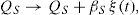

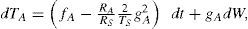
The random term in (4) (βSdW/RS) does not depend on the state of the system, so the random term represents additive noise.
3.2Multiplicative noise: stochastic parameterization of L↑The proposed stochastic parameterization ofthe heat flux L↑ considers that the emissivity coefficient ε1 is not constant in time, but fluctuates randomly following a Gaussian distribution around its deterministic value. The emissivity coefficient ε1 was replaced according to
where β1 regulates the intensity of the fluctuations of the new coefficient of emissivity. This results in a state-dependent (multiplicative noise) parameterization of Li, i.e., the values of L↑ are dependent on TS, L↑ = [ε1 + β1ξ (t)] σTS4 So, the resulting equations for TA and TS represent Stratonovich stochastic differential equations,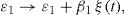


In order to apply the standard methods of Ito calculus, these equations were ex-pressed in terms of the Ito formulation (Jacobs, 2010),
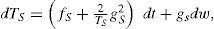
where the following functions have been defined,
For each case, the Ito stochastic differential equations ([Eqs. 4], [7] and [8]) were solved numerically and the corresponding sample paths were obtained. A time step of one day for both the discretized Brownian path and for the Euler-Maruyama numerical integration was used (Higham, 2001). The simulation time was 2000 years.
4ResultsIn this section the evolution of the atmosphere-ocean system was investigated. The short-term and longterm variability for additive and multiplicative forcing were analyzed and the null hypothesis for climate variability proposed by Hasselmann (1976) was tested. This hypothesis states that to a first order of approximation, the long-term variability can be explained by a simple autoregressive process.
4.1Additive noise: random forcing in the oceanFigure 2 shows a scatter plot of the standardized anomalies series of TS and TA for the daily and annual time scales. This figure hints at a positive correlation in the daily scale, with a Pearson's correlation coefficient of 0.9906, which gets stronger in annual scales, with a Pearson's correlation coefficient of0.9998. Due to the interconnection of the ocean-atmosphere system and to the fact that climatic processes are predominantly determined by the ocean, it is possible to define a causality relation between the two temperatures: the atmosphere's evolution is strongly determined by the ocean's state, i.e., “the atmosphere follows the ocean”.

To see the behavior of the ocean-atmosphere system, Figure 3 shows the time series of the standardized anomalies of TA and TS and their corresponding autocorrelation function (ACF), for the daily and annual time scales. In Figure 3a it is observed that in short time scales the ocean temperature has more variability than the atmospheric temperature. This is just a consequence of the mathematical fact that the stochastic forcing was added to the flux of incident energy into the ocean, causing short-term random variations in TS (one day in the numerical model).

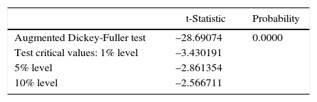
The ACFs of TA and TS decay very slowly in the daily time scale (Fig. 3b), with significant correlations at 4380 lags (12 years). Despite the slow decay rate of the ACFs, both of the daily time series are stationary, which was proved by the Augmented Dickey-Fuller test (see Appendix A). It is clear that due to the larger heat capacity of the ocean with respect to the atmosphere, the persistence of the ocean should be higher than the persistence of the atmosphere. However, due to the structure of the random forcing (no state-dependent noise), the persistence of both atmosphere and ocean is exactly the same (Fig. 3b, c, d), which is unrealistic.
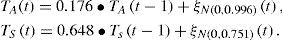
To test the null hypothesis for climate variability, simple autoregressive models were fitted to the standardized anomalies of TA and TS (see Appendix A).
Daily data:

Annual data:
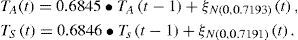
Figure 4 shows smoothened Fourier spectra of the standardized anomalies of TA and TS for the daily and annual time scales, which were calculated averaging eight replicated spectra without overlap (Wilks, 2011) and compared with the theoretical spectra of the corresponding fitted autoregressive models. The light-gray line stands for the atmosphere sample spectrum and the dark-gray line for the ocean sample spectrum. The solid and dashed lines indicate the theoretical spectrum of the estimated autoregressive model and the 95% confidence level for the ocean, respectively. The dashed-dotted and dotted lines indicate the theoretical spectrum of the estimated autoregressive model and the 95% confidence level for the atmosphere, respectively.

The strong coupling between ocean and atmosphere is demonstrated by the high grade of similarity between their spectra. Both spectra show a higher spectral density at low frequencies and lower density at high frequencies (red noise or positive persistence processes). The theoretical spectra of the fitted autoregressive models were used to prove the statistical significance of the higher amplitudes of the corresponding sample spectra. The analysis revealed that with 95% confidence level, the variability of the ocean and atmosphere temperatures could be described in terms of purely random processes. For the case of additive forcing the obtained response is entirely consistent with the Hasselmann's hypothesis of climate variability, although some results of this case are unrealistic.
4.2Multiplicative noise: stochastic parameterization of L↑The proposed stochastic parameterization of L↑ yields some interesting results, the first of which concerns the anticorrelation between ocean and atmosphere temperatures (Figs. 5 and 6a). The Pearson's correlation coefficient has a value of –0.8426 for the daily time scale and a value of –0.3965 for the annual time scale.


In the deterministic steady state both fA and fS are zero (i.e., the heat fluxes in the ocean-atmosphere system are balanced) and then they do not affect the evolution of global temperatures. So, the anticorrelation is caused by the random terms gA and gs. An explanation of this behavior emerges by considering a discretized version of Eqs. (7) and (8), in which the deterministic terms are null (fA = fS = 0),
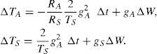
Combining these equations, it is obtained
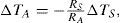
which explains the negative correlation between TS and TA and the relative amplitude of their variations, given by the quotient RS/RA (≈ 11.65). In fact, stochastic parameterizations of any heat flux will produce a similar anticorrelation pattern, a loss of energy by the atmosphere (decreases in TA) will be balanced by a gain of energy by the ocean (increases in TS), and vice versa. The anticorrelation will not be perfect due to the differences in the heat capacity of the atmosphere and ocean.
Anticorrelated multidecadal variations between SST and subsurface ocean temperature has been reported for the tropical North Atlantic (Zhang, 2007). Further insight into this anticorrelation might be obtained in the frame of simplified stochastic models. It is speculated that a similar mechanism might be present between the surface and the subsurface ocean temperatures.
As it is expected, the persistence of the ocean is higher than the persistence ofthe atmosphere (Fig. 6b). The ocean integrates the random short-term atmospheric variations producing an amplified response on the long-term variability due to its large heat capacity (Dommenget and Latif, 2002). For the annual time scales and due to the strong anticorrelation between atmosphere and ocean, the integration of the shortterm variations produced a positive high long-term persistence for the ocean temperatures and a negative low long-term persistence for the atmosphere temperatures (Figs. 6c, d). The observed negative feedback in the atmosphere in the annual time scales causes the atmosphere temperature to oscillate rapidly around its mean value.
To investigate the null hypothesis of climate persistence, simple autoregressive models were fitted to the standardized anomalies of TA and TS (see Appendix A).
Daily data:

Annual data:
The estimations indicate that for the daily time scale the fitted models for the atmosphere and ocean are very similar, which suggests that for short periods the same autoregressive model can be used to describe the short-term variability of the atmosphere and the ocean. However, the atmosphere has a greater standard deviation of white noise than the ocean, which leads to a greater variability in the short term with respect to the ocean. For the annual time scale, the atmosphere has a low negative persistence, while the ocean has a positive persistence. These features are better represented by the Fourier spectra of both standardized anomalies (Fig. 7). Nomenclature is the same as for the additive noise case.
At long periods (> 4 years) there is a net energy flux towards the ocean such that the spectral density of TS continues to increase with decreasing frequency, being unbounded at these frequencies (< 0.25/year). Its spectral density is higher than that of the fitted autoregressive model at long periods. So, the TS long-term variability cannot be described using a simple autoregressive process and the null hypothesis of climate variability must be rejected (Fig. 7a). However, for the annual average the TS long-term variability can be very well described by a simple autoregressive model (Fig. 7b).

The unboundedness of the TS spectrum for the daily data, characteristic not observed in the case of additive (no state-dependent) noise, was entirely caused by the inclusion of multiplicative (state-dependent) noise. A comparable spectrum behavior was reported by Dommenget and Latif (2002), who compared spectra of observed monthly mean SST with simulations carried out with fully dynamical ocean models. They found an increased variance ofthe SST on seasonal and decadal time scales relative to the fitted AR(1) process. This continuous reddening of the spectrum at long time scales could be originated by many different dynamical processes interacting and producing variance at these time scales (Vallis, 2010). In the present work, nevertheless, the only reason for such behavior was the inclusion of multiplicative noise.
Concerning the TA long-term variability (Fig. 7a, b), it is observed that the spectral density of TA for both time scales is lower than the spectral density of the fitted autoregressive model at long periods. So, the TA long-term variability cannot be adequately described using a simple autoregressive process and the null hypothesis of climate variability must be rejected. Also, a negative feedback (increasing spectral density with increasing frequency) in the atmosphere is observed. Negative climate feedbacks have been documented in literature. Kärner (2002) carried out a statistical analysis for satellite-based global daily tropospheric (6-8 km depth) and stratospheric (15-19 km depth) temperature anomalies, from 1979 to 2001. He found antipersistency in the daily increments of the tropospheric temperature for scales longer than two months, pointing at a negative feedback governing the tropospheric variability.
The determining factor for long-term persistence in an AR(1) process is the persistence term (Wilks, 2011; Brooks, 2008). The equations that describe the evolution of atmospheric and oceanic temperatures contain state-dependent noise, which introduces a reformulation of the underlying deterministic behavior that governs them ([Eqs. 7] and [8]). Thus, more complex feedbacks between the two components are incorporated, which do not correspond to a simple autoregressive process. The complexity of these feedback mechanisms can lead to more complex time series models or to non-linear models (Mudelsee, 2010). Further research is needed to address the complexity of these mechanisms.
5Potential function in the steady state of a stochastic systemThis section reviews the calculation of the potential function in the steady state of a system described by a one-dimensional general Ito stochastic differential equation,

where x(t) is the stochastic process, t is time, f(x,t) is the deterministic term, g(x,t) is the random term and dW are the increments of a Wiener process. Knowledge ofthe potential function in the steady state shall provide useful information about the behavior of x(t) when t → ∞, independently of the initial conditions taken on Eq. (10).
Based on the probability density function (PDF) in the steady state, the potential function V(x) is defined. It is assumed that in the steady state it is possible to establish a correspondence between the PDF and the potential function V(x). The aim of this section is to show a general procedure to calculate an analytical expression for the potential function associated to a general one-dimensional Ito stochastic differential equation.
The traditional approach (of classical physics) applied to the calculus of the potential function considers it in terms of a generalized force. This approach has been used in the analysis of one-dimensional stochastic differential equations forced with additive noise (g = constant). Nicolis and Nicolis (1981) and Wilks (2008) found the following expression to calculate the potential function Vˆx,
which coincides with the deterministic case g = 0, usual in classical physics. However, in the case of one-dimensional stochastic differential equations forced with multiplicative noise (g = g[x]), an analytical expression for the calculation of the potential function is not available.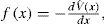
Unlike the traditional approach ([Eq. 11]), the definition of the potential function here is in terms of the steady PDF of the stochastic process, and not in terms of a generalized force. From the steady PDF P(x), the extrema of P(x) were found, which ought to be equal to the extrema of V(x). Then, in order to ensure the correspondence between P(x) and V(x), it had to be ensured that the maxima of P(x) corresponded with the minima of V(x) and vice versa, which was proven by applying the criterion of the second-order derivative. This ensures that V(x) characterizes the PDF globally, not just at the extrema.1
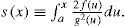
In order to illustrate this new approach, the stochastic system in Eq. (10) with reflecting boundaries conditions within the domain x ∈a,b was considered. The expression for its steady probability density, obtained form solving the Fokker-Planck equation, is (Jacobs, 2010)
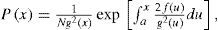
where N is a normalization constant that satisfies P(x) = 1. The first-order derivative of P(x) is
with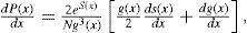
Thus, the potential function V(x) can be defined through the relation
which guarantees that P(x) and V(x) have the same extrema xc. In order to ensure that V(x) characterizes the PDF globally, the maxima of P(x) have to coincide with the minima of V(x), and vice versa. The second-order derivative of P(x) evaluated at the extrema xc is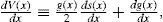
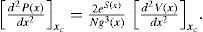
Considering g x<0 ∀x, the expression (16) becomes
and the condition that the maxima of P(x) coincide with the minima of V(x), and vice versa, is fulfilled. If g x>0 ∀x it is sufficient to define the potential function with a global minus sign to ensure that Eq. (15) remains valid. On the other hand, if g(x) shows alternations of sign within the considered domain, the total domain can be divided into subintervals where the function g(x) has a unique sign. Then the described procedure can be applied to each subinterval performing the adequate modifications.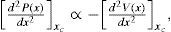
By substituting Eq. (14) into Eq. (15) and using Leibniz's rule, the final expression for calculating the potential function in the steady state is
where it was assumed that f is a C2 class function and g is a C1 class function.
In the case of additive noise (g[x] = constant and not null) Eq. (18) is reduced to the expression found by Nicolis and Nicolis (1981) and by Wilks (2008) (Eq. [11]). Despite the fact that the general procedure to calculate the potential function described here was developed considering reflecting boundaries, it is suitable for application to other types of boundary conditions.
The result expressed by the relation in Eq. (18) evidences that the potential function associated with a stochastic process depends strongly on the random term g(x). The behavior of the system can be modified considerably regarding its deterministic behavior (g = 0) or its behavior with additive noise forcing (g = constant), by the presence of state-dependent stochastic forcing (g = g[x]). So, the approach shown here for the calculation of the potential function represents a useful tool for the analysis of a stochastic system of the kind expressed in Eq. (10) in the steady state.
5.1Application to the stochastic climate modelThe approach shown above is not applicable to coupled systems. For that purpose further investigation is required. It is not possible to apply this procedure to the stochastic climate model developed in this work. Nevertheless, if some strong considerations are taken, it is possible to calculate the potential functions which determine the behavior of TA and TS in the steady state.
Even though Eqs. (4) (for additive noise) and (7) and (8) (for multiplicative noise) involve the three temperatures TA, TS and θ, these equations can be considered univariate after the substitution of the independent variables for their value in the deterministic equilibrium (Table II). This is adequate because the structure and intensity of the introduced stochastic forcings (section 3) are such that temperatures TA and TS oscillate exclusively around their values in the deterministic equilibrium. That is, the calculations can be made in a univariate framework.
Figures 8 and 9 show the steady PDF (Eq. [12]) and the potential function (Eq. 18]) of ocean (TS) and atmosphere (TA) temperatures for the proposed cases of stochastic forcing. In both cases it was found that within the considered domain the potential function has only one minimum, which represents the only stable state and coincides with the maximum of the corresponding PDF. The maxima of the PDFs and the minima of the potential functions coincide with the corresponding values of the temperatures in the deterministic equilibrium (Table II). In the case of multiplicative forcing (Fig. 9), the potential function for TS is flatter than the potential function for TA (Fig. 8), so the PDF for TS is broader than the PDF for TA. Finally, for both cases of stochastic forcing, the potential functions, the PDFs and the deviations of temperatures around their deterministic value are symmetrical.
 and steady probability density function (solid line) for the ocean temperature. Random forcing in the ocean.")
 and steady probability density function (solid line) for ocean (left panel) and atmosphere temperatures (right panel). Stochastic parameterization of L↑.")
This paper shows that simple climate models are useful for understanding the fundamental characteristics of the climate system, but they do not provide a detailed description thereof. By representing some unresolved processes in the climate system by noise terms in the differential equations that govern them, the Hasselmann's hypothesis of climate variability was investigated for the cases of additive and multiplicative stochastic forcing. When the system is forced with additive noise, its response can be adequately described, to a first order of approximation, by simple autoregressive processes; whereas when the system is forced with multiplicative noise, a description of its response would involve higher order time series models or even non-linear models. In contrast with additive forcing, multiplicative forcing produced a rich structure that closely emulates some observed climate processes both in the atmosphere and in the ocean. The conducted analysis with this simplified climate model suggests that a more accurate description of the climate variability can be obtained in the framework of stochastic models with multiplicative forcing.
Another result of this work was the derivation of an analytical expression to calculate the potential function of a general one-dimensional stochastic differential equation, which gives a clear idea of the behavior of the variable of interest in the steady state, before solving the respective stochastic differential equation. By providing a view of the stability of a system, this approach can be used in the study of noise-induced transitions between different stable states or in the study of stochastic resonance (Gammaitoni et al., 1998), both of which play an important role in climate research (Williams, 2005; Monahan et al., 2008).
To estimate the autoregressive models the methodology developed by Box and Jenkins (1970) was used. This methodology is based on the use of graphic tools, like the autocorrelation function (ACF) and the partial autocorrelation function (PACF) to identify the appropriate model to be fitted. The estimation method used was the least squares method. All of the calculations were carried out using the econometric package EViews 9.0.
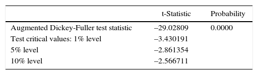
First of all, the non-stationarity of the daily temperature series was tested. The stationarity of a series was taken in the context of weak stationarity: constant mean, constant variance and constant autocovariances for each given lag. The null hypothesis (the series contain a unit root) was tested using the Augmented Dickey-Fuller test. The results are shown in Tables A.I and A.II. It is observed that, for both TA and TS, the values of the test statistics are more negative than the corresponding critical values, so the null hypotheses of a unit root were rejected.
The PACFs and the tables of analysis of variance (ANOVA) for the daily and annual time scales and for each temperature are shown below.
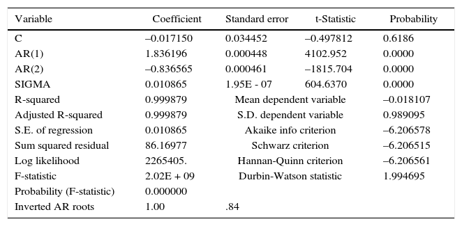
Model estimation for the daily standardized anomalies of TA. Random forcing in the ocean.
| Variable | Coefficient | Standard error | t-Statistic | Probability |
|---|---|---|---|---|
| C | –0.017150 | 0.034452 | –0.497812 | 0.6186 |
| AR(1) | 1.836196 | 0.000448 | 4102.952 | 0.0000 |
| AR(2) | –0.836565 | 0.000461 | –1815.704 | 0.0000 |
| SIGMA | 0.010865 | 1.95E - 07 | 604.6370 | 0.0000 |
| R-squared | 0.999879 | Mean dependent variable | –0.018107 | |
| Adjusted R-squared | 0.999879 | S.D. dependent variable | 0.989095 | |
| S.E. of regression | 0.010865 | Akaike info criterion | –6.206578 | |
| Sum squared residual | 86.16977 | Schwarz criterion | –6.206515 | |
| Log likelihood | 2265405. | Hannan-Quinn criterion | –6.206561 | |
| F-statistic | 2.02E + 09 | Durbin-Watson statistic | 1.994695 | |
| Probability (F-statistic) | 0.000000 | |||
| Inverted AR roots | 1.00 | .84 | ||
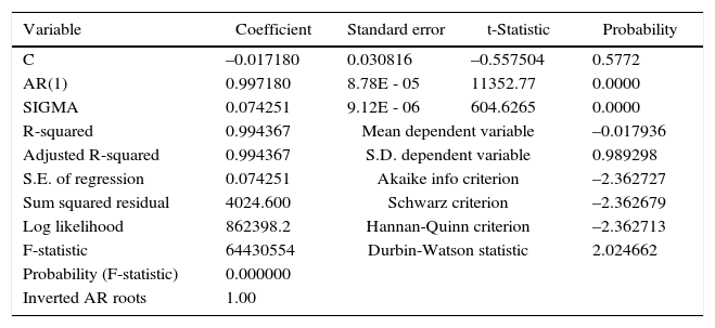
Model estimation for the daily standardized anomalies of TS. Random forcing in the ocean.
| Variable | Coefficient | Standard error | t-Statistic | Probability |
|---|---|---|---|---|
| C | –0.017180 | 0.030816 | –0.557504 | 0.5772 |
| AR(1) | 0.997180 | 8.78E - 05 | 11352.77 | 0.0000 |
| SIGMA | 0.074251 | 9.12E - 06 | 604.6265 | 0.0000 |
| R-squared | 0.994367 | Mean dependent variable | –0.017936 | |
| Adjusted R-squared | 0.994367 | S.D. dependent variable | 0.989298 | |
| S.E. of regression | 0.074251 | Akaike info criterion | –2.362727 | |
| Sum squared residual | 4024.600 | Schwarz criterion | –2.362679 | |
| Log likelihood | 862398.2 | Hannan-Quinn criterion | –2.362713 | |
| F-statistic | 64430554 | Durbin-Watson statistic | 2.024662 | |
| Probability (F-statistic) | 0.000000 | |||
| Inverted AR roots | 1.00 | |||
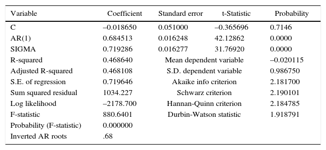
Model estimation for the annual standardized anomalies of TA. Random forcing in the ocean.
| Variable | Coefficient | Standard error | t-Statistic | Probability |
|---|---|---|---|---|
| C | –0.018650 | 0.051000 | –0.365696 | 0.7146 |
| AR(1) | 0.684513 | 0.016248 | 42.12862 | 0.0000 |
| SIGMA | 0.719286 | 0.016277 | 31.76920 | 0.0000 |
| R-squared | 0.468640 | Mean dependent variable | –0.020115 | |
| Adjusted R-squared | 0.468108 | S.D. dependent variable | 0.986750 | |
| S.E. of regression | 0.719646 | Akaike info criterion | 2.181700 | |
| Sum squared residual | 1034.227 | Schwarz criterion | 2.190101 | |
| Log likelihood | –2178.700 | Hannan-Quinn criterion | 2.184785 | |
| F-statistic | 880.6401 | Durbin-Watson statistic | 1.918791 | |
| Probability (F-statistic) | 0.000000 | |||
| Inverted AR roots | .68 | |||
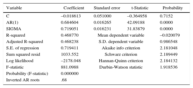
Model estimation for the annual standardized anomalies of TS. Random forcing in the ocean.
| Variable | Coefficient | Standard error | t-Statistic | Probability |
|---|---|---|---|---|
| C | –0.018613 | 0.051000 | –0.364958 | 0.7152 |
| AR(1) | 0.684604 | 0.016265 | 42.09188 | 0.0000 |
| SIGMA | 0.719051 | 0.016231 | 31.83879 | 0.0000 |
| R-squared | 0.468770 | Mean dependent variable | –0.020079 | |
| Adjusted R-squared | 0.468238 | S.D. dependent variable | 0.986548 | |
| S.E. of regression | 0.719411 | Akaike info criterion | 2.181048 | |
| Sum squared resid | 1033.552 | Schwarz criterion | 2.189449 | |
| Log likelihood | –2178.048 | Hannan-Quinn criterion | 2.184132 | |
| F-statistic | 881.0988 | Durbin-Watson statistic | 1.918536 | |
| Probability (F-statistic) | 0.000000 | |||
| Inverted AR roots | .68 | |||
PACFs and ANOVAs for the daily and annual time scales and for each temperature are shown below.
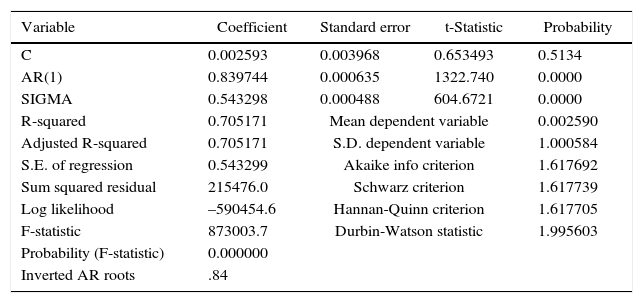
Model estimation for the daily standardized anomalies of TA. Stochastic parameterization of L↑.
| Variable | Coefficient | Standard error | t-Statistic | Probability |
|---|---|---|---|---|
| C | 0.002593 | 0.003968 | 0.653493 | 0.5134 |
| AR(1) | 0.839744 | 0.000635 | 1322.740 | 0.0000 |
| SIGMA | 0.543298 | 0.000488 | 604.6721 | 0.0000 |
| R-squared | 0.705171 | Mean dependent variable | 0.002590 | |
| Adjusted R-squared | 0.705171 | S.D. dependent variable | 1.000584 | |
| S.E. of regression | 0.543299 | Akaike info criterion | 1.617692 | |
| Sum squared residual | 215476.0 | Schwarz criterion | 1.617739 | |
| Log likelihood | –590454.6 | Hannan-Quinn criterion | 1.617705 | |
| F-statistic | 873003.7 | Durbin-Watson statistic | 1.995603 | |
| Probability (F-statistic) | 0.000000 | |||
| Inverted AR roots | .84 | |||
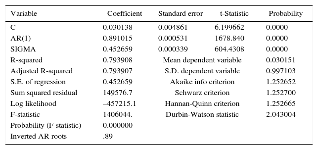
Model estimation for the daily standardized anomalies of TS. Stochastic parameterization of L↑.
| Variable | Coefficient | Standard error | t-Statistic | Probability |
|---|---|---|---|---|
| C | 0.030138 | 0.004861 | 6.199662 | 0.0000 |
| AR(1) | 0.891015 | 0.000531 | 1678.840 | 0.0000 |
| SIGMA | 0.452659 | 0.000339 | 604.4308 | 0.0000 |
| R-squared | 0.793908 | Mean dependent variable | 0.030151 | |
| Adjusted R-squared | 0.793907 | S.D. dependent variable | 0.997103 | |
| S.E. of regression | 0.452659 | Akaike info criterion | 1.252652 | |
| Sum squared residual | 149576.7 | Schwarz criterion | 1.252700 | |
| Log likelihood | –457215.1 | Hannan-Quinn criterion | 1.252665 | |
| F-statistic | 1406044. | Durbin-Watson statistic | 2.043004 | |
| Probability (F-statistic) | 0.000000 | |||
| Inverted AR roots | .89 | |||
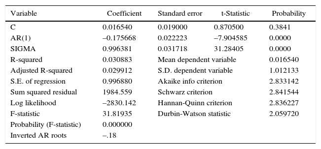
Model estimation for the annual standardized anomalies of TA Stochastic parameterization of L↑.
| Variable | Coefficient | Standard error | t-Statistic | Probability |
|---|---|---|---|---|
| C | 0.016540 | 0.019000 | 0.870500 | 0.3841 |
| AR(1) | –0.175668 | 0.022223 | –7.904585 | 0.0000 |
| SIGMA | 0.996381 | 0.031718 | 31.28405 | 0.0000 |
| R-squared | 0.030883 | Mean dependent variable | 0.016540 | |
| Adjusted R-squared | 0.029912 | S.D. dependent variable | 1.012133 | |
| S.E. of regression | 0.996880 | Akaike info criterion | 2.833142 | |
| Sum squared residual | 1984.559 | Schwarz criterion | 2.841544 | |
| Log likelihood | –2830.142 | Hannan-Quinn criterion | 2.836227 | |
| F-statistic | 31.81935 | Durbin-Watson statistic | 2.059720 | |
| Probability (F-statistic) | 0.000000 | |||
| Inverted AR roots | –.18 | |||
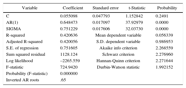
Model estimation for the annual standardized anomalies of TS. Stochastic parameterization of L↑.
| Variable | Coefficient | Standard error | t-Statistic | Probability |
|---|---|---|---|---|
| C | 0.055098 | 0.047793 | 1.152842 | 0.2491 |
| AR(1) | 0.648473 | 0.017097 | 37.92979 | 0.0000 |
| SIGMA | 0.751229 | 0.017606 | 32.03730 | 0.0000 |
| R-squared | 0.420636 | Mean dependent variable | 0.056339 | |
| Adjusted R-squared | 0.420056 | S.D. dependent variable | 0.986953 | |
| S.E. of regression | 0.751605 | Akaike info criterion | 2.268559 | |
| Sum squared residual | 1128.124 | Schwarz criterion | 2.276960 | |
| Log likelihood | –2265.559 | Hannan-Quinn criterion | 2.271644 | |
| F-statistic | 724.9420 | Durbin-Watson statistic | 1.992152 | |
| Probability (F-statistic) | 0.000000 | |||
| Inverted AR roots | .65 | |||