


En los últimos años se ha generado en México, así como alrededor del mundo, un gran interés de la comunidad científica por tener un mayor conocimiento acerca del comportamiento de los eventos climáticos extremos, debido a su creciente número e intensidad. El objetivo de esta investigación fue realizar un análisis de eventos climáticos extremos de temperatura utilizando para ello índices extremos de clima. Se efectuó un estudio de caso para el municipio de Apizaco, Tlaxcala, México, con series de datos de temperaturas máxima y mínima diarias para el periodo 1952-2003. Se calcularon seis índices relacionados con temperatura máxima y mínima: días de heladas, días de verano, días cálidos, días fríos, noches cálidas y noches frías. Los resultados de todos ellos se evaluaron de forma anual, y sólo cuatro se analizaron por temporadas. Se les ajustó una tendencia con un modelo de regresión lineal de mínimos cuadrados, para determinar su comportamiento. Los resultados de los índices mostraron que los eventos extremos relacionados con temperatura máxima tuvieron más cambios, los días de verano se incrementaron y los días fríos disminuyeron. Además, hubo un incremento en los días de heladas, es decir, se presentó una mayor cantidad de días con temperaturas mínimas por debajo de 0° C. En general, los resultados indicaron que se están presentando temperaturas más extremas, más cálidas pero también más frías. La detección de estas tendencias en los eventos extremos se puede considerar como un primer paso en cualquier estudio de atribución de los cambios observados (v. gr., cambios en el uso del suelo, cambio climático regional, etc.). Este aspecto de atribución no se abordará en el presente trabajo.
In recent years in Mexico and around the world, the scientific community has shown great interest in acquiring knowledge regarding the behavior of extreme climate events due to their increasing number and intensity. The objective of this research was to analyze variations in extreme temperature events using extreme climate indices. We conducted a case study for the municipality of Apizaco, Tlaxcala, Mexico, using data sets of the daily maximum and minimum temperatures for the period from 1952 to 2003. Six indices related to maximum and minimum temperatures were calculated: frost days, summer days, warm days, cool days, warm nights and cool nights. All of the index results were evaluated annually and only four of the indices were analyzed according to the seasons. A trend based on a linear least squares regression model was fit to the indices to determine their behavior. The index results showed that extreme events related to maximum temperatures corresponded to greater changes and an increased number of summer days and decreased cool days. Additionally, there was an increase of frost days, associated with a greater number of days with minimum temperatures below 0 °C. In general, the results indicated that warmer and colder extreme temperatures are occurring. The detection of those trends in the extreme events can be seen as a first step in any study of the attribution of those observed changes (e.g., land use change, regional climate change, etc.). This attribution aspect will not be discussed in the present study.
Two aspects of climate that may be modified by current climate changes are extreme temperature and precipitation events, and we must prepare for outcomes of these events that may affect the population, infrastructure, systems and sectors, for example. Extreme events can cause short- or long-term side effects. Therefore, there is an obvious need within the scientific community, as well as public and private sectors, to investigate extreme climate events and their possible effects in response to current and future climate change.
According to the Intergovernmental Panel on Climate Change “...an extreme weather event is an event that is rare at a particular place and time of year. Definitions of rare vary, but an extreme weather event would normally be as or rarer than the 10th or 90th percentile of the observed probability density function. When a pattern of extreme weather persists for some time, such as a season, it may be classed as an extreme climate event, especially if it yields an average or total that is itself extreme (e.g., drought or heavy rainfall over a season)” (IPCC, 2007). Climate change resulting from human influences has led to changes in the frequency and intensity of extreme events. To support these conclusions, the IPCC (Solomon et al., 2007) emphasizes that “...specialized statistical methods based on quantitative analysis have been developed for the detection and attribution of climate change”.
In this paper, methods to analyze the observed changes in extreme events are applied, but no attempt is made to attribute these changes to anthropogenic causes of climate change. Consequently, research has emerged that is focused on developing methods for evaluating these events to estimate the possible effects of observed climate change (Rosenzweig et al., 2007). One method that has been used for the analysis of extreme events, which arose from the need to determine whether extreme was changing, was the characterization of extreme events within a region using indices. Currently, the Expert Team on Climate Change Detection Monitoring and Indices (ETCCDMI), sponsored by the Commission for Climatology (CC1) of the World Meteorological Organization and the Climate Variability and Predictability project (CLIVAR, http://www.clivar.org/), defines 27 base indices (Zhang and Yang, 2004; Peterson, 2005) that are related to temperature and precipitation, which have been employed in several investigations related to extreme events (Frich et al., 2002; Klein Tank and Können, 2003; Rusticucci and Barrucand, 2004; Aguilar et al., 2005; Kostopoulou and Jones, 2005; Vincent et al., 2005; Alexander et al., 2006; Hernández, 2006; Sillmann and Roeckner, 2008).
The objective of this paper is to present a methodology based on indicators for the analysis of temperature extreme events in a case study site, the municipality of Apizaco in the state of Tlaxcala, Mexico and to detect whether these types of events are changing.
2Case study and dataTo illustrate the methodology used in the extreme events analysis, we conducted a case study for the municipality of Apizaco, Tlaxcala, Mexico. Apizaco is located in the Central Mexican Plateau at 2380 m above sea level, with geographic coordinates between 19° 29’-19° 22’ N and 98° 03’-98° 11’W, in the central area of Tlaxcala state and with an exent of 43.46km2 (Fig. 1). According to geostatistics information of the Instituto Nacional de Estadística y Geografía (INEGI, National Institute of Statistics and Geography), the Apizaco municipality represents 1.14% of the total state territory (3991.14km2). Rain-fed agriculture is the principal economic activity of Apizaco and is practiced in 98% of the municipality; this activity is threatened by extreme events, such as frost, drought and torrential rains. The climate of Apizaco is considered to be temperate sub-humid with rainfall during the period of May through mid-October. The wind direction is generally from north to south. The recorded average annual maximum and minimum temperatures were 22.5 and 4.7 °C, respectively. Average annual rainfall recorded during the period 1961-1990 in the municipality was 812.1mm and annual average evapotranspiration for the same period was 4.9mm/day (htxtp://smn.cna.gob.mx/).

One of the large-scale phenomena that influence the climate of Apizaco is the El Niño/Southern Oscillation (ENSO). During strong El Niño events, summer rain is usually below normal and the frost-free period is reduced (Gay et al., 2004), increasing the risk of unexpected frosts. In contrast, during strong La Niña events above normal summer precipitation is expected (Conde et al., 2000).
Due to the rare occurrence of extreme events, it is necessary to investigate such occurrences using daily and long-term observation records to determine significant changes in these events. It is also necessary that the data sets are homogeneous and reliable, i.e., that there are no instrumental, human, or environmental errors that may alter the results. The data used in this study correspond to the weather station 029002 (19° 25’ N-98° 09’ W) that was located outside the city of Apizaco during the period 1952-2003, so the results presented here cannot be attributed to an urban heat island effect.
The series of daily maximum temperature (Tmax) and minimum temperature (Tmin) can be obtained by the Computerized Climate database (CLICOM, CLima COMputarizado) (http://data.eol.ucar.edu/codiac/dss/id=82.175). These datasets were used and validated in previous studies (i.e., Conde et al., 2006), which analyzed also critical values during extreme conditions (such as strong ENSO events).
Regardless of those previous analyses, the Tmax and Tmin databases were subjected to a quality control to identify possible errors (i. e., Tmin > Tmax) that could affect the results of this study.
3MethodologyThe methodology used in the evaluation of extreme events consisted of three main parts that were intended to address different aspects of extreme temperature events (López, 2009).
3.1Characterization of the local climatologyKnowledge of the behavior of the local climate is required because extreme events can vary from region to region. In addition, a seasonal classification can be performed to identify the occurrence of extreme temperatures and to further clearly delineate hot and cold temperatures without altering the subsequent results. In this case, the observed climate was described using Tmax and Tmin over a baseline period, which included 30 years of observed meteorological data, as suggested by the World Meteorological Organization (WMO). For a description of the data behavior during the baseline period (1961 to 1990), it was necessary to apply descriptive statistics tools, which include measurements of the location, dispersion and symmetry of the data (Wilks, 1995). In addition, graphical methods were used to visually assess the data and detect any unusual observations, such as transcription errors or so-called outliers (i. e., atypical values outside the expected range).
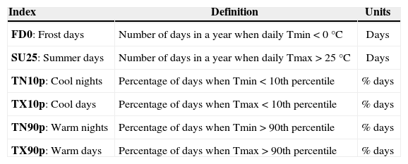
3.2Calculation of indices of extreme climate eventsThe indices used to characterize extreme events were those defined by the ETCCDMI (Zhang and Yang, 2004; Peterson, 2005). From the set of indicators, six related to temperature were chosen, that characterized the variations in day and night temperature according to Tmax and Tmin, respectively (Table I).
Climatic indices of the maximum and minimum temperatures as provided by the Expert Team on Climate Change Indices and Detection.
| Index | Definition | Units |
|---|---|---|
| FD0: Frost days | Number of days in a year when daily Tmin < 0 °C | Days |
| SU25: Summer days | Number of days in a year when daily Tmax > 25 °C | Days |
| TN10p: Cool nights | Percentage of days when Tmin < 10th percentile | % days |
| TX10p: Cool days | Percentage of days when Tmax < 10th percentile | % days |
| TN90p: Warm nights | Percentage of days when Tmin > 90th percentile | % days |
| TX90p: Warm days | Percentage of days when Tmax > 90th percentile | % days |
Source: Zhang and Yang, 2004.
The frost days (FD) and summer days (SU) indices are determined by thresholds and are defined as the number of days for which the assessed values are greater than or less than a predetermined value. The determination of the threshold depends on the studied region because each threshold is regional. The cool nights (TN10p), cool days (TX10p), warm nights (TN90p) and warm days (TX10p) indices are quantified as percentiles, i.e., they represent the extremes of a distribution and indicate the coldest and warmest deciles, which are used for assessing the changes in these extremes (Alexander et al., 2006).
In general, most of the indices can be applied to any area of the world; however, certain indices may not be significant when the climatic differences between regions and their interpretation are considered (Tebaldi et al., 2006).
The indices were calculated with the help of the computer program RClimDex, which is free software (http://cccma.seos.uvic.ca/ETCCDI/software.shtml), running on the R platform (http://www.r-project.org/). RClimDex performs the index calculations using daily data and provides monthly and yearly data. It includes a data quality control, which was useful to construct the database used in this study.
3.3Setting the trendsOne approach to understanding the behavior of extreme events and therefore whether the events are changing, is to set a trend for the series of indices resulting from previous analysis. In this case, the trends were fitted using a least squares linear regression model:

where y is the dependent variable, xj the independent variable, C a constant coefficient, aj the regression parameter and e the residual (constant with zero variance). To validate the model, specification tests were performed, including statistical tests on the coefficients and model parameters. With this model structural changes in the series can be identified (using the Quandt-Andrews test) and observations considered to be outliers can be normalized. The structural changes and outliers were introduced into the model as dummy variables (Brooks, 2008). This form of adjustment has been employed in works related to trend analyses in Mexico (SUMA, 2011).
Several of the outliers can be associated to critical years in the region of Tlaxcala, including the municipality of Apizaco. That is the case of the severe cold winters and very hot summers during strong El Niño events (such as 1982-1983 and 1997-1998 [Conde and Eakin, 2003; Conde et al., 2006]). Very low temperatures occurred during December 1989, when frost events affected several states in Mexico (such as Tlaxcala, Puebla, Hidalgo and Veracruz). These outliers were preserved in the analysis of the series, but did not determine their trend.
4ResultsWhen characterizing the temperature variability in Apizaco, the monthly maximum temperature (Fig. 2a) was shown to be 20.4 °C in January and subsequently increased from February to May; a temperature maximum of 25.1 °C was recorded in May. For the month of June, there was an abrupt decrease of 2.0 °C, which coincided with the onset of the summer rains. This finding indicates that water evaporation was favored when there was an increased amount of incident radiation, thereby forming a large extent of cloudiness, lowering the incident radiation and decreasing the warming of the surface. This situation will correspond to low Tmax values. Beginning in June, there was a steady trend of decreasing Tmax values, although a “small” increase in the median Tmax for the month of August was observed (however this trend was not clear), which could have been related to a heat wave or drought season (Conde et al., 1999; Magaña et al, 1999). In the following months, a decreasing trend in Tmax, down to 20.4 °C in December, was observed, which coincided with decreasing temperatures in autumn and winter.
: (a) maximum temperature; (b) minimum temperature")
For the monthly minimum temperatures (Fig. 2b), although the incident radiation—and therefore the emission of infrared radiation—increased in the winter months, this radiation was not trapped by the atmosphere due to insufficient atmospheric water vapor (i.e., these are cold and dry months). This produced an effect called “radiation frost” that must affect agricultural activities. In January, a value of 0.2 °C was recorded. After this month, Tmin increased until it reached a maximum value of 8.2 °C in the month of June, which was opposite to the Tmax trend, which began to decline at this point because the “cumulative” radiation on the surface began to escape in the form of longwave radiation (i.e., heat). In June, Tmin reached a maximum, thereby favoring evaporation and an increase in cloudiness. This situation, as mentioned above, blocks the incident radiation, thereby causing Tmax to decrease. At this point Tmin decreased; it appeared to be largely stable in July, August and September and decreased again during October through December.
It is possible to develop a seasonal classification based on the climatology description and the monthly Tmax and Tmin. In this case, three classifications were identified: the first classification groups the cold months of January, February and March (Temp1); the second includes the warm months from April to September (Temp2); and the third is composed of the cold months of October, November and December (Temp3). In this manner, it is possible to analyze the results of those indices that provide monthly results.
The trends were fitted using a linear regression model to a 5% significance level. For the annual data, the adjusted trends showed that those indices related to the maximum temperature, such as summer days (SU25: Tmax > 25 °C) had significant increases; i.e., there was a greater number of days in the year that exceeded 25 °C, which is related to more extreme daily Tmax values (Fig. 3a). The most outstanding events of SU25 occurred during 1998 (El Niño year, during January to April) with 118 days and also during 1982 (El Niño event, from May to December) with 99 days.
 Summer days (SU25: Tmax > 25 °C), (b) frost days (FD0: Tmin < 0 °C); in both cases we found a significant positive trend (with significance at the 5% level). In the graphs, the solid line is the series of data observed (“actual”) and the dotted line is the trend (“fitted”)")
In addition, the trend adjustment for the percentage of cool days (TX10p: Tmax < 10th percentile) indicated that there was a structural change in 1964, which meant that from this year onward, there was an increase in cool days; however, since this break, the trend showed a significant decrease. Meanwhile, the number of warm days (TX90p: Tmax > 90th percentile) increased, although the trend was not significant. The highest percentage of warm days occurred in 1998 (27.5%) and 1982 (21.2%), two years of strong El Niño events.
With respect to the indices related to the minimum temperatures, the frost days (FD0: Tmin < 0 °C) showed a significant positive trend with a structural change in 1977. This breaking point was negative, which means that after this point, there was a decrease in the mean of frost days; however, this number subsequently increased. In general, the increase in frost days indicated that there were more days with Tmin below 0 °C, which corresponded to the most extreme low temperatures (Fig. 3b). The indicators of cool nights (TN10p: Tmin < 10th percentile) and warm nights (TN90p: Tmin > 90th percentile) showed no changes in their trends. In those series of cool nights, the most notable event occurred during 1982, an El Niño year, with 28.3% of days below the 10th percentile.
Table II shows a summary of results of the indices that were calculated annually: the trend coefficient value, its significance at the 5% level (S if it is significant and NS non-significant) and structural changes (on average) observed for each index series.
Value trends, significance and structural changes in the annual trends of Apizaco, Tlaxcala
| Index | Trend coefficient | Probability | Significance probability < 0.05 | Structural changes |
|---|---|---|---|---|
| FD0: Frost days* | 1.107103 | 0.0008 | S | 1977 |
| SU25: Summer days* | 0.574041 | 0.0055 | S | ---- |
| TN10p: Cool nights** | 0.073071 | 0.1725 | NS | ---- |
| TX10p: Cool days** | −0.257972 | 0.0000 | S | 1964 |
| TN90p: Warm nights** | 0.033992 | 0.5126 | NS | ---- |
| TX90p: Warm days** | 0.011689 | 0.7873 | NS | ---- |
The calculation of percentile trends provides monthly results; therefore, a seasonal analysis can be performed and additional detailed information can be obtained.
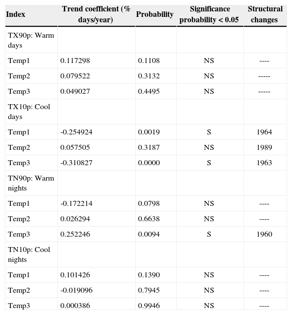
The trends for warm days (TX90p) in the three seasons were not significant; however, this index appeared to be increasing and if this trend continues, warmer Tmax values could occur. In Temp2, during an El Niño event in 1998, the maximum of warm days (47%) was recorded.
The indicator of cool days (TX10p) showed a significant negative trend in the cold months (Temp1 and Temp3), which may indicate that fewer maximum temperature values were less than the 10th percentile. i. e., these values were warmer. Structural changes were present in the three seasons: in Temp1 and Temp3, the breaks correspond to the years 1964 and 1963. respectively. Therefore, prior to these years, the mean of cool days was decreasing and then a subsequent increase likely occurred due to cooling in the region, followed by a further decrease (Fig. 4a, 4c).
 in the three seasons: (a) Temp1 (January to March); (b) Temp2 (April to September); and (c) Temp3 (October and November). Structural changes were observed in all cases. In Temp1 and Temp3 the trends were negative (with significance at the 5% level). The solid line represents the series of data observed (“actual”) and the dotted line represents the trend (“fitted”)")
Cool days (TX10p) in the three seasons: (a) Temp1 (January to March); (b) Temp2 (April to September); and (c) Temp3 (October and November). Structural changes were observed in all cases. In Temp1 and Temp3 the trends were negative (with significance at the 5% level). The solid line represents the series of data observed (“actual”) and the dotted line represents the trend (“fitted”)
For Temp2 (April-September), there was a structural change in 1989; i.e., from 1952 up until the break, the mean of cool days increased in the warm season and subsequently decreased after this break. Overall, significant decreases in the cool days index were observed in the seasons (Fig. 4b), and this was reflected in the annual trend.
In the case of the warm night’s percentage (TN90p), the annual results showed an increase that was non-significant. When the seasonal division was performed, TN90p increased significantly during the cold season, Temp3, which also presented a structural change in 1960. After that break, there was a decrease in the mean of the warm night’s index, which subsequently increased, thereby indicating that Tmin may have been warmer for this season (Fig. 5). The opposite trend occurred in Temp1, which corresponds to the colder months, although the decrease was not significant. Temp2 showed no clear trend.
 in Temp3, showing a trend of increase (its significance at the 5% level) and a structural change in 1960. The solid line represents the series of data observed (“actual”) and the dotted line represents the trend (“fitted”)")
For Temp1, the cool nights index (TN10p) showed an increasing behavior; however, this trend was non-significant. For Temp2 and Temp3, the trends were unchanged; in all three cases, no structural changes were observed.
Table III shows the results for the percentile indices divided into the three seasons based on local climatology: trend coefficient, the probability value and its significance at the 5% level (S is significant and NS non-significant), and the observed structural changes.
Trend coefficients, significance and structural changes for the percentile indices according to season in Apizaco, Tlaxcala.
| Index | Trend coefficient (% days/year) | Probability | Significance probability < 0.05 | Structural changes |
|---|---|---|---|---|
| TX90p: Warm days | ||||
| Temp1 | 0.117298 | 0.1108 | NS | ---- |
| Temp2 | 0.079522 | 0.3132 | NS | ----- |
| Temp3 | 0.049027 | 0.4495 | NS | ----- |
| TX10p: Cool days | ||||
| Temp1 | -0.254924 | 0.0019 | S | 1964 |
| Temp2 | 0.057505 | 0.3187 | NS | 1989 |
| Temp3 | -0.310827 | 0.0000 | S | 1963 |
| TN90p: Warm nights | ||||
| Temp1 | -0.172214 | 0.0798 | NS | ---- |
| Temp2 | 0.026294 | 0.6638 | NS | ---- |
| Temp3 | 0.252246 | 0.0094 | S | 1960 |
| TN10p: Cool nights | ||||
| Temp1 | 0.101426 | 0.1390 | NS | ---- |
| Temp2 | -0.019096 | 0.7945 | NS | ---- |
| Temp3 | 0.000386 | 0.9946 | NS | ---- |
Based on the results presented above, it can be concluded that the maximum temperature index clearly shows a significant increasing trend, which may imply the presence of extreme Tmax values. In contrast, Tmin showed no significant changes, although an extremely cold Tmin may occur, especially for the period from January to March.
5ConclusionsUsing the proposed methodology, it is possible to characterize extreme temperature events. This methodology can be applied in other regions of study to determine whether extreme events are changing, thus fulfilling one of the greatest present day challenges, mainly in Mexico, where detailed studies have not been performed. The results obtained from the analysis of extreme events can be tailored to meet the needs of specific sectors, such as agriculture and healthcare, to better inform decision-making processes.
Critical years can be detected during the analysis, such as those extremes associated with strong El Niño events. Nevertheless, in the study of the trends of extreme temperatures, those values are considered as outliers and incorporated as dummy values in the model used to establish the significance of the trends and the structural changes.
In the case of Apizaco, Tlaxcala, only specific indices of extreme Tmax and Tmin events showed significant trends. However, certain indices showed an increase in Tmax and a decrease in Tmin. The most consistent change, both annually and seasonally, was observed for the number of cool days, which are decreasing at the study site, thereby implying an increase in Tmax minimums. Therefore, the behavior of the indices indicates the occurrence of extreme maximum temperatures with greater changes and extreme minimum temperatures with fewer variations, although with a possible decreasing trend.
This methodology has been used as a tool to detect observed changes in regional temperature extremes. The obtained results can be used in future studies to attribute these changes to factors such as land use change or regional climate change. The observed changes described in this paper could be attributed to climate change only if those changes are “...(1) unlikely to be due entirely to natural internal climate variability; (2) consistent with estimated or modeled responses to the given combination of anthropogenic and natural forcing; and (3) not consistent with alternative, physically plausible explanations of recent climate change” (Rosenzweig et al., 2007).