


Las sequías ocurren cuando las lluvias disminuyen o cesan durante días, meses o años. En el último quinquenio se registraron varias sequías meteorológicas en Venezuela, las cuales impactaron negativamente los sectores hidroeléctrico y agrícola. En este trabajo se desarrolló y validó un modelo de alerta temprana para la ocurrencia de sequías meteorológicas en el país, con el objeto de proporcionar a las instituciones que administran los recursos hídricos una herramienta que permita mejorar la planificación de su uso. Para desarrollar el modelo se utilizaron las series pluviométricas de 632 estaciones. La identificación de los episodios secos se realizó a través del índice estandarizado de precipitación (SPI, por sus siglas en inglés). Se utilizó un análisis de componentes principales asociado a un sistema de información geográfica para delimitar subregiones homogéneas (SH) geográficamente continuas, según el SPI. En cada SH se seleccionó una estación representativa (estación de referencia, ER) y se aplicó un análisis de correlación desfasada entre las series SPI en las ER y series de anomalías de 10 índices de variables macroclimáticas (VM). Las cuatro VM desfasadas con mayor correlación lineal en cada ER se organizaron en tres niveles (-1, 0 y +1), usando los cuartiles Q2 y Q4 como valores de truncamiento. Las series SPI se expresan en cuatro rangos: no seca, moderadamente seca, severamente seca y extremadamente seca. Se determinó la probabilidad condicional de ocurrencia de los cuatro rangos de SPI en cada combinación en que pueden presentarse las cuatro VM desfasadas. Se validaron los modelos en cada ER con las series de SPI provenientes de 20 estaciones pluviométricas del Servicio de Meteorología de la Fuerza Aérea Venezolana. Los resultados indican que los modelos detectan la ocurrencia de eventos ES con un acierto que varía de 85.19 a 100%; el acierto es directamente proporcional a la longitud de los registros usados en el desarrollo del modelo. El método puede aplicarse en cualquier país que disponga de series pluviométricas largas, continuas y homogéneas.
Droughts occur when rainfalls diminish or cease for several days, months or years. In the last five years several meteorological droughts have occurred in Venezuela, impacting negatively water supply, hydro-power and agriculture sectors. In order to provide institutions with tools to manage the water resources, a probabilistic model has been developed and validated to predict in advance the occurrence of meteorological droughts in the country using monthly series of 632 rainfall stations. The standardized precipitation index (SPI) was used to identify dry events of each rainfall series. A principal component analysis associated to a geographic information system was used to define geographically continuous homogeneous sub-regions (HS) for the values of SPI. For each HS a representative station was selected (reference station, RS). A lagged correlation analysis was applied to the SPI series of the RS and the corresponding series of anomaly indices of 10 macroclimatic variables (MV). The four MV with higher correlation in each RS were organized into three levels (-1, 0 and +1), using the quartiles Q2 and Q4 as values of truncation. The SPI series are expressed in four ranges: non-dry, moderately dry, severely dry and extremely dry. The conditional probability of occurrence of the four ranges of SPI was determined in every combination that can occur in the four VM best correlated. The resulting model in each RS was validated using the SPI series from 20 meteorological stations operated by the Servicio de Meteorología de la Fuerza Aérea Venezolana (Meteorological Service of the Venezuelan Air Force) which were not used in the development of the models. Results indicate that models detected the occurrence of ES with an accuracy ranging from 85.19 to 100%; the success is directly proportional to the length of records used in the development of the model. This methodology could be applied in any country that has long, continuous and homogeneous rainfall series.
In the last decade the frequency of occurrence of extreme meteorological droughts in South America has increased. During 2005, the river flows of southwest Amazonia were strongly affected by drought (Marengo, 2009); in 2009, fires in Colombia destroyed 13 000 hectares of forest and farmland as a result of droughts; in late 2010, Uruguay and Argentina declared a national joint emergency responding to a drought that was spread in both nations. In the same period, Bolivia also suffered severe socioeconomic damages as a consequence of droughts, especially in the cattle industry sector. Extreme dry seasons occurred in Venezuela from 2001 to 2003 and in 2007, causing an alarming reduction of reserves in the dams that supply water systems in the country and forcing water companies to implement rigorous rationing plans in major cities. In 2010 the occurrence of a persistent drought caused a significant reduction in the contribution of flow to the Simón Bolívar hydroelectric power station, creating huge gaps in the supply of energy, due to the fact that this plant provides over 90% of hydropower and 65% of the total energy consumed in the country. This event prompted the Venezuelan state to enact a power-rationing program for almost a year.
Due to the geographical location of Venezuela (north of South America, between 1-12° N and 60-74° W) the spatial and temporal distribution of rainfall is influenced largely by alternating migration of the Inter-Tropical Convergence Zone (ITCZ), which is the main mechanism for generating rainfall in the area. The dry season occurs during the astronomical winter (November-March) as a consequence of an anticyclonic situation in height, which affects almost the entire country. There is an inversion in the middle of the troposphere, which inhibits the formation of cloud cores of major vertical development. During this season, localized convective rains of short duration and high intensity occur, as well as some tropical disturbances, such as residual cold fronts of subtropical origin that favor the occurrence of atypical rainfall in some areas, particularly the coastline area (Velásquez, 2000).
The spatial and temporal pattern of rainfall and the geographical location of major urban and industrial centers of the country, play an important role in the management of water resources because a great part of the population is concentrated in areas of lower water availability. In the south of the Orinoco River the use of water resources does not cause conflicts between different users because its availability is far larger than the demand; however, the vulnerability to droughts increases in the region of the coastline and coastal mountain range due to increased population density and the resulting industrial development, which causes a water deficit by increasing the magnitude of demand. The vulnerability is also due to the following factors related to the characteristics of climate: (1) about 95% of the country’s reservoirs are located in watersheds with arid or semi-arid weather; (2) larger units of agricultural production (livestock and cereal production) are concentrated in Venezuelan plains, where a system of rainfed production prevails; (3) most of the agribusiness sector uses cereals to produce food for massive consumption, so the domestic market for grain, meat products and sub-products is directly affected by the occurrence of drought that persists for several days or months in the primary production units; and (4) only 5.7% of Venezuela’s farmlands have operating irrigation systems (Ovalles et al, 2007).
Extreme rainfall events (droughts and torrential rains) in Venezuela are related to the occurrence of one of the stages of the El Niño-Southern Oscillation (ENSO) phenomenon, with persistent thermal anomalies in the surface of the North and South Atlantic Ocean and/or inversion in the direction and intensity of winds over the tropic. These synoptic conditions in the ocean-atmosphere subsystems and their interactions influence the spatial and temporal distribution of rainfall (Cárdenas et al, 2002; Mendoza and Puche, 2005; Paredes et al, 2007). Consequently, it appears that the analysis of the dependence between meteorological droughts and macroclimatic variables, expressed as standardized anomalies, could be a useful tool to predict the occurrence of such meteorological droughts in Venezuela (Martelo, 2004; Guevara and Paredes, 2007; Paredes and Guevara, 2008). A first approximation to this method was proposed by Paredes and Guevara (2010) with the aim to predict the occurrence of early meteorological droughts in some homogeneous sub-regions of Venezuelan’s plains (depending on the inter-annual severity of the dry season), with satisfactory results.
Despite the economic impacts that droughts have always caused, Venezuela does not have a formal early warning system for extreme weather phenomena. However, it should be said that the Servicio de Meteorología de la Aviación Militar Venezolana (SEMETAVIA, Weather Service of the Venezuelan Military Aviation), in conjunction with the Observatorio Nacional de Eventos Extraordinarios (ONE, National Observatory of Extraordinary Events) of the University of Zulia, has been using experimentally the climate predictability tool (CPT) developed by the International Research Institute for Climate and Society (IRI) to produce forecast maps of rainfalls at national, seasonal and quarterly scales. CPT uses three statistical methods: (1) canonical correlation analysis, (2) principal components regression, and (3) multiple linear regressions. The predictor variables are: sea surface temperature (SST) in the Niño3 region of the Pacific, North and South Atlantic, and Caribbean Sea, measured in the previous month of the quarter to be forecasted (CIIFEN, 2010). SEMETAVIA produces monthly a thematic map with regional iso-probability of precipitation for the quarter evaluated. The main limitations of the CPT are: (1) it does not consider predictors associated with the atmosphere subsystem, and (2) it uses a constant gap of three months between the predictors and rainfall in the reference stations of SEMETAVIA. Some constraints are considered, because certain variables associated with wind fields in the upper troposphere, such as the quasi-biennial oscillation at 50mb (QBO50), can modulate the severity of extreme rainfall events (Cárdenas et al, 2002); on the other hand, a highest degree of linear association between macroclimatic variables and precipitation can also occur at different lags, including a three months lag (Martelo, 2004).
To provide a tool to the Venezuelan water resources authority that aids to confront the droughts and reduce their impacts, a model was developed and validated to predict the early occurrence of such phenomenon based on the conditional probability of the standardized precipitation index (SPI) of McKee et al. (1993). This article describes the fundamentals of the model, the methodology used and the main results.
2Data and methodology2.1 Study areaThis study covers the entire surface of the Bolivarian Republic of Venezuela and uses four variables of Pacific Ocean El Niño sub-regions, two variables of the Atlantic Ocean (north and south) and one variable of the Caribbean Sea, as indicated in Figure 1.
2.2Research phases2.2.1Phase I. Regionalization of rainfall anomalies
1. A preliminary database (PDB) was developed with 632 weather stations in Venezuela that have rainfall records. The information concerning the PDB were longitude, latitude, serial, name, type, state where the stations are located, operating agency, and period (starting year-final year).
2. From the PDB, stations with rainfall series that met the following criteria were selected: (a) 20 or more years of continuous records (no missing data), and (b) homogeneous series of annual rainfall, as monitored by the statistical test of Easterling et al. (1996). The AnClim software (Štěpánek, 2005) was used for the analysis. The selected series were called sample series (SS). The use of the climatic standard proposed by the WMO (1990) and discussed by Guttman (1998) was discarded, because of the heterogeneity in the beginning and ending dates of the series and the high percentage of missing data (climatic normals 01/01/1961 to 31/12/2000). Due to their different lengths of records, SS were divided into two groups:
- (a)
SS of the northern side of the country, consisting of 234 stations located at the north of the Apure and Orinoco rivers, with a common record period from 1983 to 1993; and (b) SS of the southern side comprising the states of Delta Amacuro, Bolívar, Apure, and Amazonas with 23 stations and a common period from 1971 to 1991.
3. The SPI of McKee et al. (1993) was calculated for every station in both groups. The SPI series obtained as indicated are hereafter referred to as north SS and south SS.
4. The normality of the frequency distribution of north and south SS series was checked using the Shapiro-Wilk W test (de la Fuente, 2005) and the STATISTICA 7™ software. Only 247 stations passed the normality W test (p < 0.01). At this point, stations without a normal frequency distribution were discarded.
5. A principal component analysis (PCA) with Varimax rotation and Kaiser normalization (Pérez, 2004) was applied separately to both groups of stations (north and south SS) that passed the normality W test. The SPSS 10™ software was used with following results:
- (a)
For the north SS group, the sampling adequacy measure of Kaiser-Meyer-Olkin was 0.697 (KMO index); the Bartlett test of sphericity was significant (χ2 = 62268.174, p < 0.01); and 42 factors were retained with auto values greater than one, explaining 78.69% of the total variance. The reproduced correlation matrix has 154 non-redundant residues with absolute values greater than 0.05 (< 1%).
- (b)
For the south SS group, the sampling adequacy measure of Kaiser-Meyer-Olkin was 0.924 (KMO index); the Bartlett test of sphericity is significant (χ2 = 2939.16, p < 0.01); and four factors are retained with auto values greater than one, explaining 60.18% of the total variance. The reproduced correlation matrix has 81 non-redundant residues with absolute values greater than 0.05 (32%).
6. To classify the stations (north and south SS), the rotated component matrices generated as explained in the previous point were used, according to the belonging factor given by the PCA analysis (32 groups on the north and four on the south).
7. The stations and their corresponding factor were depicted on a geographic information system (GIS) developed using the software ArcMap™ 9.2; closed polygons were drawn around the stations having a common factor, and stations geographically located outside with continuous polygons were discarded. In this manner 31 polygons were generated, which are here referred as homogeneous sub-region (HS). The stations grouped in each HS were characterized by their spatial coverage, altitude above sea level, mean annual rainfall, and occurrence of the dry season identified by a rainfall coefficient (Carrillo, 1999).
8. A representative station was selected for each HS based on the following criteria: (1) the SS of the station has the largest record of observation; (2) the station’s altitude, mean annual rainfall and dry season have the highest percentage of occurrence. The selected station is called hereafter reference station (RS). A total of 29 RS were generated in this way, which represent from the statistical point of view all of the stations included in one HS.
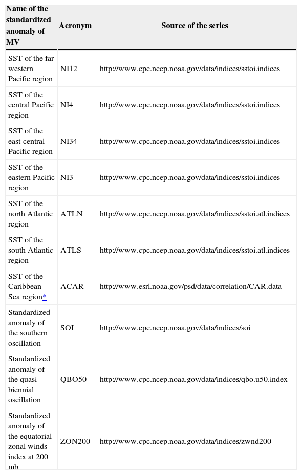
2.2.2Phase II. Lagged linear correlation analysis1. For the lagged correlation analysis, the standardized anomaly series of the macroclimate variables (MV) given in Table I were used as independent variables. The continuous rainfall series of the RS with no missing data was considered as the dependent variable.
Time series anomalies used in the lagged correlation analysis.
| Name of the standardized anomaly of MV | Acronym | Source of the series |
|---|---|---|
| SST of the far western Pacific region | NI12 | http://www.cpc.ncep.noaa.gov/data/indices/sstoi.indices |
| SST of the central Pacific region | NI4 | http://www.cpc.ncep.noaa.gov/data/indices/sstoi.indices |
| SST of the east-central Pacific region | NI34 | http://www.cpc.ncep.noaa.gov/data/indices/sstoi.indices |
| SST of the eastern Pacific region | NI3 | http://www.cpc.ncep.noaa.gov/data/indices/sstoi.indices |
| SST of the north Atlantic region | ATLN | http://www.cpc.ncep.noaa.gov/data/indices/sstoi.atl.indices |
| SST of the south Atlantic region | ATLS | http://www.cpc.ncep.noaa.gov/data/indices/sstoi.atl.indices |
| SST of the Caribbean Sea region* | ACAR | http://www.esrl.noaa.gov/psd/data/correlation/CAR.data |
| Standardized anomaly of the southern oscillation | SOI | http://www.cpc.ncep.noaa.gov/data/indices/soi |
| Standardized anomaly of the quasi-biennial oscillation | QBO50 | http://www.cpc.ncep.noaa.gov/data/indices/qbo.u50.index |
| Standardized anomaly of the equatorial zonal winds index at 200 mb | ZON200 | http://www.cpc.ncep.noaa.gov/data/indices/zwnd200 |
SST: Sea surface temperature.
2. The MVs given in Table I and the continuous rainfall series of each RS have different length of records; however, the common starting month is June 1979. A total of 23 RS with a minimum of 10 years of monthly common records were selected, and eight of these stations were discarded.
3. The SPI values for the selected RS are calculated for the common observation period of rainfall and MV anomalies.
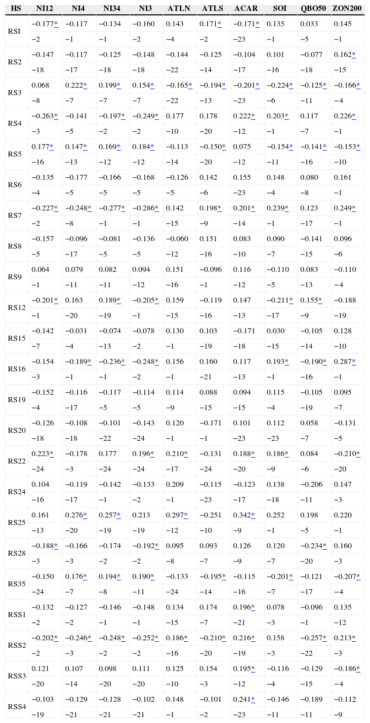
4. The Pearson correlation analysis between the SPI series in each RS and the MV anomalies given in Table I was applied. In the analysis, MV anomalies were lagged from 1 to 24 months with respect to the SPI series. For the correlation cases where the absolute value of Pearson coefficient reaches its maximum, the statistical significance of the correla tion coefficients is calculated. The results are given in Table II. As mentioned above, RS with less than 10 years of simultaneous common data of rainfall and MV anomalies were discarded.
Results of the Pearson correlation lagged analysis between SPI series in each RS and the MV anomalies.
| HS | NI12 | NI4 | NI34 | NI3 | ATLN | ATLS | ACAR | SOI | QBO50 | ZON200 |
|---|---|---|---|---|---|---|---|---|---|---|
| RSI | −0.177* | −0.117 | −0.134 | −0.160 | 0.143 | 0.171* | −0.171* | 0.135 | 0.033 | 0.145 |
| −2 | −1 | −1 | −2 | −4 | −2 | −23 | −1 | −5 | −1 | |
| RS2 | −0.147 | −0.117 | −0.125 | −0.148 | −0.144 | −0.125 | −0.104 | 0.101 | −0.077 | 0.162* |
| −18 | −17 | −18 | −18 | −22 | −14 | −17 | −16 | −18 | −15 | |
| RS3 | 0.068 | 0.222* | 0.199* | 0.154* | −0.165* | −0.194* | −0.201* | −0.224* | −0.125* | −0.166* |
| −8 | −7 | −7 | −7 | −22 | −13 | −23 | −6 | −11 | −4 | |
| RS4 | −0.263* | −0.141 | −0.197* | −0.249* | 0.177 | 0.178 | 0.222* | 0.203* | 0.117 | 0.226* |
| −3 | −5 | −2 | −2 | −10 | −20 | −12 | −1 | −7 | −1 | |
| RS5 | 0.177* | 0.147* | 0.169* | 0.184* | −0.113 | −0.150* | 0.075 | −0.154* | −0.141* | −0.153* |
| −16 | −13 | −12 | −12 | −14 | −20 | −12 | −11 | −16 | −10 | |
| RS6 | −0.135 | −0.177 | −0.166 | −0.168 | −0.126 | 0.142 | 0.155 | 0.148 | 0.080 | 0.161 |
| −4 | −5 | −5 | −5 | −5 | −6 | −23 | −4 | −8 | −1 | |
| RS7 | −0.227* | −0.248* | −0.277* | −0.286* | 0.142 | 0.198* | 0.201* | 0.239* | 0.123 | 0.249* |
| −2 | −8 | −1 | −1 | −15 | −9 | −14 | −1 | −17 | −1 | |
| RS8 | −0.157 | −0.096 | −0.081 | −0.136 | −0.060 | 0.151 | 0.083 | 0.090 | −0.141 | 0.096 |
| −5 | −17 | −5 | −5 | −12 | −16 | −10 | −7 | −15 | −6 | |
| RS9 | 0.064 | 0.079 | 0.082 | 0.094 | 0.151 | −0.096 | 0.116 | −0.110 | 0.083 | −0.110 |
| −1 | −11 | −11 | −12 | −16 | −1 | −12 | −5 | −13 | −4 | |
| RS12 | −0.201* | 0.163 | 0.189* | −0.205* | 0.159 | −0.119 | 0.147 | −0.211* | 0.155* | −0.188 |
| −1 | −20 | −19 | −1 | −15 | −16 | −13 | −17 | −9 | −19 | |
| RS15 | −0.142 | −0.031 | −0.074 | −0.078 | 0.130 | 0.103 | −0.171 | 0.030 | −0.105 | 0.128 |
| −7 | −4 | −13 | −2 | −1 | −19 | −18 | −15 | −14 | −10 | |
| RS16 | −0.154 | −0.189* | −0.236* | −0.248* | 0.156 | 0.160 | 0.117 | 0.193* | −0.190* | 0.287* |
| −3 | −1 | −1 | −2 | −1 | −21 | −13 | −1 | −16 | −1 | |
| RS19 | −0.152 | −0.116 | −0.117 | −0.114 | 0.114 | 0.088 | 0.094 | 0.115 | −0.105 | 0.095 |
| −4 | −17 | −5 | −5 | −9 | −15 | −15 | −4 | −19 | −7 | |
| RS20 | −0.126 | −0.108 | −0.101 | −0.143 | 0.120 | −0.171 | 0.101 | 0.112 | 0.058 | −0.131 |
| −18 | −18 | −22 | −24 | −1 | −1 | −23 | −23 | −7 | −5 | |
| RS22 | 0.223* | −0.178 | 0.177 | 0.196* | 0.210* | −0.131 | 0.188* | 0.186* | 0.084 | −0.210* |
| −24 | −3 | −24 | −24 | −17 | −24 | −20 | −9 | −6 | −20 | |
| RS24 | 0.104 | −0.119 | −0.142 | −0.133 | 0.209 | −0.115 | −0.123 | 0.138 | −0.206 | 0.147 |
| −16 | −17 | −1 | −2 | −1 | −23 | −17 | −18 | −11 | −3 | |
| RS25 | 0.161 | 0.276* | 0.257* | 0.213 | 0.297* | −0.251 | 0.342* | 0.252 | 0.198 | 0.220 |
| −13 | −20 | −19 | −19 | −12 | −10 | −9 | −1 | −5 | −1 | |
| RS28 | −0.188* | −0.166 | −0.174 | −0.192* | 0.095 | 0.093 | 0.126 | 0.120 | −0.234* | 0.160 |
| −3 | −3 | −2 | −2 | −8 | −7 | −9 | −7 | −20 | −3 | |
| RS35 | −0.150 | 0.176* | 0.194* | 0.190* | −0.133 | −0.195* | −0.115 | −0.201* | −0.121 | −0.207* |
| −24 | −7 | −8 | −11 | −24 | −14 | −16 | −7 | −17 | −4 | |
| RSS1 | −0.132 | −0.127 | −0.146 | −0.148 | 0.134 | 0.174 | 0.196* | 0.078 | −0.096 | 0.135 |
| −2 | −2 | −1 | −1 | −15 | −7 | −21 | −3 | −1 | −12 | |
| RSS2 | −0.202* | −0.246* | −0.248* | −0.252* | 0.186* | −0.210* | 0.216* | 0.158 | −0.257* | 0.213* |
| −2 | −3 | −2 | −2 | −16 | −20 | −19 | −3 | −22 | −3 | |
| RSS3 | 0.121 | 0.107 | 0.098 | 0.111 | 0.125 | 0.154 | 0.195* | −0.116 | −0.129 | −0.186* |
| −20 | −14 | −20 | −20 | −10 | −3 | −12 | −4 | −15 | −4 | |
| RSS4 | −0.103 | −0.129 | −0.128 | −0.102 | 0.148 | −0.101 | 0.241* | −0.146 | −0.189 | −0.112 |
| −19 | −21 | −21 | −21 | −1 | −2 | −23 | −11 | −11 | −9 |
Note: The upper value of each square is the maximum Pearson correlation coefficient; the bottom value indicates the lag in months where the maximum value of the Pearson correlation coefficient occurred (top line).
HS: Homogeneous sub-region.
1. In each RS, the four MV (predictor variables) with the highest degree of correlation were identified, as well as the associated lag. A database was structured so that each VM was shifted temporarily in connection with the SPI series, for as many months as the lag indicated in Table II.
2. Next, the MV series of Table I were grouped based on the location of each record in relation to quar-tiles Q2 and Q4, assigning them the following levels:
- •
−1: if VM ≤ Q2; negative signal
- •
0: if Q4 ≥ VM ≥ Q2; neutral signal
- •
+1: if VM ≥ Q4; positive signal
As indicated above, the SPI series are categorized as follows:
- •
SPI ≤ −2.00: month with an extremely dry condition (ED)
- •
−2.00 < SPI ≤ −1.50: month with a severely dry condition (SD)
- •
−1.50< SPI≤ −1.00: month with a moderately dry condition (MD)
- •
−1.00 ≤ SPI: month with a non-dry condition (ND)
3. With the three levels of the four predictor MV series and the four levels of SPI series, 81 possible combinations can be set in each RS. Furthermore, the probability of observed occurrence of ND, MD, SD, and ED conditions in each combination was calculated (total probability of Bayes [Cofiño, 2002; Evans, 2005]).
4. The models associated to each RS developed as indicated above were validated using 20 weather stations with continuous rainfall series operated by the Venezuelan Air Force. For the validation, the weather station located within the HS was selected and included in the GIS.
5. The homogeneity of the validation station series was verified by means of the statistical test of Easterling et al. (1996), using the AnClim software (Štěpánek, 2005). The corresponding SPI series were also categorized as follows:
- •
SPI ≤ −2.00: month with an ED condition
- •
−2.00 < SPI ≤ −1.50: months with an SD condition
- •
−1.50
- •
SPI ≤ −1.00: months with an ND condition
6. The validation level was established by calculating the percentage of right prediction successes with the RS models for the common period of validation station SPIs and predicted MVs. The prediction is considered a success when the model predicts a scenario (ED, SD, MD, ND) regardless of the associate percentage of occurrence; otherwise the success is labeled as a false alarm.
3Results and discussion3.1Regionalization of rainfall anomalies in VenezuelaThe spatial clustering of rainfall stations based on the factor given by the PCA allows the establishment of HSs, which differ from one another mainly in the total annual rainfall, and in a lesser extent in the occurrence of the dry season, the altitude and the proximity and orientation of the station with respect to the high mountain chains. A total of 32 HSs were identified in the north of Apure and Orinoco rivers, and only four in the rest of the country. Based on the spatial coverage of the HSs, droughts have a more homogeneous behavior over bigger areas on the southern facade than in the north face (Fig. 2). This could be an indication that the spatial homogeneity of droughts in the north of the country is affected by terrain geomorphology, height of the mountains units, leeside, and line-up of the sites in relation to the prevailing direction of trade winds (surface winds).

Comparing the Venezuelan climatic types (Koep-pen classification) with the distribution of HSs, there are analogies between the two patterns, especially in geographical areas with dry climates. Some HSs and areas with climates of the type BWI or BShi are overlapped as are the cases of Margarita Island and RS7, the bay of El Tablazo and RSI, Lara’s depression and SR8 (Fig. 2). On the contrary, there is not a clear association between climate type and the HSs in regions with warm rainy weather (Afi, Ami or Aw), as are the cases of Sierra of Maigualida, Brazo Casiquiare Penillanura or the southwest quadrant of Guayana Macizo, where the RS4 encompasses heterogeneous environments from the point of view of the amount and distribution of the annual rainfall. This differentiation could be explained by the fact that the physical mechanism that generates meteorological droughts (rainfall anomalies, in general) is more complex in humid regions than in those with a predominantly dry or arid weather, which are less affected by the double shift yearly occurrence of the Intertropical Convergence Zone (Goldbrunner, 1984; Pulwarty et al., 1992).
3.2Correlation analysis between SPI series of RS in each HS and anomalies of MVs for different monthly lagsResults of the correlation analysis between SPI and MV are given in Table II. The magnitude and sign of linear correlation, as well as the lag time between the SPI and the Pacific Ocean indexes NI12, NI4, NI34, and NI3, vary from one RS to another. In general, the higher correlation coefficients occur in the northeast flank of the country and in the western region (Zulia state). The same behavior can be observed in Table II for the Southern Oscillation Index (SOI). Although the ocean and atmosphere subsystems are coupled together, the dynamic of the physical phenomena differs, so that with a common start time they generate different responses according to the degree of lagging. The general circulation of the atmosphere takes only a few weeks, while the ocean circulation could be expanded for several years (Deza et al. 2003; Bobba and Minetti, 2010). Based on the above discussion, the SOI should be a better predictor variable for the rainfall anomalies (SPI) in each RS, in connection with the occurrence of the extreme ENSO phases (El Niño-La Niña). This fact justifies the consideration of this variable only for the development of the prediction models.
Results given in Table II show that the thermal anomalies in the Pacific and Atlantic oceans, the Caribbean Sea and the wind fields in the tropical upper troposphere and stratosphere, have a synergic effect on the precipitations in each HS. This fact is evident for the case of region RS25. Moreover, it could be inferred that oceanic and atmospheric signals of great magnitude, expressed in the form of anomalies, can be amplified, mitigated or canceled each other, demonstrating a complex interaction between the ocean and atmosphere subsystems, which in turn could be undergoing alterations by the global climate change.
3.3Structure and validation of predictive models in the homogeneous subregionsAs an example of predictive model development, the structure corresponding to the forecast model of HS and its reference station RSS3 (Fig. 2) will be described here. For this subregion the four mac-roclimatic indices that best correlate with the SPI of RSS3 are ACAR, ATLS, QBO50 and ZON200, whose correlation coefficients and corresponding monthly lags are 0.195, −12; 0.154, −3; −0.129, −15; and −0.186, −4, respectively. The common period of both series (SPI and selected MV) is from September 1980 to December 2001, with a total of 256 consecutive months.
Table III presents the quartiles of the four selected predictor variables and their corresponding lags with respect to SPI. The macroclimatic variable ATLS shows the highest correlation coefficient at lag −3 months, allowing a prognosis of three months in advance when using this variable.
The probability of occurrence of the above categorized dry events (ND, MD, SD, and ED) are given in Table IV for different structure combinations of the observed predictors and corresponding monthly lags (macroclimatic indices best correlated with the SPI of the RS in RSS3 as given in Table III).
Observed probability of occurrence for the given model structure and corresponding lag in the RS of RSS3 for the common period September 1980-December 2001.
| Model structure of MV predictor | Observed probability of occurrence (%) | ||||||
|---|---|---|---|---|---|---|---|
| ACAR | ATLS | QBO50 | ZON200 | ND | MD | SD | ED |
| −1 | −1 | 0 | 0 | 90.00 | 0.00 | 0.00 | 10.00 |
| −1 | −1 | 0 | 1 | 75.00 | 25.00 | 0.00 | 0.00 |
| −1 | −1 | 0 | −1 | 100.00 | 0.00 | 0.00 | 0.00 |
| −1 | −1 | −1 | −1 | 100.00 | 0.00 | 0.00 | 0.00 |
| −1 | −1 | 1 | 0 | 100.00 | 0.00 | 0.00 | 0.00 |
| −1 | 0 | 0 | 0 | 71.43 | 14.29 | 0.00 | 14.29 |
| −1 | 0 | 0 | 1 | 83.33 | 0.00 | 16.67 | 0.00 |
| −1 | 0 | −1 | 0 | 87.50 | 12.50 | 0.00 | 0.00 |
| −1 | 0 | −1 | 1 | 0.00 | 100.00 | 0.00 | 0.00 |
| −1 | 0 | −1 | −1 | 100.00 | 0.00 | 0.00 | 0.00 |
| −1 | 0 | 1 | 0 | 100.00 | 0.00 | 0.00 | 0.00 |
| −1 | 0 | 1 | 1 | 75.00 | 0.00 | 25.00 | 0.00 |
| −1 | 0 | 1 | −1 | 80.00 | 20.00 | 0.00 | 0.00 |
| −1 | 1 | 0 | 0 | 100.00 | 0.00 | 0.00 | 0.00 |
| −1 | 1 | 0 | 1 | 100.00 | 0.00 | 0.00 | 0.00 |
| −1 | 1 | 0 | −1 | 100.00 | 0.00 | 0.00 | 0.00 |
| −1 | 1 | −1 | 0 | 100.00 | 0.00 | 0.00 | 0.00 |
| −1 | 1 | 1 | 0 | 100.00 | 0.00 | 0.00 | 0.00 |
| 0 | −1 | 0 | 0 | 66.67 | 22.22 | 0.00 | 11.11 |
| 0 | −1 | 0 | 1 | 100.00 | 0.00 | 0.00 | 0.00 |
| 0 | −1 | 0 | −1 | 100.00 | 0.00 | 0.00 | 0.00 |
| 0 | −1 | −1 | 0 | 25.00 | 0.00 | 50.00 | 25.00 |
| 0 | −1 | −1 | −1 | 100.00 | 0.00 | 0.00 | 0.00 |
| 0 | −1 | 1 | 0 | 100.00 | 0.00 | 0.00 | 0.00 |
| 0 | −1 | 1 | 1 | 100.00 | 0.00 | 0.00 | 0.00 |
| 0 | −1 | 1 | −1 | 100.00 | 0.00 | 0.00 | 0.00 |
| 0 | 0 | 0 | 0 | 85.71 | 0.00 | 14.29 | 0.00 |
| 0 | 0 | 0 | 1 | 90.91 | 9.09 | 0.00 | 0.00 |
| 0 | 0 | 0 | −1 | 100.00 | 0.00 | 0.00 | 0.00 |
| 0 | 0 | −1 | 0 | 87.50 | 12.50 | 0.00 | 0.00 |
| 0 | 0 | −1 | −1 | 80.00 | 20.00 | 0.00 | 0.00 |
| 0 | 0 | 1 | 0 | 91.67 | 0.00 | 8.33 | 0.00 |
| 0 | 0 | 1 | 1 | 100.00 | 0.00 | 0.00 | 0.00 |
| 0 | 0 | 1 | −1 | 75.00 | 25.00 | 0.00 | 0.00 |
| 0 | 1 | 0 | 0 | 70.00 | 30.00 | 0.00 | 0.00 |
| 0 | 1 | 0 | 1 | 80.00 | 20.00 | 0.00 | 0.00 |
| 0 | 1 | 0 | −1 | 100.00 | 0.00 | 0.00 | 0.00 |
| 0 | 1 | −1 | 0 | 100.00 | 0.00 | 0.00 | 0.00 |
| 0 | 1 | −1 | −1 | 100.00 | 0.00 | 0.00 | 0.00 |
| 0 | 1 | 1 | 0 | 100.00 | 0.00 | 0.00 | 0.00 |
| 0 | 1 | 1 | −1 | 100.00 | 0.00 | 0.00 | 0.00 |
| 1 | −1 | 0 | 1 | 100.00 | 0.00 | 0.00 | 0.00 |
| 1 | −1 | −1 | 0 | 100.00 | 0.00 | 0.00 | 0.00 |
| 1 | −1 | −1 | 1 | 100.00 | 0.00 | 0.00 | 0.00 |
| 1 | −1 | 1 | 0 | 100.00 | 0.00 | 0.00 | 0.00 |
| 1 | 0 | 0 | 0 | 100.00 | 0.00 | 0.00 | 0.00 |
| 1 | 0 | 0 | 1 | 62.50 | 37.50 | 0.00 | 0.00 |
| 1 | 0 | 0 | −1 | 100.00 | 0.00 | 0.00 | 0.00 |
| 1 | 0 | −1 | 0 | 100.00 | 0.00 | 0.00 | 0.00 |
| 1 | 0 | −1 | 1 | 100.00 | 0.00 | 0.00 | 0.00 |
| 1 | 0 | 1 | 1 | 100.00 | 0.00 | 0.00 | 0.00 |
| 1 | 1 | 0 | 0 | 100.00 | 0.00 | 0.00 | 0.00 |
| 1 | 1 | 0 | 1 | 100.00 | 0.00 | 0.00 | 0.00 |
| 1 | 1 | 0 | −1 | 100.00 | 0.00 | 0.00 | 0.00 |
| 1 | 1 | −1 | 0 | 100.00 | 0.00 | 0.00 | 0.00 |
| 1 | 1 | −1 | 1 | 100.00 | 0.00 | 0.00 | 0.00 |
| 1 | 1 | −1 | −1 | 100.00 | 0.00 | 0.00 | 0.00 |
| 1 | 1 | 1 | 0 | 100.00 | 0.00 | 0.00 | 0.00 |
| 1 | 1 | 1 | 1 | 100.00 | 0.00 | 0.00 | 0.00 |
Note: This table shows only observed combinations.
A simplified flow diagram to organize the seasonal drought forecast weather is given in Figure 3.

Its routine forecast comprises the following steps:
- 1.
The user selects the HS where the forecast is required, e.g. RSS3 (Apure).
- 2.
The system identifies the four MV predictors of the SH of interest (for the example given in Table III, these will be ACAR, ATLS, QBO50 and ZON200). The information is retrieved from a database that contains the data of all MV predictors for each HS.
- 3.
The system identifies the corresponding monthly lag of each MV predictor in the HS of interest. For the example in Table III, the values will be −12, −3, −15, and −4, for ACAR, ATLS, QBO50, and ZON200, respectively.
- 4.
The system identifies and reads the quartiles Q2 and Q4 of each predictor MV in the HS of interest. This information is part of the database (an example is given in Table III).
- 5.
The system reads the anomalies of the predictor MV properly lagged in the HS of interest. This information should be contained in a database updated monthly using the original sources of the anomalies series: ACAR, ATLS, QBO50, and ZON200. Returning to the example and assuming that it is necessary to predict the condition prevailing in the RSS3 on May 2011, the lagged anomalies will be 0.375 (ACAR), 0.450 (ATLS), 0.070 (QBO50), and 2.600 (ZON200).
- 6.
The system transforms each of the mentioned anomalies in a ternary numeric value: −1, 0 or +1, according to the position of the measure value compared with the quartiles Q2and Q4.
- 7.
The system determines the structure of the input signal, using the values from the previous step. A signal has four whole numbers (one for each predictor MV) and the ternaries. In our example, the input signal is +1, +1, 0, +1.
- 8.
The system searches the code from the previous step in the structures contained in the HS model. If the code is part of the HS model, the user is informed about the observed probability of occurrence of a given dry condition (ND, MD, SD, ED) for the tested month. If the code is not contained in the HS model (not observed during the period when the predictor MV series and the SPI are contrasted), the user is warned that the system cannot emit a forecast. In the example, the forecast probability for May 2011 in SRS3 is 100.00% (ND), 0.00% (MD), 0.00% (SD), and 0.00% (ED).
The validation analysis of the model shows a good level of prediction accuracy for the occurrence of ED events with success rates higher than 85.2%. In general, the percentage of right answers is directly proportional to the length of the observation period considered in the development of the model structure (as given in Table IV). Apparently the geographic location of the RSs (north or south facade) does not seem to influence the percentage of right answers when applying the models. The weather events with ND and MD conditions have the highest percentage of false alarms (around 21.16%); this suggests that, as a result of the way in which the model is generated, it does not discern adequately the occurrence of these events.
4ConclusionsWeather stations in Venezuela are regionalized according to the magnitude and sign of rainfall anomalies expressed by the SPI index. PCA with standard Varimax rotation and Kaiser normalization allows identifying the stations with interrelated SPI that form groups with a high degree of homogeneity.
The use of a GIS to represent those groups allows defining continuous geographic regions, the so-called HS. Gauging stations included in an HS region can be represented by an RS selected on the base of record length, occurrence of the dry season, altitude, and annual mean precipitation. The generated homogeneous groups are of different sizes. The first component comprises the largest number of stations. The mean annual rainfall and, in a lesser degree, the orientation of the stations in relation to the mountain barriers appear to influence the formation of the HSs.
Extreme temperature anomalies in the Pacific (El Niño regions), the North and South Atlantic and the Caribbean Sea have a differential effect on the occurrence of precipitation in Venezuela. These macroclimatic weather events alter temporarily the total normal rainfall, and may also change the spatial distribution pattern of rainfall on a regional scale. Between the occurrence of an oceanic or atmospheric anomaly and the occurrence of the resulting extreme rainfall event, there is a lag time of 1 to 23 months. Under certain conditions the occurrence of meteorological droughts is modulated by the changes in the pattern and intensity of air circulation in the tropical upper troposphere and stratosphere. The droughts of greater spatial coverage and persistence are the result of the interaction of several macroclimatic anomalies of different magnitude, sign, origin (oceanic or atmospheric), and time lag.
The developed predictive models based on the use of conditional probability tables allow predicting with an accuracy of more than 60% the occurrence of ED events in several areas of the country with an anticipation of one to 14 months. To minimize the uncertainty of the forecast, the RS should have a rainfall series with an extended length of rainfall records.
The structure of the proposed model is easy to program and only requires continuous records of monthly precipitation; therefore, it should be easy to incorporate this model into an early warning system for drought weather (SATSM) in Venezuela or any other country where teleconnections play an important role in the occurrence of extreme rainfall anomalies.
Unlike the complex coupled general circulation atmosphere-ocean models, the proposed method uses simple algorithms and is easy to program, so it can easily be adapted to any Latin American country and the Caribbean regions, provided that there is enough rainfall data available.
This work was developed in the Centro de Investigaciones Hidrológicas y Ambientales, Universidad de Carabobo, and was funded by the Consejo para el Desarrollo Científico y Humanístico of the same institution and the Grupo para Investigaciones sobre Cuencas Hidrográficas y Recursos Hidráulicos, Coordinación de Investigación, VIPI-UNELLEZ, San Carlos, Cojedes state.