


The performance of diagnostic tests can be assessed by a number of methods. These include sensitivity, specificity, positive and negative predictive values, likelihood ratios and receiver operating characteristic (ROC) curves. This paper describes the methods and explains which information they provide. Sensitivity and specificity provides measures of the diagnostic accuracy of a test in diagnosing the condition. The positive and negative predictive values estimate the probability of the condition from the test-outcome and the condition’s prevalence. The likelihood ratios bring together sensitivity and specificity and can be combined with the condition’s pre-test prevalence to estimate the posttest probability of the condition. The ROC curve is obtained by calculating the sensitivity and specificity of a quantitative test at every possible cut-off point between ‘normal’ and ‘abnormal’ and plotting sensitivity as a function of 1-specificity. The ROC-curve can be used to define optimal cut-off values for a test, to assess the diagnostic accuracy of the test, and to compare the usefulness of different tests in the same patients. Under certain conditions it may be possible to utilize a test’s quantitative information as such (without dichotomization) to yield diagnostic evidence in proportion to the actual test value. By combining more diagnostic tests in multivariate models the diagnostic accuracy may be markedly improved.
The performance of diagnostic tests can be assessed by a number of methods developed to ensure the optimal utilization of the information provided by symptoms, signs and investigational tests of any kind for the benefit of the patient. The evaluations of diagnostic tests include sensitivity, specificity, positive and negative predictive values, likelihood ratios and ROC-curves.1 This article will review these methods and provide some suggestions for their extension and improvement. The methods will be illustrated by an important variable in hepatology, namely the hepatic venous pressure gradient (HVPG).
The decision of the doctor in regard to diagnosis and therapy is based on the variables characterising the patient. It is therefore essential for the doctor: a) to know which variables hold the most information and b) to be able to interpret the information in the best possible way.1 How this is done depends on the type of the variable and on the type of decision, which has to be made. Some descriptive variables are by nature dichotomous or binary like variceal bleeding being either present or absent. However, many variables like liver function tests and the hepatic venous pressure gradient (HVPG) are measured on a continuous scale, i.e. they are quantitative variables.
A doctor’s decision has to be binary, i.e. yes or no concerning a specific diagnosis and treatment. Therefore, for a the simple diagnostic tests to provide a yes or no answer, quantitative variables need to be made binary by introducing a threshold or cut-off level to distinguish between ‘normal’ and ‘abnormal’ values.
Classification of ‘Normal’ and ‘Abnormal’Most diagnostic tests would not be able to distinguish completely between ‘normal’ and ‘abnormal’; usually some overlap of varying degree would be present between the two categories. The overlap causes some patients to be misclassified. The larger the overlap, the poorer the discrimination of the test and the larger the proportion of misclassified patients. This is illustrated in figure 1. Patients with the condition in question (here variceal bleeding) could have a positive test (here hepatic venous pressure gradient (HVPG) above 12 mm Hg). They would be the True Positives (TP). But some patients with the condition could have a negative test i.e. an HPVG below 12 mm Hg. They would be the False Negatives (FN). In patients without the condition, the test would frequently be negative i.e. the HVPG would be below 12 mm Hg. That would the True Negatives (TN). But some patients without the condition could have a positive test i.e. an HVPG above 12 Hg. That would be the False Positives (FP). The false negatives and the false positives are the patients who are misclassified. An effective diagnostic test would only misclassify few patients.
 in patients without variceal bleeding and in patients with variceal bleeding. Since the distributions overlap, the HVPG does not provide complete discrimination between bleeding and non-bleeding patients. For most of the patients with variceal bleeding the HVPG would be above the discrimination threshold (usually 12 mm Hg); they would be classified as True Positives (TP). However, some patients with variceal bleeding would have HVPG below the discrimination threshold; they would be classified as False Negatives (FN). For most of the patients without variceal bleeding the HVPG would be below the discrimination threshold of 12 mm Hg; they would be classified as True Negatives (TN). However, some patients without variceal bleeding would have HVPG above the discrimination threshold; they would be classified as False Positives (FP).")
Schematic illustration of the distribution of HVPG (hepatic venous pressure gradient) in patients without variceal bleeding and in patients with variceal bleeding. Since the distributions overlap, the HVPG does not provide complete discrimination between bleeding and non-bleeding patients. For most of the patients with variceal bleeding the HVPG would be above the discrimination threshold (usually 12 mm Hg); they would be classified as True Positives (TP). However, some patients with variceal bleeding would have HVPG below the discrimination threshold; they would be classified as False Negatives (FN). For most of the patients without variceal bleeding the HVPG would be below the discrimination threshold of 12 mm Hg; they would be classified as True Negatives (TN). However, some patients without variceal bleeding would have HVPG above the discrimination threshold; they would be classified as False Positives (FP).
The classification of the patients by the test can be summarized in a 2 x 2 table as shown in table 1.
Test classification of patients summarized in a 2 × 2 table. The example shows the relation between high (< 12 mm Hg) or low (≥ 12 mm Hg) Hepatic Venous Pressure Gradient (HVPG) and occurrence of variceal bleeding.
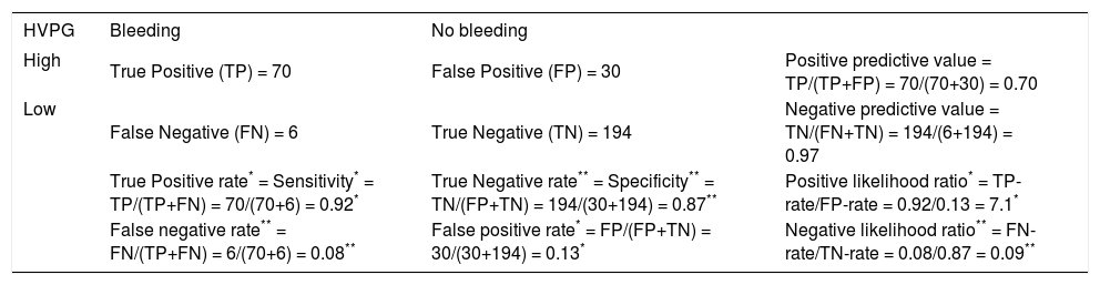
The performance of a binary classification test can be summarized as the sensitivity and specificity2-4 (Table 2).
Various measures of performance of a binary classification test. In this table the example presented in table 1 is supplemented by the definition and calculation of sensitivity (true positive rate), false positive rate, positive likelihood ratio (*), specificity (true negative rate), false negative rate, negative likelihood ratio (**), positive predictive value and negative predictive value.
| HVPG | Bleeding | No bleeding | |
|---|---|---|---|
| High | True Positive (TP) = 70 | False Positive (FP) = 30 | Positive predictive value = TP/(TP+FP) = 70/(70+30) = 0.70 |
| Low | False Negative (FN) = 6 | True Negative (TN) = 194 | Negative predictive value = TN/(FN+TN) = 194/(6+194) = 0.97 |
| True Positive rate* = Sensitivity* = TP/(TP+FN) = 70/(70+6) = 0.92* | True Negative rate** = Specificity** = TN/(FP+TN) = 194/(30+194) = 0.87** | Positive likelihood ratio* = TP-rate/FP-rate = 0.92/0.13 = 7.1* | |
| False negative rate** = FN/(TP+FN) = 6/(70+6) = 0.08** | False positive rate* = FP/(FP+TN) = 30/(30+194) = 0.13* | Negative likelihood ratio** = FN-rate/TN-rate = 0.08/0.87 = 0.09** |
- •
The sensitivity measures the proportion of actual positives, which are correctly identified as such. It is also called the true positive rate. In the example in table 2 the sensitivity or true positive rate is the probability of high HVPG in patients with bleeding.
- •
The specificity measures the proportion of actual negatives, which are correctly identified as such. It is also called the true negative rate. In the example the specificity or true negative rate is the probability of low HVPG in patients with no bleeding.
A sensitivity (true positive rate) of 100% means that the test classifies all patients with the condition correctly. A negative test-result can thus rule out the condition.
A specificity (true negative rate) of 100% means that the test classifies all patients without the condition correctly. A positive test-result can thus confirm the condition.
Complementary to the sensitivity is the false negative rate, i.e. it is equal to 1 - sensitivity. This is sometimes also called the type 2 error (ß), which is the risk of overlooking a positive finding when it is in fact true. In the example used the false negative rate is the probability of bleeding in patients with low HVPG.
Complementary to the specificity is the false positive rate, i.e. it is equal to 1 - specificity. This is sometimes also termed the type 1 error (a), which is the risk of recording a positive finding when it is in fact false. In the example the false positive rate is the probability of no bleeding in patients with high HVPG.
Positive and negative predictive valuesThe weaknesses of sensitivity and specificity are: a) that they do not take the prevalence of the condition into consideration and b) that they just give the probabilities of test-outcomes in patients with or without the condition. The doctor needs the opposite information, namely the probabilities of the condition in patients with a positive or negative test-outcome, i.e. the positive predictive value and negative predictive value4-5 defined below (Table 2).
- •
The positive predictive value (PPV) is the proportion of patients with positive test results who are correctly diagnosed as having the condition. It is also called the post-test probability of the condition. In the example the positive predictive value (PPV) is the probability of bleeding in patients with high HVPG.
- •
The negative predictive value (NPV) is the proportion of patients with negative test results who are correctly diagnosed as not having the condition. In the example the negative predictive value (NPV) is the probability of no bleeding in patients with low HVPG.
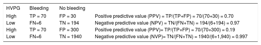
Both the positive and negative predictive values depend on the prevalence of the condition with may vary from place to place. This is illustrated in table 3. With decreasing prevalence of the condition the positive predictive value (PPV) decreases and the negative predictive value (NPV) increases - conversely with increasing prevalence of the condition.
Table 3..Example showing the influence of a lower prevalence of variceal bleeding on the positive and negative predictive values. By increasing the prevalence of bleeding from 25% (upper panel) to 3.3% (lower panel) the positive predictive value (PPV) decreases from 0.70 to 0.19 and the negative predictive value (NPV) increases from 0.97 to 0.997.
HVPG Bleeding No bleeding High TP = 70 FP = 30 Positive predictive value (PPV) = TP/(TP+FP) = 70/(70+30) = 0.70 Low FN=6 TN = 194 Negative predictive value (NPV) = TN/(FN+TN) = 194/(6+194) = 0.97 High TP = 70 FP = 300 Positive predictive value (PPV)= TP/(TP+FP) = 70/(70+300) = 0.19 Low FN=6 TN = 1940 Negative predictive value (NVP)= TN/(FN+TN) = 1940/(6+1,940) = 0.997
A newer tool of expressing the strength of a diagnostic test is the likelihood ratio, which incorporates both the sensitivity and specificity of the test and provides a direct estimate of how much a test result will change the odds of having the condition.6-8
- •
The likelihood ratio for a positive result (LR+) tells you how much the odds of the condition increase when the test is positive.
- •
The likelihood ratio for a negative result (LR-) tells you how much the odds of the condition decrease when the test is negative.
Table 2 shows how the likelihood ratios are being calculated using our example. The positive likelihood ratio (LR+) is the ratio between the true positive rate and the false positive rate. In our example it is the probability of high HVPG among bleeders divided by the probability of high HVPG among non-bleeders.
The negative likelihood ratio (LR-) is the ratio between the false negative rate and the true negative rate. In the example it is the probability of low HVPG among bleeders divided by the probability of low HVPG among non-bleeders.
The advantages of likelihood ratios are:
- •
That they do not vary in different populations or settings because they are based on ratio of rates.
- •
They can be used directly at the individual level.
- •
They allow the clinician to quantitate the probability of bleeding for any individual patient.
- •
Their interpretation is intuitive: i.e. the larger the LR+, the greater the likelihood of bleeding, the smaller the LR-, the lesser the likelihood of bleeding.
Likelihood ratios can be used to calculate the post-test probability of the condition using Bayes’ theorem, which states that the post-test odds equals the pre-test odds times the likelihood ratio: Post-test odds = pre-test odds × likelihood ratio.7,9
Using our example (Table 2) we can now calculate the probability of bleeding with high HVPG using LR+ as follows: The pre-test probability p1 (or prevalence) of bleeding is 0.25. The pre-test probability p2 (or prevalence) of no bleeding is thus 1-0.25 = 0.75. The pre-test odds of bleeding/no bleeding = p1/ p2 = 0.25/0.75 = 0.34. Since LR+ = 6.9 we can (using Bayes’ theorem) calculate the post-test odds o1 as 0.34 x 6.9 = 2.34. Then we can calculate the post-test probability of bleeding with a high HVPG as o1/(1+ o1) = 2.34/3.34 = 0.70. Note that this is the same value as the PPV.
Similarly we can calculate the probability of bleeding with a low HVPG using LR-as follows: As before the pre-test odds of bleeding/no bleeding is 0.34. Since the LR- = 0.09 the post-test odds o2 = 0.34 x 0.09 = 0.03. Then the post-test probability of bleeding with a low HVPG is o2/(1+ o2) = 0.03/ 1.03 = 0.03. Note that this is the same value as 1-NPV. The calculation of post-test probabilities from pre-test probabilities and likelihood-ratios is greatly facilitated using a nomogram.10
The Role Of The Discrimination ThresholdThe specification of the discrimination threshold or cut-off is important for the optimal performance of a diagnostic test based on a quantitative variable test like the HVPG. As the position of the threshold changes, the sensitivity and the specificity also change. If you want a high sensitivity (true positive rate), you would specify a relatively low discrimination threshold. If you want a high sensitivity (true negative rate) you would specify a relatively high discrimination threshold. The effect of changing the position of the discrimination threshold is illustrated in figure 2 (left side) together with the receiver operating characteristic (ROC) curve (Figure 2, right side), which summarizes the overall performance of a diagnostic test.11-14 The ROC curve shows the true positive rate (sensitivity) as a function of the false positive rate (1 - specificity) as the discrimination threshold runs through all the possible values.
 and the position on the receiver operating characteristic (ROC) curve (B). The ROC curve is a graphical plot of the true positive rate (sensitivity) as a function of the false positive rate (1-specificity) for a diagnostic test as its discrimination threshold is varied through the whole range. By moving the discrimination threshold from left to right, the points on the ROC curve are obtained from right to left. The figure shows the correspondence between three positions of the discrimination threshold (A) and the three corresponding points on the ROC curve (B).")
The relation between the discrimination threshold (A) and the position on the receiver operating characteristic (ROC) curve (B). The ROC curve is a graphical plot of the true positive rate (sensitivity) as a function of the false positive rate (1-specificity) for a diagnostic test as its discrimination threshold is varied through the whole range. By moving the discrimination threshold from left to right, the points on the ROC curve are obtained from right to left. The figure shows the correspondence between three positions of the discrimination threshold (A) and the three corresponding points on the ROC curve (B).
The degree of separation between two distributions is given by the discriminability index d’, which is the difference in means of the two distributions divided by their standard deviation.15Figure 3 shows that with increasing separation (decreased overlap) between the distributions the discriminability index increases (Figure 3, left side) and the middle of the ROC curve moves up toward the upper left corner of the graph (Figure 3, right side). For the discriminability index to be valid, the distributions need to be normal with similar standard deviations. In practice these requirements may not always be fulfilled.
 between the test distribution curves for patients with (dsicontinuous line) or without (continuous line) the condition a) on the discriminability index (A) and b) on the position of the ROC curve (B).")
The area under the ROC curve (AUC) or c-statistic is another measure of how well a diagnostic test performs (Figure 4).11-14 With increasing discrimination between the test distributions for patients with and without the condition, the AUC or c-statistic will increase. An AUC of 0.5 means no discrimination, an AUC = 1 means perfect discrimination. Most frequently the AUC or c-statistic would lie in the interval 0.7-0.8. The standard error of an AUC can be calculated and ROC-curves for different diagnostic tests derived from the same patients can be compared statistically.16-18 In this way the test with the highest diagnostic accuracy in the patients can be found.
 or c-statistic. The better the discrimination, the larger the AUC or c-statistic. An AUC of 0.5 means no discrimination, an AUC = 1 means perfect discrimination.")
The ROC-curve can also be used to define the optimal cut-off value for a test by localizing the value where the overall misclassification (false positive rate plus false negative rate) is minimum. This will usually be the cut-off value corresponding to the point of the ROC curve, which is closest to upper left corner of the plot (i.e. point [0, 1]).
The performance of diagnostic tests may be improved if ‘noise’ in the measurement of the diagnostic variable e.g. HVPG can be reduced as much as possible. Therefore every effort should be made to reduce the influence of factors, which could make the measurements less accurate. Thus if ‘noise’ can be reduced, the spread of the test distributions would be less, the test distributions would be narrower with less overlap, and this would improve the test’s discrimination between those with and those without the condition.
Weaknesses Of DichotomizationThe preceding methods of utilizing the information provided by a quantitative diagnostic variable like HVPG involve dichotomization defining ‘normal’ and ‘abnormal’. Thus the quantitative information provided by the test-value within each of the two defined groups (normal or abnormal) is not utilized. All test-values smaller than the cutoff are considered equal and all test-values larger than the cutoff are also considered equal. By disregarding the actual value of the test-variable within each of the groups (normal, abnormal) information is lost.
Strength Of Evidence Based On Test-ValueIn the following a method utilizing quantitative test-values as such without dichotomization will be described. Considering the HVPG there would be a relation between the risk of bleeding and the actual level of HVPG irrespective any defined threshold: the smaller the HVPG, the lesser the risk of bleeding; the larger the HVPG, the greater the risk of bleeding.
The risk can be expressed as the likelihood ratio (the ratio between the probability densities or heights) of the two distribution curves at the actual HVPG level (Figure 5).19 From the likelihood ratio and the pre-test probability of bleeding the post-test probability of bleeding can be estimated using Bayes’ theorem as shown previously in this paper. However, this likelihood ratio method would only be valid if the distribution curves for bleeding and non-bleeding were normal with the same standard deviation. These requirements may not be entirely fulfilled in practice. If they are not fulfilled it may be possible to perform a normalizing transformation of the variable or to perform analysis after dividing the information of the quantitative variable into a smaller number of groups e.g. 3 or 4 groups.
 of the two distribution curves for variceal bleeding and no bleeding at the actual HVPG level. For this procedure to be valid both distribution curves should be normal and have the same standard deviation. In example 1 the likelihood ratio of bleeding to no bleeding is 0.5 since the height (a) up to the curve for variceal bleeding is only half the height (b) up to the curve for no bleeding. In example 2 the likelihood ratio of bleeding to non-bleeding is 0.12 since the height (z) up to the curve for variceal bleeding is only 0.12 of the height (w) up to the curve for non-bleeding. Thus for a given patient the risk of bleeding can be estimated from his/her actual HVPG level.")
Likelihood ratio based on probability densities (heights) of the two distribution curves for variceal bleeding and no bleeding at the actual HVPG level. For this procedure to be valid both distribution curves should be normal and have the same standard deviation. In example 1 the likelihood ratio of bleeding to no bleeding is 0.5 since the height (a) up to the curve for variceal bleeding is only half the height (b) up to the curve for no bleeding. In example 2 the likelihood ratio of bleeding to non-bleeding is 0.12 since the height (z) up to the curve for variceal bleeding is only 0.12 of the height (w) up to the curve for non-bleeding. Thus for a given patient the risk of bleeding can be estimated from his/her actual HVPG level.
Besides the key variable HVPG other descriptive variables (e.g. symptoms, signs and liver function tests) may influence the risk of bleeding from varices. By utilizing such additional information, estimation of the risk of bleeding in a given patient may be improved. Such predictive models may be developed using multivariate statistical analysis like logistic regression or Cox regression analysis.20,21
In the literature there are many examples of utilizing the combined diagnostic information of more variables.22,23 Here will just be mentioned one example by Merkel, et al. who showed that the prediction of variceal bleeding could be improved by supplementing the information provided by HVPG with information of the Pugh score, the size of the esophageal varices and whether variceal bleeding had occurred preciously.24 Their multivariate model had significantly more predictive power than HVPG alone.
ConclusionThe methods for evaluation of simple diagnostic tests provided in this paper are important tools for optimal evaluation of patients. They may, however, have limitations for quantitative variables, since the dichotomization, which needs to be made, has the consequence that quantitative information is being lost. Quantitative variables should be kept as such whenever possible. Prediction of diagnosis and outcome may be markedly improved if more informative variables can be combined using multivariate statistical analysis e.g. logistic regression analysis. Preferably dichotomization of quantitative variables should only be used in the last step, when a binary decision (i.e. yes/no in regard to diagnosis or therapy) has to be made.