


The behavioral agent-based framework of De Grauwe and Gerba (2015) is extended to allow for a counterfactual exercise on the role of corporate finance arrangements for monetary transmission. Two alternative firm financial frictions are independently introduced: market-based and bank-based. We find convincing evidence that the overall monetary transmission channel is stronger in the bank-based system compared to the market-based. While the growth in credit is larger in the market-based system, uncertainty originated from imperfect beliefs produce impulse responses in macroeconomic variables that are, on average, half of those in the bank-based model. At the same time we find mixed results on the conditional effectiveness of monetary policy to offset contractions. Conditional on being in a recession, a monetary expansion in a market-based system creates higher successive booms. That said, a monetary easing in the bank-based system is more effective in smoothening the financial-and business cycles.
El modelo de comportamiento basado en agentes de De Grauwe y Gerba (2015) se extiende para permitir un ejercicio contrafactual del papel que desempeñan los acuerdos financieros corporativos para la transmisión monetaria. Se analizan de manera independiente dos fricciones financieras alternativas sobre las firmas: la basada en el mercado y la basada en la banca. Se encuentran pruebas convincentes de que el canal de transmisión monetaria en su conjunto es más fuerte en el sistema basado en la banca que aquel basado en el mercado. Si bien crece más el crédito en el sistema basado en el mercado, la incertidumbre generada por las creencias imperfectas produce impulsos respuesta en las variables macroeconómicas que son, en promedio, la mitad de las del modelo basado en la banca. Al mismo tiempo, se encuentran resultados mixtos en la eficacia condicional de la política monetaria para contarrestar las contracciones. Bajo la condición de encontrarse en una recesión, una expansión monetaria dentro de un sistema basado en el mercado crea unos auges sucesivos mayores. Dicho esto, la expansión monetaria es más eficaz en el sistema basado en la banca a la hora de suavizar los ciclos financiero y económico.
There is a long line of empirical research highlighting a strong link between firm characteristics, corporate finance structure and monetary policy transmission. Those studies show that the effectiveness of monetary policy and the asymmetric impact it will have on the economy over expansions vs recessions is dependent on the type of firms in the economy and their financing composition. Under the current context of unconventional policies understanding this link has become even more urgent. Despite the enormous amount of liquidity injected by central banks, SMEs continue to face many difficulties to access credit. This is true for both the UK and Euro Area (EA). For others, such as the US these difficulties have been much less acute. For emerging markets, access to firm credit is still very problematic despite largely using conventional monetary policy tools. Yet, all these countries have very different corporate financing systems, and their central banks have adopted very different monetary policy. At the same time, their markets are at very different levels of market confidence. For this reason it is important to understand the interaction between monetary policy, market sentiments and credit supply, and examine whether the observed disparity in monetary policy effectiveness to boost credit and economic activity depends on the type of financial frictions in an economy.
We incorporate these components in our analysis and examine the role of monetary policy in boosting activity under competing financial regimes. In particular, we focus on two alternatives: one where firms receive external finances from the market market-based financing or MBF), and another where they receive it from banks (bank-based financing or BBF). We include each regime in separate but otherwise identical New-Keynesian models with price rigidities, a borrowing constraint for firms, financial frictions on the supply side and imperfect credit and capital markets. Borrowing constraint of firms has significant aggregate effects via the usual demand-channel, but also a more elaborated supply-channel via imperfect capital markets. In each version, firms can only access one type of external finance. This assumption makes the model more tractable and assists in making our key findings more understandable at the expense of making it somewhat less realistic. Further, we relax the rational expectations assumption and introduce behavioral dynamics of De Grauwe (2011) and De Grauwe and Gerba (2015).
Using the models, we wish to answer a number of questions. First, we wish to structurally uncover whether the source of corporate credit and the type of credit channel matters for monetary transmission. Second, we wish to examine the role of imperfect beliefs and stock markets for credit- and business cycle fluctuations. Finally, our ultimate aim is to answer a broader (long-standing) issue of whether monetary policy is more effective in generating and sustaining booms in a MBF or a BBF system. In other words, is the transmission of monetary policy to firm credit greater and smoother in one financial system compared to the other. This debate is nested within a larger contemporary debate of whether MBF systems cause larger economic instability and make monetary policy less effective in counteracting those. Therefore, by comparing two alternative yet pure financial regimes, we wish to highlight the contribution of each to economic (in)stability, and effectively examine the role that monetary policy has to play for relaxing credit access and smoothen business cycle fluctuations. Moreover, in the context of emerging markets, we hope that our findings will contribute to the debate of whether these should adopt market-based financing structure in order to relax credit access to firms, boost growth and improve the workings of monetary policy.
In the impulse response analysis, we find that a credit boom caused by a monetary expansion is stronger in a market-based system. The interaction between the actual drop in interest rate with positive market outlook relaxes the credit constraint more than proportionally. That said, the impulse response estimates in the MBF version are much wider which implies that there is a non-negligible probability of the credit expansion being smaller than in the BBF version. It mainly depends on the strength of the initial animal spirit channel.
The macroeconomic effects from this expansion, on the other hand, are stronger in the bank-based version. This is because less of the market uncertainty is passed through to the real economy, which allows it to expand more. In some sense, the marginal benefit of a unit of credit is higher in a bank-based financing system.
Interactions between market beliefs and financial frictions can potentially generate high amplitudes in the financial and business cycles. Longer expansions are followed by even deeper recessions. The heavy contractions are observed in standard macroeconomic as well as financial variables. In addition, cycles are asymmetric around the zero-line. Compared to rational expectations models, this is possible to generate because of the additional uncertainty (or friction) originating from imperfect beliefs.
One level down, these fluctuations (and asymmetries) are higher for financial variables in the BBF, while they are higher for macroeconomic variables in the MBF. This means that even if the additional banking friction in the BBF model generates greater fluctuations in the credit variables, the pass-through to the real economy is smoother. Banks absorb some of that volatility using their capital buffers. In the MBF version, on the other hand, that volatility is directly passed on to borrowers, who include them in their intertemporal decision-making.
To conclude, we evaluate the effect of monetary expansions conditional on the economy being in a recession. While interest rate cuts are more frequent and larger in the BBF model, the total effect on output is more modest. Capital restrictions and the limited influence of market sentiment in loan supply decisions limit the full-fledged expansionary effects from interest rate cuts compared to the MBF model. Then again, if the aim of monetary policy is to reduce the volatility in the economy (for financial or consumption smoothing purposes), then a monetary policy in the BBF model accomplishes this objective in a more effective way.
1.1Literature reviewThe current bulk of empirical literature can be summarized into two strands. The first strand examines the mutual links between firm characteristics and monetary transmission via the loan supply and bank incentive channel. Kashyap and Stein (2000) argue that when a central bank tightens policy, aggregate bank lending falls and a substitution towards non-bank financing, such as commercial paper takes place. As a result, aggregate investment falls by more than would be predicted simply by a rise in bank interest rates. This is because small firms that do not have significant buffer cash holdings are forced to reduce investment around periods of tight credit. Similarly, small banks seem more prone to reduce lending compared to large ones due to a lower securities buffers.1 In a similar vein, Ehrmann, Gambacorta, Martínez-Pagés, Sevestre, and Worms (2001) show in a pan-European study that monetary policy alters loan supply by affecting the liquidity levels of individual banks. Contrary to the US evidence in Kashyap and Stein (2000), however, they do not find that the size of banks explain its lending reaction. In Spain, Jimenez, Ongena, Peydro, and Saurina Salas (2014) find that lower overnight rates prior to loan origination push banks to lend more to borrowers with a weaker credit history and to grant more loans with a higher probability of default. As a result, the lending portfolio of banks will be riskier during loose monetary policy conditions due to banks profit seeking incentives.
The second strand has largely focused on the demand (and balance sheet) channel of monetary policy. So, for instance, Ashcraft and Campello (2007) argue that monetary transmission is demand rather than supply driven. The mechanism works through firm balance sheet and is independent from the bank lending channel. Using a unique Euro Area survey, Ciccarelli, Maddaloni, and Peydr (2014) find that the majority of the amplification of monetary policy shocks to output (and prices) is via borrowers’ balance sheet channel.2Peersman and Smets (2005) find asymmetric (real) effects of monetary tightening. They show that the negative effects of interest rate increases on output are significantly greater in recessions than in booms. However, a considerable degree of heterogeneity between industries exists in both the degree of asymmetry across the business cycle phases and the overall policy effects. While the second heterogeneity is related to durability of goods produced in the sectors, the heterogeneity in asymmetry is strongly related to differences in firms’ financial structure (i.e. maturity structure of debt, coverage ratio, firm size and financial leverage). Hence firm financial composition matters for the asymmetric effects of monetary policy.
Theoretical contributions that specifically examine monetary transmissions under distinct corporate and banking structures have been, as far as we are aware, slimmer.3 Recently Bhamra, Fisher, and Kuehn (2011) have investigated the intertemporal corporate effects of monetary policy when firms issue debt with a fixed nominal coupon. Forward-looking corporate default decisions thus depend on monetary policy through its impact on future inflation. They find that under a passive peg, a negative productivity shock coupled with deflation produces strong incentives for corporate default, which under real costs of financial distress triggers a debt-deflation spiral.
The framework that most resembles ours is Bolton and Freixas (2006). In an OLG-type of model with game-theoretic characteristics, they show how monetary policy can potentially have large firm financing effects. By changing the equilibrium bank spread between corporate bonds and bank lending, a change in policy interest rate may induce a switch from a low bank capital base and low levels of bank lending to high capital base and lending (or vice versa) if the change in spread is large enough. In turn, this determines the total supply of loans, and therefore the aggregate composition of financing by firms. Firms strictly prefer loans in this framework because they are easier to restructure. But, they are also more costly because of their restricted supply constrained by capital regulation. This trade-off gives rise to endogenous flexibility costs. Imperfect beliefs (or signalling) are introduced in this model via banks’ incentives to issue equity. Those incentives depend on the equilibrium investor beliefs. Those beliefs are imperfect because information is asymmetric and they only interpret the signals emitted by banks via their actions. Therefore the state (or equilibrium) in which the bank is originally embedded is crucial since the same action will have opposite interpretations (by investors) depending on whether the action is taken within a low- or high- capital equilibrium. Those beliefs are, however, not derived from first principles in the paper and lack a behavioral pattern.
While similar in spirit, our corporate financing friction is casted within a dynamic stochastic general equilibrium framework. Moreover, we introduce a micro-founded learning framework instead of beliefs. In this context, agents are rational insofar that they (myopically) optimise and face cognitive limitations only on the variables they do not directly control. Further, they are intrinsically rational insofar that they choose their forecast rule based on an objectively defined criterion function and they learn from the past. This is completely absent in the Bolton and Freixas (2006) model. Lastly, our objective is to contribute to the discussion of whether a market-based financing system or a bank-based one are more resilient to negative shocks, are less prone to liquidity shortages and whether monetary transmission is stronger in any of the systems. Hence, to provide clear-cut answers to those questions, we focus on two extreme cases of the their framework: one where all firms receive external finances from the market, and another where they receive it from banks.4
2Alternative sources of corporate financesWe introduce two types of corporate finance mechanisms. In the first version, markets provide loans to firms. However, due to asymmetric information (see Bernanke, Gertler, & Gilchrist, 1999), firms need to collateralise internal funds as an insurance for creditors in case of redirecting loans to unproductive activities, or in case the firm defaults. Value of the collateral (or firm net worth) is determined by the stock market, a market which is driven by imperfect beliefs and thus is prone to swings in market sentiment. Via the standard Gordon discounted dividend model, the value of equity depends on imperfect beliefs about the aggregate economy (output and inflation). In addition, cost of loans charged by the market is also dependent on firm leverage, with a positive relation between the two, since a higher leverage increases the risk profile of the firm due to its higher exposure to market swings and negative shocks. On the other hand, access to market funds is easy and flexible as long as beliefs about the value of firm collateral are positive. Moreover, markets do not charge firms any additional (or hidden) costs for supplying loans (such as operational costs or management fees). The foundations for this mechanism are described in De Grauwe and Gerba (2015) or De Grauwe and Macchiarelli (2015).
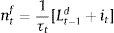
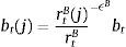
In the second version, firms receive funds from banks. In other words, the decision on how much to lend and at what price is entirely taken by the bank. The decision depends basically on three factors: their market power in the retail branch, the cost of managing bank capital in the wholesale branch, and the adjustment costs in changing the lending rate by the retail branch. The second component is moreover time-varying, which means that the capital level will fluctuate over the business cycle.5 This approach in modelling the financial sector follows Gerali, Neri, Sessa, and Signoretti (2010) who model Euro Area financial sector and corporate financing in this way.
To sum up, firms like market-based financing because it is more flexible and, conditional on positive market outlook, credit is relatively cheaper. Conversely, as in Bolton and Freixas (2006), bank credit is attractive because it is more stable and there is a lower probability of sharp reductions in supply during downturns since banks interiorise the risks from heavy market downturns (using their capital buffers). At the same time it is also more expensive because of capital adequacy-and adjustment costs.
Both mechanisms are embedded in an otherwise identical dynamic general equilibrium structure of De Grauwe and Gerba (2015).
2.1Market funding structureTo remind the reader about the corporate financing mechanism modelled in De Grauwe and Gerba (2015) and De Grauwe and Macchiarelli (2015) models, we will just briefly outline it here.
Firms borrow money from the market paying an interest rate that normally exceeds the risk-free interest rate. Hence the cost of market funds eftt is equal to the risk free rate rt plus a spread xt as:

The spread between the two rates depends on firms’ equity:
where ψ<0. This is a parameter on firm equity and represents the share of equity that cannot be used for borrowing. As the value goes down, more of firm equity can be used as collateral for borrowing.6 Following the financial accelerator approach used in Bernanke, Gertler and Gilchrist (1999), markets charge a premium xt for the perceived credit risk from providing the funds. When the value of equity rises, markets interpret this as an increase in a firm's stake in the project, which reduces firms’ incentives to invest money in unproductive projects or default. This improves its solvency and the perceived credit risk falls. The exact opposite occurs when the price of equity falls.7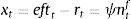
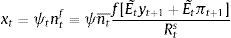
In order to have asset price variability contribute to volatility in firms’ equity, we connect firms’ market capitalization to the number of time-varying shares nt¯ multiplied by the current share price St, or:

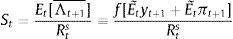
We use the standard Gordon discounted dividend model to derive share prices:
where;with Et[Λt+1¯ denoting expected future dividends net of a discount rate Rts. The rate consists of a risk-free component rt and a constant equity premium ξ. Hence asset prices are determined by the expected dividend growth. In the stable growth Gordon model, dividends grow at a constant rate. Moreover, agents assume that the 1-period ahead forecast of dividends is a fraction f of nominal GDP one period ahead.8 Since nominal GDP consists of a real and inflation component and agents have imperfect beliefs about both, they make a forecast about future (real) output- and inflation gaps. These forecasts are re-evaluated in every period. Agents are willing to switch to another forecasting rule if this performs better than the current rule (we will describe this in further detail in Section 2.4).

If agents forecast a positive output gap and/or inflation in the future, then via the Gordon model, asset prices will also increase, relaxing firms’ borrowing constraint. When all agents forecast a positive output/inflation gap (sentiment index=1), we say that agents are optimists. When the index is zero, or all agents forecast a negative output gap, agents become pessimistic. In that situation, asset prices will fall, reducing the value of firm collateral and thus their borrowing capacity. In spirit of De Grauwe and Macchiarelli (2015), we call the fluctuations in agents’ forecasts (or market sentiment) animal spirits.
Following the literature, a firm's leverage ratio is defined as loans (Ltd) over equity (nt¯St), or:

This leverage ratio is time-varying, and therefore endogenous to the business cycle. Using the assumption in De Grauwe and Macchiarelli (2015) that firms use all external funds to invest, investment and loan demand are linked by:

Combining Eqs. (6) and (7), it becomes clear that firm net worth depends on the inverse of firm leverage ratio (τt) according to:
In other words, the more a firms is leveraged, the stronger the amplification effect of asset price movements on firm borrowing capacity. An increase in the value of stock prices increases the value of collateral and reduces leverage. These two components combined lead to a more than proportional increase in its borrowing capacity. Conversely, when asset prices fall, the reduction in loans is more than proportional. That is why we should expect sharp swings in firm finances over the cycle as is typical of market-based corporate finance regimes.9
With this, we have linked the lending rate with the aggregate economy, via share prices and the collateral constraint:
We have thus closed the link between imperfect beliefs, market financing and the aggregate economy.
This mechanism is embedded into the broader behavioral model as in De Grauwe and Gerba (2015). In it, interconnectedness between stock markets, firm finances and the supply side give rise to important propagation of shocks and amplification of market sentiments.
In the next subsection, we proceed with the second version of corporate financing using banks as the (costly) loan supplier.
2.2Financial sectorWe introduce an imperfect bank-driven credit production, where banks take deposits from savers, bundle these up into multiple credit lines, and give out loans to firms at a cost determined by the intrinsic (loan) production technology. At the same time, bank manages capital in a (dynamically) rational manner in order to cushion against future shocks to its balance sheet. To facilitate the exposition, we separate the bank capital management branch (wholesale sector) from the loan management (retail sector) activity as in Gerali et al. (2010).
We can think of the banks as composed of |textbftwo retail branches and one wholesale branch. The first retail branch is responsible for giving out differentiated loans to firms and the second for raising differentiated deposits. Banks operate in a competitive environment in the wholesale sector, but behave monopolistically competitive a la Dixit-Stiglitz in the retail one. Their ability to change rates in the retail sector depends on the market power they hold in that segment (determined by the parameters ϵtB and ϵtD for the loan and deposit segment) as well as the adjustment costs.
2.2.1Wholesale branchThe balance sheet of the commercial bank can be defined as:
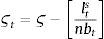
Dt are total deposits, Bt are total loans (given out to firms via the retail loan branch), and πtBntB is the real value of bank equity, where ntB is the number of stocks of banks and πtB is the price.10 The capital-to-asset ratio of a bank (or the inverse leverage) is thus: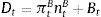

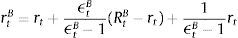
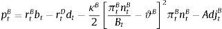
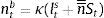
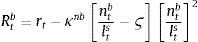
Whenever the bank deviates from the targeted capital-to-asset ratio ϑB, it pays a quadratic cost proportional to the outstanding bank capital and governed by the parameter κnB. This cost is internalized by the wholesale branch and carried over to the retail branch and end borrower via:
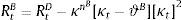
Assuming that banks have unlimited access to finance at the policy rate rt from a central bank, via arbitrage condition we can rewrite the above expression as:
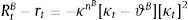
We calibrate κnB to 11.07, or the median of the estimated value in Gerali et al. (2010), and ϑB to their calibrated value of 0.09 to maintain consistency. This is a capital-to-asset ratio consistent with Basel II, and a generous leverage ratio of approximately 11%.
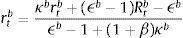
The left-hand side of Eq. (13) captures marginal benefit from increasing lending since an increase in spread equals the increase in profits. Meanwhile, the right-hand side represents the marginal cost from doing so in terms of the additional expenses arising for moving away from the optimal capital-to-loan ratio. Whenever the deviation from the target is positive (or bank has more capital than the target value, i.e. the term in brackets is positive), the right hand side will be positive, and so the spread will be smaller. Likewise, if deviation is negative, the right-hand side in Eq. (13) will be positive, and to capture the higher costs, the spread between the two rates will be larger.11 In other words, as soon as the wholesale branch incurs a capital (deviation) cost, they pass it on to the retail-lending branch (and end borrowers). By symmetry, the same applies when they hold higher capital than the required. However, since the borrowing rate cannot be lower than the policy rate, this becomes the absolute floor. Taken together, banks will optimally choose a level of loans where marginal benefits and costs are equalized.
2.2.2Loan retail branchIt obtains wholesale loans Bt at rate RtB, differentiates them and resells them to firms applying a mark-up. The mark-up is governed by a quadratic adjustment cost for changing the rate over time, and the adjustment cost in turn depends on the parameter determining the adjustment costs in loan rate setting, κB. These are proportional to aggregate return on loans. The rate charged on loans can be expressed as:
which in absence of inertias can be reduced to: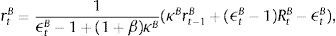
This is the external finance premium that firms are charged. The premium is proportional to the wholesale branch spread, which in turn is determined by the bank's capital position. The degree of monopolistic competition also matters since an increase in market power (a fall in ϵtB) results in a higher premium.
Following Gerali et al. (2010) and Beneš and Lees (2007), we assume that the contracts that firms use to obtain loans are a composite constant elasticity of substitution basket of slightly differentiated financial products – each supplied by a branch of a bank j – and with elasticity ϵtB, as in Dixit and Stieglitz framework.12 The elasticity is stochastic and exogenously determined. These innovations to elasticity can be seen as alterations independent from the monetary policy. Assuming symmetry amongst firms, their aggregate demand for loans at bank j can be expressed as:13
To interpret this expression, the loan that firm i gets depends on the overall volume of loans given to all firms, and on the interest rate charged on loans by bank j relative to the rate index for loans with similar characteristics.
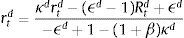
2.2.3Deposit retail branchIn an analogous way, the retail unit collect deposits from savers and passes the funds on to the wholesale branch. They remunerate these funds at rate rt. The quadratic adjustment costs for changing the deposit rate are determined by the parameter determining adjustment costs in deposit rate setting, κD, and are proportional to aggregate interest paid on deposits. Analogous to the retail-borrowing rate, the deposit rate can be described as:
which in absence of inertias, is simply a markdown over the policy rate:

The demand for deposits of saver i is symmetrically obtained to the case of loan rate determination in the previous subsection. Once again we assume that the contracts that savers use to deposit money are a composite constant elasticity of substitution basket of slightly differentiated financial products – each supplied by a branch of a bank j – and with elasticity ϵtD.14 The elasticity is stochastic and exogenously determined. Once again, these innovations to elasticity can be seen as alterations independent from the monetary policy. Assuming symmetry amongst savers, their aggregate demand for deposits at bank j can by analogy to the above case be expressed as15:
where dt are the aggregate deposits in the economy, rtD(j) is the return on deposits from bank j, and rtD is the rate index for that kind of deposits.2.2.4Bank finances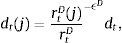
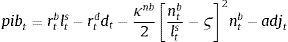
Now that we have described the dynamics of each of the branches, we are in a position to describe the finances of the aggregate bank unit. Overall bank profits (pB) are the sum of net earnings from the two retail (rtBbt−rtDdt) and one wholesale branch κB2[πtBntBBt−ϑB]2πtBntB−AdjtB:
Each period profits are accumulated in a standard fashion, and added onto existing bank equity stock according to:

Banks’ equity position has a core role in the functioning of the financial system since it (simultaneously) determines the quantity and the price of loans supplied. On one hand, it determines the external finance premium of firms. On the other, since banks pay a cost whenever they deviate from their targeted capital-to-asset ratio ϑB, banks will choose a level of loans where the marginal benefit from extending the credit portfolio equals the marginal costs for deviating from the ϑB target.
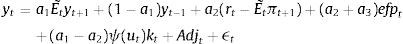
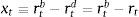
2.3Aggregate dynamicsFor the MBF model, we keep the equations as in the benchmark De Grauwe and Gerba (2015) model. In that framework, the aggregate demand equation can be expressed as:
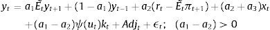
Notice that apart from the standard terms derived in De Grauwe (2011, 2012) and De Grauwe and Macchiarelli (2015), aggregate demand depends on the usable capital in the production, utkt discounted for the cost of financing (xt).
The reader will also notice that aggregate demand depends on the external finance (or risk) premium xt. This is a reduced form expression for investment, since investment is governed directly by this premium, and therefore it is the dependent variable (see De Grauwe and Macchiarelli (2015) for a derivation of this term).
In the case of BBF, we will need to make some amendments to the above expression.
First, we use expression (14) to redefine the external finance premium in (22), and get:
where a2′=ϵtB(d3+e2)1−d1, a3′=1ϵtB−1+(1+β)κB and a4′=(ϵB−1). Hence we have redefined the external finance premium xt in the aggregate demand equation. Second, banks accumulate capital and this is added to the resource constraint above. Following Gerali et al. (2010) we add the net bank equity (net of equity depreciation rate δB) to the above expression: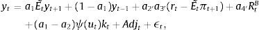
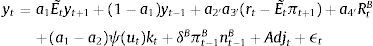
Third, we include the adjustment costs from changing the (deposit and lending) rates into the term Adjt.
As is standard, the aggregate supply (AS) equation is obtained from the price discrimination problem of retailers (monopolistically competitive):

As explained in De Grauwe and Macchiarelli (2015), b1=1 corresponds to the New-Keynesian version of AS with Calvo-pricing (Woodford, 2003).
To complete the model, we will briefly outline the learning dynamics that we make use of in this framework.
2.4Expectations formation and learningUnder rational expectations, the expectational term will equal its realized value in the next period, i.e. EtXt+1=Xt+1, denoting generically by Xt any variable in the model. However, as anticipated above, we depart from this assumption in this framework by considering bounded rationality as in De Grauwe (2011, 2012). Expectations are replaced by a convex combination of heterogeneous expectation operators Etyt+1=E˜tyt+1 and Etπt+1=E˜tπt+1. In particular, agents forecast output and inflation using two alternative forecasting rules: fundamentalist rule vs. extrapolative rule. Under the fundamentalist rule, agents are assumed to use the steady-state value of the output gap – y*, here normalized to zero against a naive forecast based on the gap's latest available observation (extrapolative rule). Equally for inflation, fundamentalist agents are assumed to base their expectations on the central bank's target – π* against the extrapolatists who naively base their forecast on a random walk approach.16We can formally express the fundamentalists in inflation and output forecasting as:
and the extrapolists in both cases as:


This particular form of adaptive expectations has previously been modelled by Pesaran (1987), and Brock and Hommes (1997, 1998), amongst others, in the literature. Setting θ=1 captures the “naive” agents (as they have a strong belief in history dependence), while a θ<1 or θ>1 represents an “adaptive” or an “extrapolative” agent (Brock & Hommes, 1998). For reasons of tractability, we set θ=1 in this model.
Note that for the sake of consistency with the DSGE model, all variables here are expressed in gaps. Focusing on their cyclical component makes the model symmetric with respect to the steady state (see Harvey & Jaeger, 1993). Therefore, as De Grauwe and Macchiarelli (2015) show, it is not necessary to include a zero lower bound constraint in the model since a negative interest rate should be understood as a negative interest rate gap. In general terms, the equilibrium forecast/target for each variable will be equal to its’ steady state value.
Next, selection of the forecasting rule depends on the (historical) performance of the various rules given by a publically available goodness-of-fit measure, the mean square forecasting error (MSFE). After the time ‘t’ realization is revealed, the two predictors are evaluated ex post using MSFE and new fractions of agent types are determined. These updated fractions are used to determine the next period (aggregate) forecasts of output-and inflation gaps, and so on. Agents’ rationality consists therefore in choosing the best-performing predictor using the updated fitness measure. There is a strong empirical motivation for inserting this type of switching mechanism amongst different forecasting rules (see De Grauwe and Macchiarelli (2015) for a brief discussion of the empirical literature, Frankel and Froot (1990) for a discussion of fundamentalist behaviour, and Cogley (2002), Cogley and Sargent (2007), Roos and Schmidt (2012) and Cornea, Hommes, and Massaro (2012) for evidence of extrapolative behaviour, in particular for inflation forecasts).
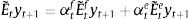
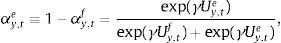
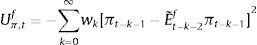
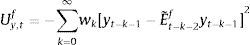
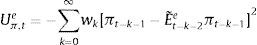
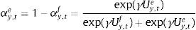
The aggregate market forecasts of output gap and inflation is obtained as a weighted average of each rule:
where αtf is the weighted average of fundamentalists, and αte that of the extrapolists. These shares are time-varying and based on the dynamic predictor selection. The mechanism allows to switch between the two forecasting rules based on MSFE/utility of the two rules, and increase (decrease) the weight of one rule over the other at each t. Assuming that the utilities of the two alternative rules have a deterministic and a random component (with a log-normal distribution as in Manski and McFadden (1981) or Anderson, De Palma, and Thisse (1992)), the two weights can be defined based on each period utility for each forecast Ui,tx, i=(y, π), x=(f, e) according to:where the utilities are defined as:and wk=(ρk(1−ρ)) (with 0<ρ<1) are geometrically declining weights adapted to include the degree of forgetfulness in the model (De Grauwe, 2012). γ is a parameter measuring the extent to which the deterministic component of utility determines actual choice. A value of 0 implies a perfectly stochastic utility. In that case, agents decide to be one type or the other simply by tossing a coin, implying a probability of each type equalizing to 0.5. On the other hand, γ=∞ implies a fully deterministic utility, and the probability of using the fundamentalist (extrapolative) rule is either 1 or 0. Another way of interpreting γ is in terms of learning from past performance: γ=0 imples zero willingness to learn, while it increases with the size of the parameter, i.e. 0<γ<∞.
As mentioned above, agents will subject the performance of rules to a fit measure and choose the one that performs best. In that sense, agents are ‘boundedly’ rational and learn from their mistakes. More importantly, this discrete choice mechanism allows to endogenize the distribution of heterogeneous agents over time with the proportion of each agent using a certain rule (parameter α). The approach is consistent with the empirical studies (Cornea et al., 2012) who show that the distribution of heterogeneous agents varies in reaction to economic volatility (Carroll, 2003; Mankiw, Reis, & Wolfers, 2004)).
2.5Calibration and model solution2.5.1CalibrationTo simplify and focus the discussion, we will only present the calibrations of the parameters that are new to this model. The remaining parameters, including the parameters specific to the MBF version of this paper, have the same values as in De Grauwe and Gerba (2015). We refer to that paper for a more detailed discussion, as well as to the parameter list in Appendix.
The parameters specific to the banking sector and the loan-deposit production are parametrized to the values in Gerali et al. (2010). This is because their model attempts to replicate the banking sector frictions present in the Euro Area, which is also our interest here. The parameters that are calibrated in their model have the same values in our BBF version. So, for instance, banks’ capital-to-asset target ratio, ς is set to 0.09 in order to reflect a low-and-stable leverage in the banking sector (which is optimal from the perspective of the macroprudential authority). Also, banks’ market power in the loan-and deposit-rate setting (ϵb and ϵd) are set to 3.12 and −1.46 in order to reflect the relative strength that banks have in assets with respect to their liabilities. Equally, banks’ cost for managing its capital is parametrized to 0.1049 as in Gerali et al. (2010) in order to induce a sufficiently high cost for banks for reducing its capital position. The intertemporal discount rate, β is standardly set to 0.9943. The initial bank capital nb¯ is set to 1, which is sufficiently low in order to allow banks to operate in the initial period.
The parameters that were estimated in Gerali et al. (2010) have been set in accordance to the results from their posterior distributions. In this way, the adjustment costs in leverage deviation, firms’ rate, and household rate (or κnb, κb, and κd) were calibrated to 11.07, 13 and 3.50 that is well within the 95% interval of the posterior. Moreover, those costs correctly reflect the varying costs that banks face in managing bank equity, producing loans and offering deposits.
All shocks, except to the capital utilization, are parametrized as white noise which means that their autoregressive component is set to 0. Likewise the standard deviations of shocks are set to 0.5 across the entire spectrum.17
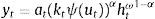
2.5.2Model solutionWe solve the model using recursive methods (see De Grauwe (2012) for further details). This allows for non-linear effects. The model has six endogenous variables, output gap, inflation, financing spread, savings, capital and interest rate. In the benchmark MBF version of the model, the first five are obtained after solving the following system:

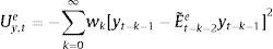
In the BBF version, the system of equations for the five variables looks instead like:
Using matrix notation, we can write this as: AZt=BE˜tZt+1+CZt−1+DXt−1+Evt. We can solve for Zt by inverting: Zt=A−1(BE˜tZt+1+CZt−1+DXt−1+Evt) and assuring A to be non-singular.
The only difference is that the equation for financing spread (line 3 in matrices A, B D and E) looks different in the two versions of the model (since the spread depends on different variables respectively).
Solution for interest rate rt is obtained by substituting yt and πt into the Taylor rule. Bank equities, credit, deposits, loan rate, deposit rate, bank profits, bank leverage, firm leverage, investment, utilization costs, labor, net worth of banks, and net worth of firms are determined by the model solutions for output gap, inflation, financing spread, savings and capital.18
Expectation terms with a tilde E˜t implies that we do not impose rational expectations. Using the system of equations above, if we substitute the law of motion consistent with heterogeneity of agents (fundamentalists and extrapolators), then we can show that the endogenous variables depend linearly on lagged endogenous variables, their equilibrium forecasts and current exogenous shocks.
Note that for the forecasts of output and inflation gap, the forward looking terms in Eqs. (22) and (25) are substituted by the discrete choice mechanism in (30). For a comparison of solutions in the ‘bounded rationality’ model and rational expectations framework, see Section 2.4 in De Grauwe and Macchiarelli (2015).
2.5.3Forcing variablesThe shock we will examine in this paper is a conventional (expansionary) monetary policy shock (ϵ)19:
where ϵ is a white noise monetary policy shock which is calibrated to 0.5 in both versions of the model. This shock is not persistent, so we set the AR(1) process to 0. Alternatively, we could have set the AR parameter to somewhere between 08 and 0.95, as is standard in the traditional DSGE literature. However, we wish to maintain consistency and facilitate comparability with previous behavioral models, and therefore choose a white noise shock.
Note in matrix E that the monetary policy shock is scaled by the leverage gap in the banking sector (ς−ςt). This gap measures how much the banking sector is away from its’ targeted (or optimal) leverage ratio. The bigger the gap, the more leveraged the banking sector, and the stronger effect a monetary policy shock will have on the system. This is in order to capture the enhanced effects that leveraging has on flows, in particular when a de-leveraging spiral is triggered.20
3Quantitative resultsWe divide our analysis in three parts. First, we will briefly discuss the impulse responses and compare the monetary transmission channels to the real economy between the two versions. Next, we will use the statistical moments (of the models and data) and ergodic distributions to analyse the role imperfect beliefs play in driving business and financial cycles and compare business cycles across the two models. The final part is a conditional exercise where our aim is to examine the effectiveness of (conventional) monetary policy in taking the economy out of a contraction and generate boom conditional on the economy already being in a bust.
Bear in kind that our ultimate interest lies in understanding how financial frictions in corporate financing influence the effectiveness of monetary policy. Therefore, except the financial friction, everything else is equal across the two models, including imperfect beliefs, learning dynamics, the remaining characteristics of the firm sector, the rest of the economy, and the type and size of shock.
3.1Impulse responses to a monetary policy shockFig. B.1 depicts the impulse responses to an expansionary monetary policy shock in the MBF version, whereas Figs. B.2 and B.3 depict the responses to the same shock in the BBF version. We have included the responses of a large number of model variables including output, investment, capital, inflation, interest rate, deposits, loans, animal spirits, bank profits (BBF), bank equity (BBF), bank leverage (BBF), and deposit rate (BBF). The numbers on the x-axis indicate number of quarters. The shock is introduced in t=100 and we observe the responses over a long period of 60 quarters (or 15 years). The figures depict the full impulse responses with the 95% confidence intervals. The blue line represents the median impulse response, and the red lines are the 95% interval.
Examining the median responses in the MBF model in Fig. B.1, a drop in policy interest rate (0.5% fall) leads to a fall in the external finance premium, which relaxes the credit that firms can access and therefore pushes up investment (0.3%). This pushes up capital accumulation (0.4%). This initial expansion is by the market perceived as a period of positive outlook, which triggers an optimistic phase (animal spirits up 0.2%). This optimism coupled with the drop in the (benchmark) interest rate results in a noticeable increase in loans to firms (1.1% and statistically significant). Roughly, that is twice the size of the initial drop in interest rate. There are three channels at play. First, the reduction in policy rate reduces the lending benchmark rate and increases liquidity on the market, pushing the external finance premium down. At the same time, the discount factor in the Gordon dividend model falls, which increases the share price and the value of collateral, and reduces further the external finance premium. On top of that, optimism (which is reflected in the positive forecast of future output and inflation gaps) pushes the share prices up, increases the value of collateral and contracts the external finance premium.21
Turning to the BBF version in Figs. B.2 and B.3, the effects from a monetary policy expansion are, on average, twice as large. Investment rises by 0.7%, capital by 0,4% and animal spirits by 0.1%. On the financial side, banks expand their lending and leverage. On the deposit side, the rate goes up by 0.5%, attracting more deposits (0.2%). This permits banks to increase loans by 0.75%. The consequence is an increase in leverage by 0.1% many periods ahead, but also a substantial increase in bank profitability, since they rise over a long period.
On the real side, output increases by 0.4% and inflation by 0.08%. Meanwhile, in the MBF version, the expansion is more moderate at 0.20% for output and 0.01% for inflation, with a lag of 1 quarter.22
The confidence intervals are also much narrower in the BBF version. Since firm leverage plays a less central role in the intermediation mechanism of the bank-based model version, market sentiments (or the uncertainty arising from imperfect beliefs on the stock market) in Eq. (9) are not translated to the model dynamics to the same extent. As a result, the variation around the median impulse response is much smaller, and the IRF distribution is tighter.
A boom in credit caused by a monetary expansion is stronger in a market-based system. The interaction between the actual drop in interest rate with positive market outlook relaxes the credit constraint more than proportionally. While the credit expansion is significant in the bank-based system, it is somewhat smaller. This is because banks need to sustain costly capital requirements and shield it against future negative outlooks. However, the impulse response estimates in the MBF version are much wider which implies that there is a non-negligible probability of the credit expansion being smaller than in the BBF version. It mainly depends on the strength of the initial animal spirit channel.
The macroeconomic effects from this expansion, on the other hand, are stronger in the bank-based version. This is because less of the market uncertainty is passed through to the real economy, which allows it to expand more. That is why investment rises by more than twofold in the BBF version. In some sense, the marginal benefit in terms of generating aggregate growth of a unit of credit is higher in a bank-based financing system.
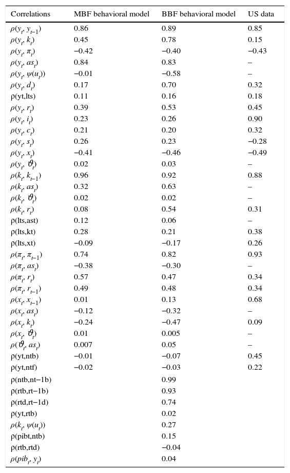
3.2Business-and financial cyclesWe simulate the model for 2000 periods (or 500 years), calculate the statistical moments for all the variables and their respective ergodic distributions and compare these to the US data. Table B.2 reports the correlations in the two models and the data. Table B.3 compare volatilities, Table B.4 skewness, and Table B.5 kurtosis between the models and the data.
Both models are capable of generating smaller cyclical fluctuations, as well as larger booms and busts. When the amplitude of the cycle is small, the financial expansion is also more limited. However, following a longer expansion, the busts are also heavier as depicted in the first two graphs of Fig. B.4. The heavy contractions extend to all variables including the standard ones such as inflation, capital, and asset prices, but also financials such as net worth and the external finance premium. But in addition, the cycles are asymmetric around the zero-line. This means that following a long expansion, the drop in most variables is deeper than the previous rise. Compared to rational expectations models, this is possible to generate because of the additional uncertainty (or friction) originating from imperfect beliefs. Following a negative shock (to, for instance, investment or technology), the usual contraction in output due to lower production–investment–purchase schedule is present. Moreover, less capital is purchased from capital goods producers, which reduces future net worth and therefore external finance possibilities. On top of that and because of imperfect forecasts regarding future productivity, a sequence of negative state variable realizations will depress the outlook of market. These negative beliefs work as accelerator of the (fundamental) shocks, and mixed with financial frictions, result in sharp drops.
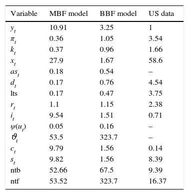
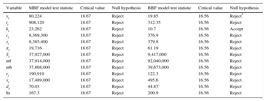
The Jacques–Bera tests in Table B.6, a visual inspection of the (ergodic) distributions in Figs. B.7 and B.8 and the moments in Tables B.3–B.5 confirm this. In both models, the null hypothesis of normality is rejected for (almost) all variables. A closer inspection of the skewness results in Table B.4 shows that most variables are skewed (left or right) and many have a high kurtosis in Table B.5.
However, both the Jacques–Bera test statistics and the moments suggest a (relatively) lower degree of non-Normality (or asymmetry and extreme values) in the BBF model. The only exceptions are asset prices, loan supply, net worth of banks, and net worth of firms. Combining this with the visual inspection in Figs. B.4–B.6, this means that even if the BBF model generates greater fluctuations in the credit variables, due to the additional level of financial frictions in banking, the pass-through to the real economy is smoother. Banks absorb some of that volatility using their capital buffers. In the MBF version, on the other hand, that volatility is directly passed on to borrowers, who include them in their intertemporal decision-making. That is why we see a higher degree of skewness and fatter tails in the aggregate economy in the MBF version.
Turning to data, note in Tables B.4 and B.5 that almost all variables in the US sample are skewed and kurtic.23 Their distributions are non-normal. Capturing these asymmetries is important in any model that tries to replicate the US economy. Evaluating the tables, for many of the variables, the BBF model does a better job. Likewise for second moments. For instance, in Table B.2 the autocorrelations of yt, kt, πt and xt are improved with respect to the market-based version. The correlations of financial market variables are also considerably improved.
3.3Monetary stimulus in recessions: when is it more effective?The final part concerns the responsiveness and effectiveness of monetary policy conditional on a recession. This is different from the overall effectiveness we studied in the impulse response analysis, as we condition the economy to be in a recession by simulating the model for 2000 periods and extract those when the economy is in a recession. During those periods, we examine by how much and how frequently the interest rate drops and the effect these drops have on the subsequent path of the other variables. Remember that the basic models include only one shock. Therefore we can clearly identify the exogenous processes that drive the underlying model dynamics in the simulations. Since 2000 periods is a long sample, we zoom in 100 of those in Figs. B.4–B.6 and study this conditional dynamics.
Earlier we mentioned that the cyclical swings in output are heavier in the MBF version. Yet from the last row of graphs in Fig. B.4 monetary policy is more accommodative in recessions in the BBF model. Both the total number of interest rate drops and the depth, on average, of each is higher. The sharpest drop of more than 5% around t=340, for instance, does not at all occur in the MBF model. On the contrary, the hikes in interest rates are instead sharper in the MBF version.
The total effect on output from these interest rate cuts is nonetheless more modest. Taking into account that output expansions are weaker in BBF (by up to 1/3 compared to MBF), the more accommodative monetary policy in this version does not equally translate into heavy booms. The reason, we believe, is the capital restrictions that banks face in downturns (since it is highly probable that their capital-to-loan ratio falls) that does not allow them to fully make use of the new liquidity to extend lending in the same proportion. Equally, the emerging positive market outlook will improve firm's capital position, but not as quickly as in the MBF version (due to more restricted credit), which in turn will moderate the self-fulfilling effects on market sentiment, and thus growth.
Yet, in the context of the Great Recession and consumption smoothing, the role of interest rate in smoothing the cycles of output has become equally (if not more) important. If the aim of the monetary policy is to smoothen the business cycle (via expected inflation), then this objective is fulfilled to a greater extent in the BBF version. The volatility of the business cycle is more than 10% less than that of the MBF version. Hence monetary policy in the BBF version is more successful in achieving economic stability.
4Discussion and concluding remarksThe effectiveness of monetary policy in reviving stagnating economies has once again become a key priority for policy makers in advanced and emerging economies during the Great Recession. The extent to which monetary easing can restore confidence on financial markets as well as reinstate economic growth has been a key priority for the Fed, ECB, Bank of England, Bank of Japan, and more recently for central banks in BRICS countries. Their success in achieving those objectives, however, is still very unclear.
We look at one aspect of this problematic in the current paper. We examine the relative effectiveness of monetary policy in a bank-based and in a market-based (corporate) financing system. Our aim is to understand whether the monetary transmission mechanism is more effective when banks or markets provide the majority of liquidity in the economy. Bank credit is preferred because it is more stable. On the other hand, the benefits from market loans are that they are flexible and more of it is available in upturns.
In the impulse response analysis, we find that a credit boom caused by a monetary expansion is stronger in a market-based system. The interaction between the actual drop in interest rate with positive market outlook relaxes the credit constraint more than proportionally. That said, the impulse response estimates in the MBF version are much wider which implies that there is a non-negligible probability of the credit expansion being smaller than in the BBF version. It mainly depends on the strength of the initial animal spirit channel.
The macroeconomic effects from this expansion, on the other hand, are stronger in the bank-based version. This is because less of the market uncertainty is passed through to the real economy, which allows it to expand more. In some sense, the marginal benefit of a unit of credit is higher in a bank-based financing system.
To conclude, we evaluate the effect of monetary expansions conditional on the economy being in a recession. While interest rate cuts are more frequent and larger in the BBF model, the total effect on output is more modest. Capital restrictions and the limited influence of market sentiment in loan supply decisions limit the full-fledged expansionary effects from interest rate cuts compared to the MBF model. Then again, if the aim of monetary policy is to reduce the volatility in the economy (for financial or consumption smoothing purposes), then a monetary policy in the BBF model accomplishes this objective in a more effective way.
Yet, in the context of the Great Recession and consumption smoothing, the role of interest rate in smoothing the cycles of output has become equally (if not more) important. If the aim of the monetary policy is to smoothen the business cycle (via expected inflation), then this objective is fulfilled to a greater extent in the BBF version. The volatility of the business cycle is more than 10% less than that of the MBF version. Hence monetary policy in the BBF version is more successful in achieving economic stability.
There are several ways in which the current work can be extended. First, the framework can be extended to an open-economy setting. Considering that global trade has increased the degree of openness of many economies, the interaction between monetary policy and the external sector is an important mechanism. This is ignored in the current paper, and therefore the sensitivity of monetary policy to external shocks is completely overlooked.
Second and possibly more interesting would be to include a mixture model of financing in our framework. Instead of studying separately a pure bank based and market-based system, a more realistic approach is to include both but with different weights depending on the economy at study. That would bring this framework closer to the one of Bolton and Freixas (2006), but again different to theirs, allow us to additionally study the important interaction between imperfect beliefs and the financial system. It would also represent a more general version of the current theoretical set-up.
Lastly, we calibrate our parameters in the model. An interesting exercise would be to estimate the parameters of the model in order to get a more accurate representation of the business cycles.
Conflict of interestsThe authors declare that they have no conflict of interest.
Aggregate demand:
Aggregate demand:
Investment

External finance premium

Consumption

Aggregate supply:
Cobb–Douglas production function
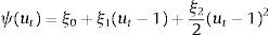
Utilization cost function
Approximated Philips curve:
Capital evolution

Cash-in-advance constraint
Labour market

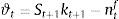
Monetary policy

Financial market:
Bank net worth
Evolution of bank leverage

Stock market price
Firm net worth

Deposits

Loan demand

Credit market equilibrium

Bank-based financing system:

Learning environment:
Inflation learning
Output learning
Learning rules:

Weights
Utilities:
ShocksMonetary policy shock:

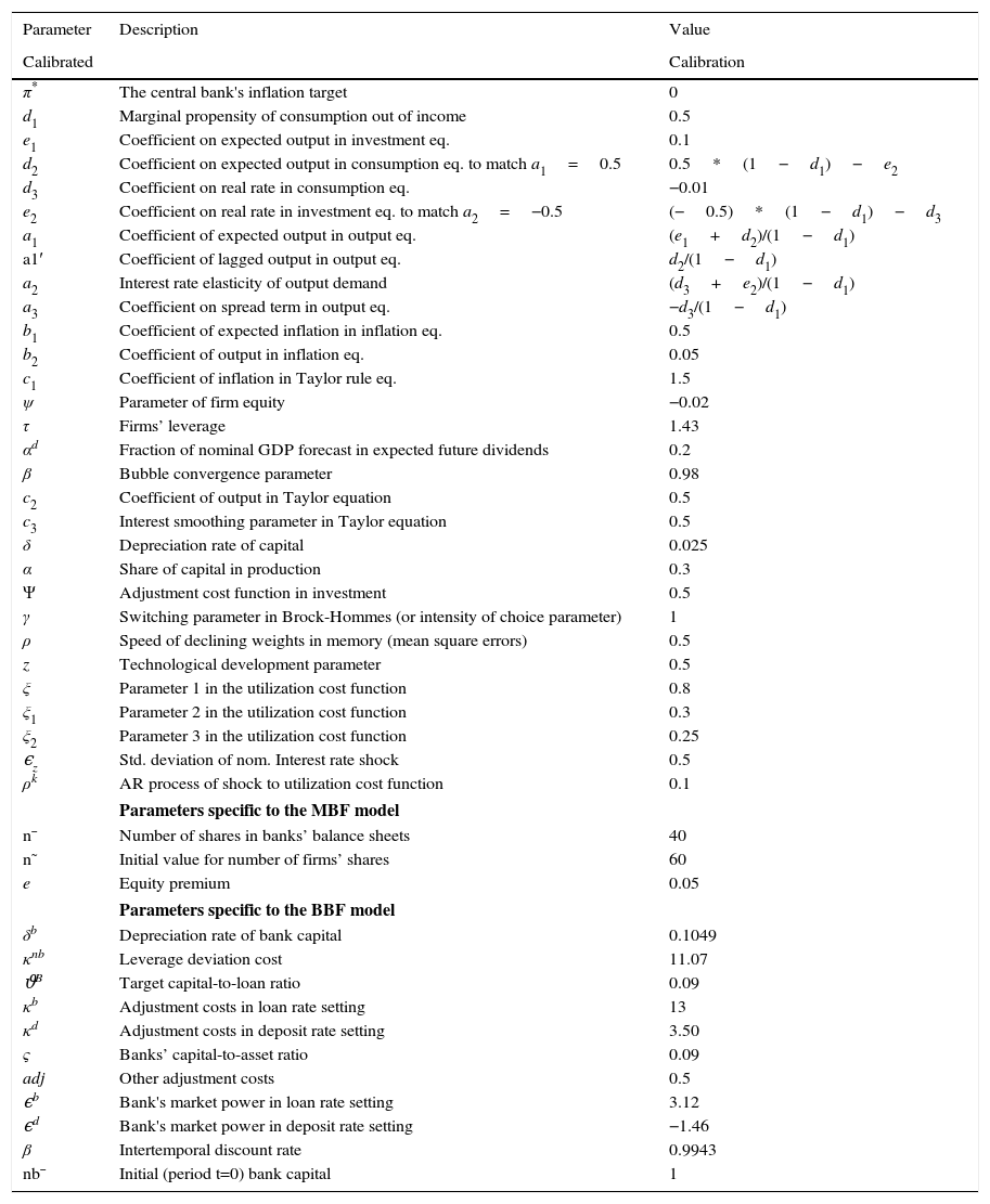
Parameters of the behavioral model and descriptions.
| Parameter | Description | Value |
|---|---|---|
| Calibrated | Calibration | |
| π* | The central bank's inflation target | 0 |
| d1 | Marginal propensity of consumption out of income | 0.5 |
| e1 | Coefficient on expected output in investment eq. | 0.1 |
| d2 | Coefficient on expected output in consumption eq. to match a1=0.5 | 0.5*(1−d1)−e2 |
| d3 | Coefficient on real rate in consumption eq. | −0.01 |
| e2 | Coefficient on real rate in investment eq. to match a2=−0.5 | (−0.5)*(1−d1)−d3 |
| a1 | Coefficient of expected output in output eq. | (e1+d2)/(1−d1) |
| a1′ | Coefficient of lagged output in output eq. | d2/(1−d1) |
| a2 | Interest rate elasticity of output demand | (d3+e2)/(1−d1) |
| a3 | Coefficient on spread term in output eq. | −d3/(1−d1) |
| b1 | Coefficient of expected inflation in inflation eq. | 0.5 |
| b2 | Coefficient of output in inflation eq. | 0.05 |
| c1 | Coefficient of inflation in Taylor rule eq. | 1.5 |
| ψ | Parameter of firm equity | −0.02 |
| τ | Firms’ leverage | 1.43 |
| αd | Fraction of nominal GDP forecast in expected future dividends | 0.2 |
| β | Bubble convergence parameter | 0.98 |
| c2 | Coefficient of output in Taylor equation | 0.5 |
| c3 | Interest smoothing parameter in Taylor equation | 0.5 |
| δ | Depreciation rate of capital | 0.025 |
| α | Share of capital in production | 0.3 |
| Ψ | Adjustment cost function in investment | 0.5 |
| γ | Switching parameter in Brock-Hommes (or intensity of choice parameter) | 1 |
| ρ | Speed of declining weights in memory (mean square errors) | 0.5 |
| z | Technological development parameter | 0.5 |
| ξ | Parameter 1 in the utilization cost function | 0.8 |
| ξ1 | Parameter 2 in the utilization cost function | 0.3 |
| ξ2 | Parameter 3 in the utilization cost function | 0.25 |
| ϵz | Std. deviation of nom. Interest rate shock | 0.5 |
| ρk | AR process of shock to utilization cost function | 0.1 |
| Parameters specific to the MBF model | ||
| n¯ | Number of shares in banks’ balance sheets | 40 |
| n˜ | Initial value for number of firms’ shares | 60 |
| e | Equity premium | 0.05 |
| Parameters specific to the BBF model | ||
| δb | Depreciation rate of bank capital | 0.1049 |
| κnb | Leverage deviation cost | 11.07 |
| ϑB | Target capital-to-loan ratio | 0.09 |
| κb | Adjustment costs in loan rate setting | 13 |
| κd | Adjustment costs in deposit rate setting | 3.50 |
| ς | Banks’ capital-to-asset ratio | 0.09 |
| adj | Other adjustment costs | 0.5 |
| ϵb | Bank's market power in loan rate setting | 3.12 |
| ϵd | Bank's market power in deposit rate setting | −1.46 |
| β | Intertemporal discount rate | 0.9943 |
| nb¯ | Initial (period t=0) bank capital | 1 |
Model correlations – comparisons.
| Correlations | MBF behavioral model | BBF behavioral model | US data |
|---|---|---|---|
| ρ(yt, yt−1) | 0.86 | 0.89 | 0.85 |
| ρ(yt, kt) | 0.45 | 0.78 | 0.15 |
| ρ(yt, πt) | −0.42 | −0.40 | −0.43 |
| ρ(yt, ast) | 0.84 | 0.83 | – |
| ρ(yt, ψ(ut)) | −0.01 | −0.58 | – |
| ρ(yt, dt) | 0.17 | 0.70 | 0.32 |
| ρ(yt,lts) | 0.11 | 0.16 | 0.18 |
| ρ(yt, rt) | 0.39 | 0.53 | 0.45 |
| ρ(yt, it) | 0.23 | 0.26 | 0.90 |
| ρ(yt, ct) | 0.21 | 0.20 | 0.32 |
| ρ(yt, st) | 0.26 | 0.23 | −0.28 |
| ρ(yt, xt) | −0.41 | −0.46 | −0.49 |
| ρ(yt, ϑt) | 0.02 | 0.03 | – |
| ρ(kt, kt−1) | 0.96 | 0.92 | 0.88 |
| ρ(kt, ast) | 0.32 | 0.63 | – |
| ρ(kt, ϑt) | 0.02 | 0.02 | – |
| ρ(kt, rt) | 0.08 | 0.54 | 0.31 |
| ρ(lts,ast) | 0.12 | 0.06 | – |
| ρ(lts,kt) | 0.28 | 0.21 | 0.38 |
| ρ(lts,xt) | −0.09 | −0.17 | 0.26 |
| ρ(πt, πt−1) | 0.74 | 0.82 | 0.93 |
| ρ(πt, ast) | −0.38 | −0.30 | – |
| ρ(πt, rt) | 0.57 | 0.47 | 0.34 |
| ρ(πt, rt−1) | 0.49 | 0.48 | 0.34 |
| ρ(xt, xt−1) | 0.01 | 0.13 | 0.68 |
| ρ(xt, ast) | −0.12 | −0.32 | – |
| ρ(xt, kt) | −0.24 | −0.47 | 0.09 |
| ρ(xt, ϑt) | 0.01 | 0.005 | – |
| ρ(ϑt, ast) | 0.007 | 0.05 | – |
| ρ(yt,ntb) | −0.01 | −0.07 | 0.45 |
| ρ(yt,ntf) | −0.02 | −0.03 | 0.22 |
| ρ(ntb,nt−1b) | 0.99 | ||
| ρ(rtb,rt−1b) | 0.93 | ||
| ρ(rtd,rt−1d) | 0.74 | ||
| ρ(yt,rtb) | 0.02 | ||
| ρ(kt, ψ(ut)) | 0.27 | ||
| ρ(pibt,ntb) | 0.15 | ||
| ρ(rtb,rtd) | −0.04 | ||
| ρ(pibt, yt) | 0.04 | ||
Note: GDP deflator was used as the inflation indicator, 3-month T-bill for the risk-free interest rate, the deposit rate as the savings indicator and the Corporate lending risk spread (Moody's 30-year BAA-AAA corporate bond rate) as the counterpart for the firm borrowing spread in the models. Variables that are left blank do not have a direct counterpart in the data (deep variables).
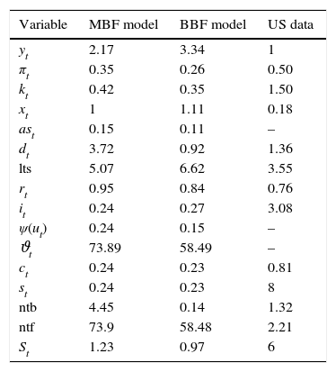
Second moments – comparison.
| Variable | MBF model | BBF model | US data |
|---|---|---|---|
| yt | 2.17 | 3.34 | 1 |
| πt | 0.35 | 0.26 | 0.50 |
| kt | 0.42 | 0.35 | 1.50 |
| xt | 1 | 1.11 | 0.18 |
| ast | 0.15 | 0.11 | – |
| dt | 3.72 | 0.92 | 1.36 |
| lts | 5.07 | 6.62 | 3.55 |
| rt | 0.95 | 0.84 | 0.76 |
| it | 0.24 | 0.27 | 3.08 |
| ψ(ut) | 0.24 | 0.15 | – |
| ϑt | 73.89 | 58.49 | – |
| ct | 0.24 | 0.23 | 0.81 |
| st | 0.24 | 0.23 | 8 |
| ntb | 4.45 | 0.14 | 1.32 |
| ntf | 73.9 | 58.48 | 2.21 |
| St | 1.23 | 0.97 | 6 |
Note: The moments are calculated taking output as the denominator. Following a standard approach in the DSGE literature, this is in order to examine the moments with respect to the general business cycle.
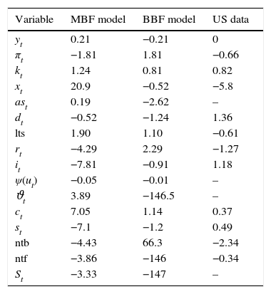
Third moments – comparison.
| Variable | MBF model | BBF model | US data |
|---|---|---|---|
| yt | 0.21 | −0.21 | 0 |
| πt | −1.81 | 1.81 | −0.66 |
| kt | 1.24 | 0.81 | 0.82 |
| xt | 20.9 | −0.52 | −5.8 |
| ast | 0.19 | −2.62 | – |
| dt | −0.52 | −1.24 | 1.36 |
| lts | 1.90 | 1.10 | −0.61 |
| rt | −4.29 | 2.29 | −1.27 |
| it | −7.81 | −0.91 | 1.18 |
| ψ(ut) | −0.05 | −0.01 | – |
| ϑt | 3.89 | −146.5 | – |
| ct | 7.05 | 1.14 | 0.37 |
| st | −7.1 | −1.2 | 0.49 |
| ntb | −4.43 | 66.3 | −2.34 |
| ntf | −3.86 | −146 | −0.34 |
| St | −3.33 | −147 | – |
Note: The moments are calculated taking output as the denominator. Following a standard approach in the DSGE literature, this is in order to examine the moments with respect to the general business cycle.
Fourth moments – comparison.
| Variable | MBF model | BBF model | US data |
|---|---|---|---|
| yt | 10.91 | 3.25 | 1 |
| πt | 0.36 | 1.05 | 3.54 |
| kt | 0.37 | 0.96 | 1.66 |
| xt | 27.9 | 1.67 | 58.6 |
| ast | 0.18 | 0.54 | – |
| dt | 0.17 | 0.76 | 4.54 |
| lts | 0.17 | 0.47 | 3.75 |
| rt | 1.1 | 1.15 | 2.38 |
| it | 9.54 | 1.51 | 0.71 |
| ψ(ut) | 0.05 | 0.16 | – |
| ϑt | 53.5 | 323.7 | – |
| ct | 9.79 | 1.56 | 0.14 |
| st | 9.82 | 1.56 | 8.39 |
| ntb | 52.66 | 67.5 | 9.39 |
| ntf | 53.52 | 323.7 | 16.37 |
Note: The moments are calculated taking real GDP as the denominator. These are calculated using the full sample of US data stretching from 1953:I to 2014:IV. During this period, the US economy experienced 10 cycles (using NBER business cycle dates), and the average GDP increase per quarter during expansions was 1.05% while it was −0.036% during recessions. Data were de-trended using a standard two-sided HP filter. The variables that are left blank do not have a direct counterpart in the data sample.
Jacques–Bera normality test results.
| Variable | MBF model test statistic | Critical value | Null hypothesis | BBF model test statistic | Critical value | Null hypothesis |
|---|---|---|---|---|---|---|
| yt | 80,224 | 18.67 | Reject | 19.85 | 16.56 | Reject* |
| it | 908,120 | 18.67 | Reject | 312.35 | 16.56 | Reject |
| kt | 23,262 | 18.67 | Reject | 10.7 | 16.56 | Accept |
| ct | 8,369,300 | 18.67 | Reject | 376.9 | 16.56 | Reject |
| st | 8,385,400 | 18.67 | Reject | 379.8 | 16.56 | Reject |
| πt | 19,716 | 18.67 | Reject | 61.19 | 16.56 | Reject |
| St | 37,927,000 | 18.67 | Reject | 9,417,000 | 16.56 | Reject |
| ntf | 37,914,000 | 18.67 | Reject | 92,040,000 | 16.56 | Reject |
| ntb | 37,868,000 | 18.67 | Reject | 39,673,000 | 16.56 | Reject |
| rt | 190,910 | 18.67 | Reject | 122.3 | 16.56 | Reject |
| xt | 17,489,000 | 18.67 | Reject | 495.6 | 16.56 | Reject |
| dt | 70.03 | 18.67 | Reject | 44.87 | 16.56 | Reject |
| lts | 167.3 | 18.67 | Reject | 200.9 | 16.56 | Reject |
Note: The results from the Jacques–Bera normality test are reported here. Second to fourth column represent the results for the MBF model, and fifth to seventh for the BBF version. Numbers above the critical values imply that the null hypothesis that a particular variable has a normal distribution is rejected. The critical values are calculated based on a Monte-Carlo simulation. The statistics for most variables (except for asset prices St, net worth of firms ntf, net worth of banks ntb, and loan supply lts) are significantly lower in the BBF version compared to the MBF one. This confirms the graphical inspection that the ergodic distributions of BBF model variables is much closer to Gaussian compared to the MBF variables.


 vs BBF (right) models. The model is simulated for 500 years but to facilitate the visibility of the process, we zoom in 25 of those years.")
 vs BBF (right) models 2.")
 vs BBF (right) models 3.")
 vs BBF (right). The histograms are calculated using a simulated sample of 500 years. The histograms can also be interpreted as ergodic distributions. See De Grauwe and Gerba (2015) for an analysis of the sine in frequency domain.")
Histograms of output gap, inflation and animal spirits in MBF (left) vs BBF (right). The histograms are calculated using a simulated sample of 500 years. The histograms can also be interpreted as ergodic distributions. See De Grauwe and Gerba (2015) for an analysis of the sine in frequency domain.
 vs BBF (right) 2. The histograms are calculated using a simulated sample of 500 years. The histograms can also be interpreted as ergodic distributions.")
 on the vertical axes means that the entire population uses the extrapolative (fundamentalist) rule to forecast the variable. This can be interpreted as the degree of regime switches that occur during the agents’ learning process. The third graph depicts the level of ‘optimism’ and ‘pesimism’ on the stock markets, where 1 is a pure bullish (or optimistic) market, 0 is a pure bearish (or pessimistic), and 0.5 is neither (or no sentiment-driven dynamics). Graphs on the left are those of the MBF version and those on the right are of the BBF.")
The first two graphs depict the fraction of the total population of agents that use the extrapolative rule to forecast output- and inflation gap. 1 (or 0) on the vertical axes means that the entire population uses the extrapolative (fundamentalist) rule to forecast the variable. This can be interpreted as the degree of regime switches that occur during the agents’ learning process. The third graph depicts the level of ‘optimism’ and ‘pesimism’ on the stock markets, where 1 is a pure bullish (or optimistic) market, 0 is a pure bearish (or pessimistic), and 0.5 is neither (or no sentiment-driven dynamics). Graphs on the left are those of the MBF version and those on the right are of the BBF.
Kashyap, Stein, and Wilcox (1996) extend their initial study above and show that even when the level effect is accounted for so that large (small) firms increase (reduce) all types of financing during a monetary tightening, there is a considerable substitution away from bank loans towards commercial paper. Calomiris, Himmelberg, and Wachtel, 1995, June and Ludvigson (1998) reach the same conclusion.
We would first of all like to thank two anonymous referees for their extremely useful and constructive comments. We would also like to express our gratitude to Vincenzo Quadrini for assisting us in making the paper more concise and sharpen the key message. Likewise, we extend our sincerest thanks to participants at the ESPE Conference organised by Banco de la Republica, participants at the external speaker programme at EF of University of Ljubljana, and the 2016 WEHIA Conference for their useful insights and comments. Lastly, we greatfully acknowledge funding from the European Commission and the FinMap project. Disclaimer: The views expressed in this paper are solely ours and should not be interpreted as reflecting the views of Bank of Spain, the Eurosystem, nor those of European Commission.
They do find some, but limited evidence of a loan supply channel in their data.
There is a large literature incorporating various financing regimes of firms in their general equilibrium modelling. However, models that specifically look at the various (and asymmetric) effects of monetary policy on firm financing under different regimes have been fewer.
The focus of their paper is, on the other hand, on imperfect substitutability between external finances and whether monetary policy can influence the preferences for one over the other.
We interiorise the entire credit granting decision to the bank in order to carefully study the interaction between bank capital, credit production and monetary policy. The emphasis is thus on the capital cost channel of banking. We do this in order to make a clear distinction to the market valuation (or sentiment) channel in the other version. While there is a collateral constraint included in the banking version, it is of second order importance. Hence firm leverage plays a role for the lending rate to the extent that the higher the leverage, the lower a firm's net worth becomes, which reduces the firm's possibility to negotiate a favourable loan with the retail branch of the bank.
You can think of it as the financial innovation parameter. A more dynamic financial innovation environment (or lower ψ) allows markets to extract a higher rate of firm equity in case the firm defaults and allows firms to use more of it to borrow.
In De Grauwe and Gerba (2015) and De Grauwe and Macchiarelli (2015) banks provide loans to firms. However these banks operate under zero profit and act as shadow lenders. In reality what determines whether and what quantity firms can borrow is the value of their internal funds, or equity. The price of equity is determined by the stock market. Hence, the stock market determines if and how much firms can borrow. Therefore banks balance sheet is not necessary in this lending mechanism and can be directly reduced to market-type of lending.
Just as in De Grauwe and Gerba (2015), dividends are assumed to be constant thereafter.
Note that asset prices affect aggregate demand indirectly, via credit spread dynamics, and do not have direct wealth effects as in De Grauwe (2012) or De Grauwe and Macchiarelli (2015).
The price of stocks is exogenously determined and normalized for the sake of simplicity.
Moreover, banks have an incentive to increase their lending in order to increase their profits (as they work under positive profit condition). This adds an additional (albeit softer) constraint that banks will not have more capital than the required target value. If anything, they will try to go beyond it and thus incur a cost.
The loan elasticity ϵtB is assumed to be above 1.
In Gerali et al. (2010) this expression is derived after minimizing over all firms Bt(i, j) the total repayment due to the continuum of banks j, ∫01rtB(j)bt(i,j)dj, subject to [∫01bt(i,j)(ϵtB−1)/(ϵtB)dj]ϵtB/(ϵtB−1)≥bt(i). (ϵtB−1)/(ϵtB) is the marku-p that banks apply on loans. Here we just take the derived first-order-condition and aggregate amongst firms. The micro-foundations are, however, straight forward.
The deposit elasticity ϵtD is assumed to be below −1.
In Gerali et al. (2010) this expression is derived after minimizing over all savers Dt(i, j) the total repayment due to the continuum of banks j, ∫01rtD(j)dt(i,j)dj, subject to [∫01dt(i,j)(ϵtD−1)/(ϵtD)dj]ϵtD/(ϵtD−1)≤dt(i). (ϵtD−1)/(ϵtD) is the mark-up that banks apply on deposits. Here we just take the derived first-order-condition and aggregate amongst savers. The micro-foundations are, however, direct.
The latest available observation is the best forecast of the future.
The AR-component of the shock to capital utilization cost is set conservatively to 0.1, just enough to generate some persistence in the capital cost structure.
However, external financing spread, capital, and savings do not need to be forecasted as these do not affect the dynamics of the model (i.e. there is no structure of higher order beliefs as law of iterated expectations does not hold in the behavioral model). See Section 3.1 in De Grauwe and Macchiarelli (2015) for comparison of solutions under rational expectations and bounded rationality (“heuristics”).
In an extension, we also introduce other three shocks (technology, aggregate demand and capital utilization cost shocks) but here prefer to focus on the monetary transmission channel only. For the analysis of the other shocks, please refer to De Grauwe and Gerba (2015).
Before we begin with the analysis, bear in mind that the behavioral model does not have one steady state that is time invariant for the same calibration (as is standard for the DSGE method). Therefore, following a white noise shock, the model will not necessarily return to a previous steady state. If not the same steady state, it can either reach a new steady state, or have a prolonged response to the initial shock. In other words, there is a possibility for the temporary shock to have permanent effects in the model (via the animal spirits channel). That is why we draw a full distribution of impulse responses to capture the entire spectrum of responses.
However, this optimism is very brief as the monetary authority raises the interest rate (0.1%) to combat the rising inflation. The market perceives this as the end of the expansionary phase, resulting in a reversal of the sentiment to pessimism (animal spirits fall by 0.05%). The consequence is a turn in the response of macroeconomic and financial aggregates, leading to return of these variables to the steady state.