On cocaine consumption: Some lessons from Spain

Abstract

In this paper, we examine the socioeconomic factors that determine cocaine consumption in adults aged over 18 years in Spain. For data from household alcohol and drug surveys for the period 2007–2012 (EDADES 2007, 2009, 2011), we used, first, a decision tree to identify the main predictors of cocaine use and high-risk profiles of cocaine consumers and, next, a multinomial logistic regression model to explain cocaine consumption in terms of sex, age, marital status, employment status, education level, income, household size and perceived health status. The results indicate that the main predictors of cocaine use are marital status, sex, employment status, age, education level and household size. The main cocaine user propensity profile is a young single man with a low level of education and unemployed, who should, therefore, be the main target of campaigns for preventing illicit drug use.

Resumen

Este trabajo analiza los factores socioeconómicos que determinan el consumo de cocaína en adultos españoles de más de 18 años. Con los datos de las encuestas domiciliarias de alcohol y drogas para el período 2007-2012 (EDADES 2007, 2009, 2011), planteamos un modelo de árboles de decisión para identificar los principales predictores del consumo de cocaína, así como los grupos de perfiles con mayor riesgo de consumo. Al mismo tiempo, construimos un modelo de regresión logística multinomial para explicar el consumo de cocaína y sus diferentes grados de una persona adulta en función del sexo, la edad, el estado civil, la situación laboral, el nivel educativo, los ingresos, el tamaño del hogar en el que vive y la percepción que tiene de su estado de salud. Los resultados muestran que los principales predictores del consumo de cocaína en adultos en España son el estado civil, el sexo, la situación laboral, la edad, el nivel educativo y el tamaño del hogar. El perfil de adultos con mayor propensión al consumo de cocaína es el de varones jóvenes con un bajo nivel de educación, que viven solos y están desempleados. Esta debería ser, pues, la población en la que centrar las campañas de prevención del consumo de drogas ilícitas.

1

Introduction

It is estimated that between 3.6% and 6.9% of the world's adult population aged over 15 years (167 m to 315 m people) consumed illicit drugs in 2011 (UNODC, 2013). Illicit drug use annually results in about 200,000 deaths worldwide and causes distress and suffering in many more millions. Illicit drug use also undermines economic and social development, promotes crime, instability and insecurity and spreads diseases such as HIV (UNODC, 2012).

Cannabis and cocaine are the two most frequently consumed drugs in the world, although cocaine has the greatest number of addicts; data from a 2010 US household survey on drug use and health (UNODC, 2012) revealed that whereas 10% of cannabis users were addicts, in the case of cocaine, this figure was 15%. Western and Central Europe and North America are the main cocaine markets, both in terms of number of users and prevalence of use, accounting for over 50% of the world consumption in 2011, with rates of use in the previous 12 months of 1.5% and 1.2%, respectively (UNODC, 2013). At least 85 million adults in Western and Central Europe (a quarter of the adult population) have used illegal drugs at some point in their lives (EMCDDA, 2013).

Cocaine consumption trends vary between countries. While US cocaine consumption fell by 40% over the period 2006–2011 (UNODC, 2013), in countries as Spain consumption prevalence in the population aged 15–64 years has increased steadily since 2001, standing at around 3% in the period 2005–2008 and decreasing slightly thereafter to stand at 2.3% in 2011 (EDADES, 2001, 2003, 2005, 2007, 2009, 2011). Spain, in fact, consistently has the highest prevalence of cocaine use worldwide.

Cocaine use represents a major health and socioeconomic problem in Spain. Analysing causes can shed light on the population segments more prone to using drugs and help to design suitable targeted prevention strategies.¹ Leading questions include: Why is adult cocaine use in Spain among the highest in the world? What are the socioeconomic circumstances that place an adult in Spain at higher risk of becoming a cocaine user than adults in other similar countries?

Studies on the socioeconomic determinants of cocaine use in Spain are relatively recent. To illustrate, Royo-Bordonada et al. (1997) suggested that a lack of employment opportunities has a statistically significant positive effect on cocaine use. On the other hand, and using data collected between 2004 and 2006, Pulido et al. (2009) described the sociodemographic characteristics of young cocaine users from the three biggest cities in Spain (Madrid, Barcelona and Seville), confirming a lower education level and higher unemployment rates in crack users and the existence of two different subpopulations among consumers of cocaine according to whether or not they consume freebase cocaine.² Likewise, (Galicia et al., 2014) described a user profile and confirmed cocaine to be the illegal drug that generated most consultations in hospital emergency departments in Spain.

Cocaine consumption is very costly for society as noted for a number of studies. For the region of Galicia (NW Spain) by Oliva and Rivera (2006) estimated—for data for addicts attending drug dependency centres in the Galician healthcare network—a cost associated with illegal drug use of around 130 million euros in 2003. Of which 33% were direct healthcare costs, including those generated by HIV/AIDS care, and the remaining 67% were indirect costs associated with productivity losses due to disability, absenteeism and premature mortality. Likewise, a study of 2007–2009 data corresponding to adults in Valencia in eastern Spain confirmed that the profile for cocaine relapse includes individuals from broken homes, with a low educational level and unemployed or in poorly paid employment (Sánchez-Hervás et al., 2012).

In this paper, we tried to find an explanation for the high level of cocaine consumption in Spain with respect to other countries. In particular, bearing in mind that the average age of onset in Spain is 21 years for powder cocaine and 22.4 years for freebase cocaine (EDADES, 2011), our first objective was to identify and classify the profiles and characteristics of adults in Spain at greatest risk by identifying the factors that motivate them to use cocaine. The second objective was to determine the weight of different factors in the decision to consume. Achieving both goals we expected to be able to predict cocaine use in Spain by classifying and applying rules and by evaluating influential factors.

The data used to carry out the current study were obtained from the Spanish Household Alcohol and Drugs Survey (EDADES) of individuals aged 15–64 years conducted in 2007, 2009 and 2011. The surveys collected data between November 2007 and March 2008, between November 2009 and March 2010, and between November 2011 and April 2012.

To identify predictors of cocaine use (consumption patterns) and population groups at risk, we used a decision tree model that graphically represented relationships between variables. This enabled us to describe cocaine user profiles and to identify complex structural relationships and so, in turn, identify combinations of predictors. Combinations of socioeconomic variables, which, in isolation, might not represent determining factors, identified propensities for cocaine use. As for the second objective, we used a multinomial regression model to isolate the socioeconomic factors that had the greatest bearing on the prevalence of cocaine use in Spanish adults.

Our results indicate that the most important predictors are marital status, sex, employment status, age, education level and household size. Specifically, profiles of Spanish adult population most likely to consume cocaine are single inactive men aged 25–50 years with an income in the third decile and single men under 36 years old, with only a basic education level, and employed or unemployed.

The regression model calculated weights for the factors selected in the decision trees as the best predictors of cocaine use. Our results indicated that living with a partner increases the probability of being a non-user by 1.8, being female reduces prevalence of use by 1.8, whereas each additional year increases the probability of being a non-user by 0.08. The model also points to the statistically significant influence of other variables such as household size, health perception, employment status, education level and income level.

The results allow us to conclude that cocaine prevention and education policies in Spain should be reoriented to especially target single middle-aged inactive men with a low level of education, bearing in mind that this target is particularly difficult to reach because these individuals have no fixed points of contact or support in universities or companies.

The rest of the paper is organized as follows. In Section 2 we describe the decision tree and multinomial regression models used to explain cocaine use in socioeconomic terms; we also describe how data was collected and descriptively analyzed. In Section 3 the main results are presented and, finally, in Section 4 we discuss those most relevant from the point of view of the adoption of targeted policies aimed at preventing or reducing cocaine use in individuals at risk.

2

Methodology and data

To measure consumption of cocaine we counted the number of days cocaine was used in the 12 months before the interview. This resulted in four cocaine user categories, namely, non-users, occasional, regular and frequent users. A non-user (Y₀) has never consumed cocaine or has not done so in the last 12 months, whereas an occasional, regular and frequent user has consumed cocaine on 1–9 days (Y₁), 10–29 days (Y₂), and more than 30 days (Y₃) in the past 12 months, respectively. We studied user profiles and the influence of socioeconomic variables using decision trees and logistic regression.

2.1

Decision trees

To analyze the predictive value of variables that may influence cocaine use we used a recursive partitioning model of decision tree. This nonparametric technique, which treats all variables as categorical variables, takes into account interactions between the data. We identify the most important predictive variables from the set of explanatory variables and classify individuals into risk groups. Because cocaine use is a categorical variable we used decision trees to graphically represent a set of decision rules. Starting from a root node (which includes all the individuals), the tree branches out into different child nodes contain subgroups of individuals. AID (Automatic Interaction Detection) software (Sonquist et al., 1971) was one of the first methods developed for fitting data based on classification tree models. It uses a recursive algorithm that successively partitions the original data in other smaller and more homogeneous subgroups using binary partition sequences.

CHAID (Chi-squared Automatic Interaction Detection) (Kass, 1980), a recursive non-binary classification algorithm, applies the chi-square test as a criterion for partitioning and uses the threshold above statistical significance as the stopping rule. In the application of this algorithm to the cocaine consumption variable (with four categories), the subproblem is repeated of reducing a given contingency table of size c×4 (where c is the number of categories of a particular predictor) to the most significant table j×4 resulting from combining prediction categories in every possible way (Kass, 1980). Formally, we calculate the statistic Tj(i) as the standard χ2 statistic for the ith method of forming the table j×4 (j = 2, 3, …, c, with the range of i depending on the type of predictor). Thus, if Tj(*)=maxi{Tj(i)} is the χ2 statistic for the best j×4 table, we choose the most significant Tj(*), i.e., that one with the lowest significance rate.

2.2

Multinomial logistic regression

The probability Y of cocaine consumption is related to a set of factors reflected in a vector X like X = (x₁, …, x_L). Since cocaine use is a discrete variable with four possible values, Y={Y0, Y1, Y2, Y3}, we choose a logistical probability function F so that the cumulative distribution function of the model results as

where (exp(X′·βj))/(1+∑k=13exp(X′·βk)) is the symmetrical logistical cumulative distribution function, X′ is a specific observation of the vector X of factors that determine the probability of an individual being a cocaine user and βj is the set of parameters reflecting the impact of changes in X on cocaine use. In particular, β0, β1, β2 and β3 measure the impact of independent variables on non-consumption, occasional consumption, regular consumption and frequent consumption, respectively.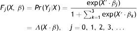

Denoting the cumulative distribution function as Λ(X·βj), we can analyze the decomposition of cocaine use depending on the covariables and using marginal effects as

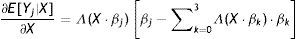
The estimated parameters of the model are obtained using the maximum likelihood method, which determines the estimate that maximizes the probability of non-consumption and of occasional, regular, and frequent consumption of cocaine, given the vector of explanatory variables. Finally, statistical significance is tested using the likelihood ratio test that follows a chi-square distribution, whereas goodness-of-fit is tested using the likelihood ratio index.

As a measure of an individual's economic circumstances we used the net monthly income of their household. In the EDADES surveys, household income is recorded as a categorical variable with eight possible responses referring to income intervals. However, since we needed a continuous measure of income, we applied an interval regression model of information provided by the respondent regarding overall household data. We thus could estimate the numerical income value from the boundaries of the intervals where the quantities are located. We took into account sex, age, educational level (no education, primary, secondary, and university), employment status (employed, unemployed, and inactive) and region of residence. Using records for 44,075 individuals from the 2007, 2009 and 2011 surveys, we generated predictions for the individual net monthly income variable.

To examine the determinants of cocaine consumption and user profiles, we first used a decision tree model and then a multinomial logit regression model with four types of explanatory variables, namely, individual characteristics, household characteristics, employment characteristics, and socioeconomic characteristics. The variables used in the regression model were as follows: sex (female omitted), age, marital status (single, partnered), household size, health perception (good, fair, and poor), educational level (no education (omitted to avoid collinearity), primary, secondary, and university), net monthly household income, and employment status.

For the polytomous cocaine use variable, we jointly considered powder cocaine and freebase cocaine use, categorized in terms of four possible values, namely, non-consumption, occasional, regular and frequent consumption. An occasional, regular, and frequent user has consumed cocaine on 1–9 days (Y₁), 10–29 days (Y₂), and more than 30 days (Y₃) in the past 12 months, respectively.

2.3

Data

Our data—for individuals aged 15–64 years and for the period 2007–2012—were taken from the EDADES household surveys for 2007, 2009 and 2011 (Galicia et al., 2014; Oliva and Rivera, 2006; Sánchez-Hervás et al., 2012) conducted by the Spanish Ministry of Health, Social Services and Equality, the Institute of Health Information (IIS), and the National Statistics Institute (INE). EDADES surveys are two-yearly surveys administered to a representative national sample stratified according to a multistage sampling procedure. The surveys collect data on alcohol and drug use and also compile information on socioeconomic, sociodemographic and geographic characteristics, and on overall health and occupation.

Our final sample was obtained as follows. We started with 65,952 individuals (23,715 from EDADES 2007 plus 20,109 from EDADES 2009 plus 22,128 from EDADES 2011). We first excluded incomplete records and records for children aged under 18, which resulted in 44,075 individuals, and we then excluded records that did not mention cocaine, which resulted in 43,984 individuals (18,416 from EDADES 2007 plus 11,530 from EDADES 2009 plus 14,038 from EDADES 2011).³ We can assume that the samples were independent since the probability that individuals were surveyed in both 2007 and 2009 was 0.0006 and the probability that individuals were surveyed in 2007, 2009 and 2011 was 0.00097.

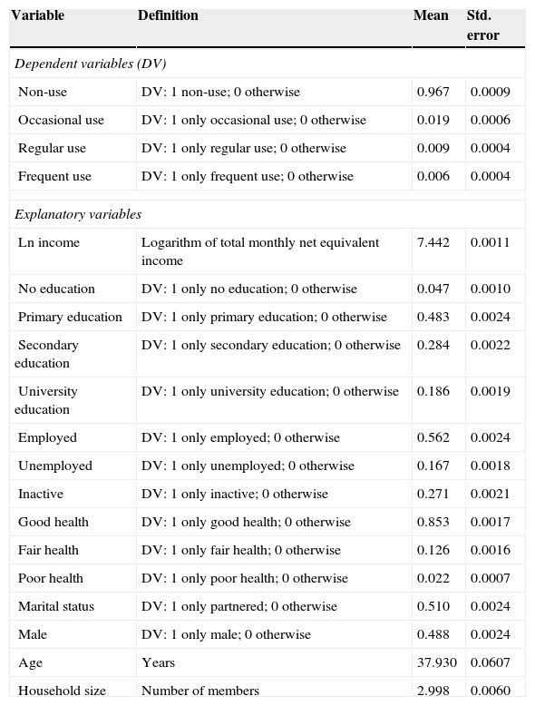
3

Results

3.1

Descriptive statistics

Table 1 below summarizes descriptive statistics referring to the prevalence of cocaine use in Spain. In addition, Fig. 1 shows frequency of cocaine use for the 43,984 individuals in our sample, calculated in terms of the number of days cocaine was used in the previous 12 months.

Table 1.

Descriptive statistics (EDADES, 2007, 2009, 2011) (N = 43,984).

Variable	Definition	Mean	Std. error
Dependent variables (DV)
Non-use	DV: 1 non-use; 0 otherwise	0.967	0.0009
Occasional use	DV: 1 only occasional use; 0 otherwise	0.019	0.0006
Regular use	DV: 1 only regular use; 0 otherwise	0.009	0.0004
Frequent use	DV: 1 only frequent use; 0 otherwise	0.006	0.0004
Explanatory variables
Ln income	Logarithm of total monthly net equivalent income	7.442	0.0011
No education	DV: 1 only no education; 0 otherwise	0.047	0.0010
Primary education	DV: 1 only primary education; 0 otherwise	0.483	0.0024
Secondary education	DV: 1 only secondary education; 0 otherwise	0.284	0.0022
University education	DV: 1 only university education; 0 otherwise	0.186	0.0019
Employed	DV: 1 only employed; 0 otherwise	0.562	0.0024
Unemployed	DV: 1 only unemployed; 0 otherwise	0.167	0.0018
Inactive	DV: 1 only inactive; 0 otherwise	0.271	0.0021
Good health	DV: 1 only good health; 0 otherwise	0.853	0.0017
Fair health	DV: 1 only fair health; 0 otherwise	0.126	0.0016
Poor health	DV: 1 only poor health; 0 otherwise	0.022	0.0007
Marital status	DV: 1 only partnered; 0 otherwise	0.510	0.0024
Male	DV: 1 only male; 0 otherwise	0.488	0.0024
Age	Years	37.930	0.0607
Household size	Number of members	2.998	0.0060

Note: Omitted categories: females, basic education, good health.

Source: (EDADES, 2007, 2009, 2011) (INE).

Figure 1.

Cocaine use frequency distribution.

Of the population aged over 18 years living in Spain, 3.3% of individuals are occasional, regular or frequent cocaine users.⁴ Just under half of these (1.4%) use cocaine regularly or frequently (at least once a month). Prevalence rates are 96.7% for non-use and 1.9%, 0.9%, and 0.6% for occasional, regular, and frequent cocaine use, respectively.

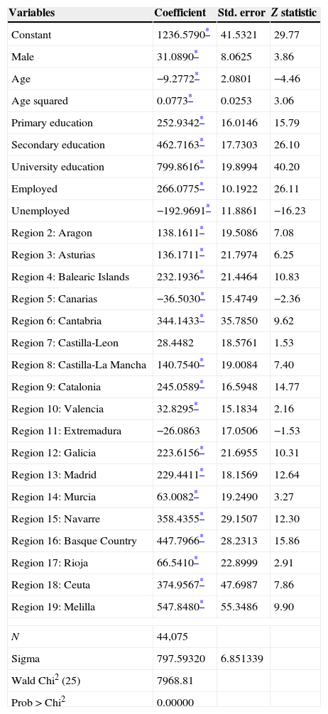
To analyze the socioeconomic circumstances, we first estimated the continuous variable of monthly net household income by applying an interval-regression model to income intervals as described in EDADES, 2007, 2009 and 2011 (the dependent variable) and age, age squared, sex, education level, employment status, and region of residence (explanatory variables). The limit values of the household income intervals were reflected in the survey. Table 2 below shows the regression estimates for household income intervals for 44,075 individuals.

Table 2.

Interval-regression model coefficients for income estimation purposes.

Variables	Coefficient	Std. error	Z statistic
Constant	1236.5790^*	41.5321	29.77
Male	31.0890^*	8.0625	3.86
Age	−9.2772^*	2.0801	−4.46
Age squared	0.0773^*	0.0253	3.06
Primary education	252.9342^*	16.0146	15.79
Secondary education	462.7163^*	17.7303	26.10
University education	799.8616^*	19.8994	40.20
Employed	266.0775^*	10.1922	26.11
Unemployed	−192.9691^*	11.8861	−16.23
Region 2: Aragon	138.1611^*	19.5086	7.08
Region 3: Asturias	136.1711^*	21.7974	6.25
Region 4: Balearic Islands	232.1936^*	21.4464	10.83
Region 5: Canarias	−36.5030^*	15.4749	−2.36
Region 6: Cantabria	344.1433^*	35.7850	9.62
Region 7: Castilla-Leon	28.4482	18.5761	1.53
Region 8: Castilla-La Mancha	140.7540^*	19.0084	7.40
Region 9: Catalonia	245.0589^*	16.5948	14.77
Region 10: Valencia	32.8295^*	15.1834	2.16
Region 11: Extremadura	−26.0863	17.0506	−1.53
Region 12: Galicia	223.6156^*	21.6955	10.31
Region 13: Madrid	229.4411^*	18.1569	12.64
Region 14: Murcia	63.0082^*	19.2490	3.27
Region 15: Navarre	358.4355^*	29.1507	12.30
Region 16: Basque Country	447.7966^*	28.2313	15.86
Region 17: Rioja	66.5410^*	22.8999	2.91
Region 18: Ceuta	374.9567^*	47.6987	7.86
Region 19: Melilla	547.8480^*	55.3486	9.90
N	44,075
Sigma	797.59320	6.851339
Wald Chi^2 (25)	7968.81
Prob > Chi^2	0.00000

Notes: Inference based on robust standard errors, without weights. Reference categories: Female, no education, inactive, and Region 1 (Andalusia).

*

Statistical significance (p < 0.05).

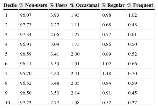
The model is statistically significant according to the Wald test and chi-square likelihood ratio (LR Chi²). Given the net monthly household income for each, we obtain the distribution of cocaine use by income categories summarized in Table 3.

Table 3.

Cocaine use rates by income categories.

Decile	% Non-users	% Users	% Occasional	% Regular	% Frequent
1	96.07	3.93	1.93	0.98	1.02
2	97.73	2.27	1.11	0.68	0.48
3	97.34	2.66	1.27	0.77	0.61
4	96.91	3.09	1.73	0.86	0.50
5	96.59	3.41	2.00	0.89	0.52
6	96.41	3.59	1.91	1.02	0.66
7	95.70	4.30	2.41	1.18	0.70
8	96.52	3.48	2.05	0.84	0.59
9	96.50	3.50	2.14	0.91	0.45
10	97.23	2.77	1.98	0.52	0.27

The prevalence of cocaine use (irrespective of consumption level) among adults in Spain ranges between 2.27% and 4.30% for all income levels. The no/very low income category (the first decile) includes unemployed individuals, who are at a high risk of cocaine use (3.93%). For all the income categories except the first decile, cocaine use increases with income level to peak at 4.30% (2.41%, 1.18%, and 0.70% for occasional, regular, and frequent use, respectively) at 1900 euros per month (decile 7). From this point, prevalence decreases as income rises.

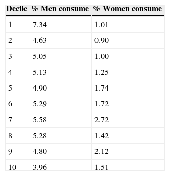
Prevalence of cocaine consumption by sex and by income categories is shown in Table 4.

Table 4.

Cocaine use rates by sex and by income categories.

Decile	% Men consume	% Women consume
1	7.34	1.01
2	4.63	0.90
3	5.05	1.00
4	5.13	1.25
5	4.90	1.74
6	5.29	1.72
7	5.58	2.72
8	5.28	1.42
9	4.80	2.12
10	3.96	1.51

Table 4 confirms a higher rate for men, irrespective of income level. Among individuals aged over 18 years in Spain, rates of cocaine use (whether occasional, regular or frequent) are strikingly different between the sexes, at 3.96–7.34% for men and 0.90–2.72% for women.

3.2

Predictors of cocaine consumption

Here we analyzed which variables or groups of variables (sex, age, marital status, educational level, health perception, employment status, household size and income) could be good predictors of cocaine use for persons aged over 18 in Spain. We examined decision tree rule sets and flows so as to classify and determine risk profiles (see Fig. 2). The decision tree, generated using the CHAID algorithm (Kass, 1980), predicts a risk of 0.033, indicating that the cocaine use categories predicted by the model are incorrect in 3.3% of cases; in other words, the risk of wrongly classifying a cocaine user is 3.3%.

Figure 2.

CHAID decision tree: root, node 2 and two child nodes 7 and 8.

The first branch of the decision tree indicated marital status to be the main predictor variable; this resulted in two nodes, referring to individuals living with a partner (node 1) and single individuals (node 2).

Referring to node 2, of the single individuals (49.0% of the sample), 94.3% are non-users and 3.2%, 1.5% and 1.0% are occasional, regular, and frequent users. Node 2 branches into two nodes representing the sex variable, with men (node 8) indicated as having higher use rates—4.5% (occasional), 2.3% (regular) and 1.5% (frequent)—than women (node 7)—1.7% (occasional), 0.7% (regular), and 0.4% (frequent). Node 8 branches into the nodes representing employment status (nodes 18, 19 and 20), where prevalence of use is higher for (single) men who are unemployed (node 20), at 5.4%, 3.3%, and 2.4% for occasional, regular, and frequent use, respectively; for these men, if they are employed (node 19), the corresponding rates are 4.6%, 2.3% and 1.5%.

The next strongest predictor for cocaine risk is the age variable (nodes 32, 33 and 34), which branches into nodes representing the age groups 18–36 years, 36–44 years and 44–65 years (nodes 32, 33 and 34, respectively). The highest rates of cocaine use—5.3% (occasional), 2.4% (regular) and 1.6% (normal)—correspond to the 18–36 age group (node 32). For age groups over 44 years (nodes 33 and 34), use rates fall significantly (maximum 2.2%).

Node 32 branches into nodes representing education level (nodes 46, 47 and 48: node 47 is no education, node 48 university education and node 46 other), where the highest use rate for single men, aged under 36 years and employed, is when they have basic education levels (node 46). Finally, node 48 (university education) branches into nodes representing the household size variable, where the smallest household size (node 55) is associated with a high use rate.

In short, the decision tree defines a cocaine user profile reflecting the node pattern 0→2→8→19→32→48→55 corresponding to the variables cocaine use→marital status→sex→occupational status→age→education level→household size. The best predictor for cocaine use is marital status. The highest rate of frequent cocaine use (7.1%) is observed among single, unemployed young males with a low education level. Finally, with respect to accuracy, the model correctly classifies approximately 96.7% of individuals and is 100% accurate for the category of non-users.

The decision tree classifies all the individuals in cocaine risk profiles by combining and grouping the explanatory variables. For all levels of consumption (occasional, regular and frequent), we obtain the following three high-risk profiles for cocaine use:

• (1)

  Single men, 25–50 years old, inactive, and with an income of around 1600 euros per month (0.1% of our sample). The prevalence of cocaine use is 18.4%.

• (2)

  Single men, employed, under 36 years old, and with a low education level (1.1% of our sample). The prevalence of cocaine use is 18%.

• (3)

  Single men, unemployed, and with a low education level (0.3% of the sample). The prevalence of cocaine use is 15.7%.

3.3

The impact of socioeconomic and demographic factors

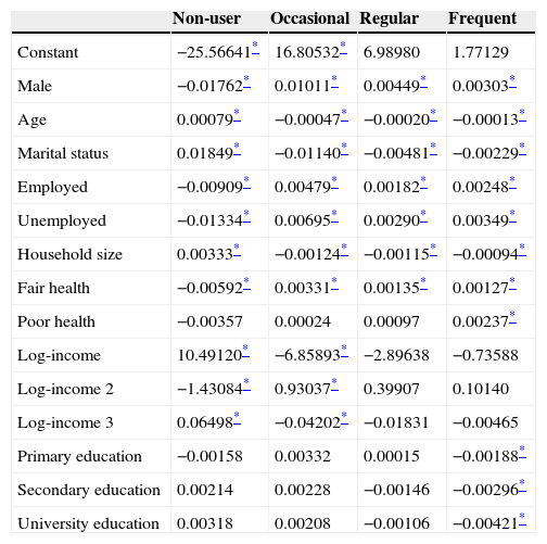
To measure the impact of socioeconomic and demographic determinants of cocaine use in individuals aged over 18 years for each level of use, we calculated multinomial logit regression model coefficients (see Table 5).

Table 5.

Logit regression model coefficients.

	Non-user	Occasional	Regular	Frequent
Constant	−25.56641^*	16.80532^*	6.98980	1.77129
Male	−0.01762^*	0.01011^*	0.00449^*	0.00303^*
Age	0.00079^*	−0.00047^*	−0.00020^*	−0.00013^*
Marital status	0.01849^*	−0.01140^*	−0.00481^*	−0.00229^*
Employed	−0.00909^*	0.00479^*	0.00182^*	0.00248^*
Unemployed	−0.01334^*	0.00695^*	0.00290^*	0.00349^*
Household size	0.00333^*	−0.00124^*	−0.00115^*	−0.00094^*
Fair health	−0.00592^*	0.00331^*	0.00135^*	0.00127^*
Poor health	−0.00357	0.00024	0.00097	0.00237^*
Log-income	10.49120^*	−6.85893^*	−2.89638	−0.73588
Log-income 2	−1.43084^*	0.93037^*	0.39907	0.10140
Log-income 3	0.06498^*	−0.04202^*	−0.01831	−0.00465
Primary education	−0.00158	0.00332	0.00015	−0.00188^*
Secondary education	0.00214	0.00228	−0.00146	−0.00296^*
University education	0.00318	0.00208	−0.00106	−0.00421^*

Notes: Reference categories: Female, inactive, good health, no education.

*

Statistical significance (p < 0.05).

The marital status, sex, age, employment status, and household size variables exert a statistically significant influence on cocaine use in individuals aged over 18 years in Spain. For certain cocaine use categories, furthermore, education, income, and health are also significant.

3.3.1

Sex

The sex variable exerts a statistically significant positive influence on occasional, regular, and frequent cocaine use and a statistically significant negative influence on non-use. Men are far more likely than women to be cocaine users; in particular, being female reduces prevalence of use by 1.8. This result agrees with those reported by Merline et al. (2004) for middle-aged U.S. adults.

3.3.2

Age

Age exercises a statistically significant positive influence on non-use and a statistically significant negative influence on the use categories. The older the individual the less likely they are to use cocaine. One explanation for this pattern is that cocaine is typically consumed in social and leisure settings that tend to be frequented by younger people and younger people are more likely to be drawn to new experiences. Each additional year older increases the likelihood of being a non-consumer by 0.08.

3.3.3

Marital status

Individuals with a partner are less likely to use cocaine than those without a partner. Living with a partner has a statistically significant negative influence on cocaine use (occasional, regular or frequent), increasing the probability of being a non-user by 1.8. These results corroborate those obtained for the USA (Saffer and Chaloupka, 1999) and for the city of New York in particular (Gill and Michaels, 1991). The explanation may be the fact that the negative consequences of cocaine use also affect an individual's partner. Also, if the partner is not a consumer, consumption is likely to be lower, since the partner would have to be excluded.

3.3.4

Employment status

Being unemployed has a statistically significant positive influence on occasional, regular, and frequent cocaine use. The weight of this variable is highest for the occasional use category and corroborates the results of (Royo-Bordonada et al., 1997). By contrast, the influence of unemployment is significant and negative in the case of non-use. This result corroborates those of (Green et al., 2010), who reported, for South Chicago, that unemployed compared to employed adults aged 32–33 years were four times more likely to use cocaine. Being inactive or unemployed means an individual with more leisure hours and, with more opportunities to be alone, he or she has more opportunities to consume drugs.

3.3.5

Household size

The probability of consuming cocaine—most especially on an occasional basis—is reduced in larger households. Normally, households are typically composed of members of different generations and probably include any or all of a partner, siblings, parents or children, so cocaine use may be difficult to share. Living with other people also reduces the risk for cocaine use because individuals may wish to avoid harming the people close to them.

3.3.6

Education

Education level is statistically significant for the frequent use category, with better educated individuals less likely to be frequent users. This result is consistent with results reported for U.S. adults aged 19–50 years studied in the period 1979–2002 (Harder and Chilcoat, 2007). The explanation is that educated individuals typically are more knowledgeable and aware of the repercussions of drug use. Education level has no significant influence on the other use categories, however. Whereas frequent consumption may be interpreted as causing physical and mental deterioration, occasional or regular use may be interpreted as diversion. Better educated individuals usually have more intellectual resources and are more likely to exercise the self-control necessary to avoid becoming addicted to cocaine.

3.3.7

Income

Net monthly household income has a statistically significant positive influence on non-use (Fig. 3) and a statistically significant negative influence on occasional use (Fig. 4). Cocaine non-use is more likely at higher incomes and occasional cocaine use falls as income levels grow. Indeed, a positive correlation between cocaine use and GNP per capita for 62 countries is reported (Saiz, 2007; UNODC, 2005), confirming greater cocaine use in wealthier countries. For a sample of men aged 18–45 years resident in five U.S. States, a statistically significant negative relationship between daily drug use and income level was confirmed (Buchmueller and Zuvekas, 1998). We conclude that once cocaine use becomes regular or frequent, the income variable is no longer statistically significant, as the addicted individual will consume cocaine irrespective of their income.

Figure 3.

Impact of household income on non-use of cocaine.

Figure 4.

Impact of household income on occasional use of cocaine.

3.3.8

Health perception

For individuals who perceive their health to be fair, the probability of being a non-user is lower by 0.6 and the probability of being an occasional, regular or frequent user is higher by between 0.1 and 0.3. Individuals who perceive their health to be good tend not to be cocaine users, as they are probably fully aware of the implications for health. Similarly, if health is perceived to be poor, then frequent cocaine use is higher, probably for the same reasons.

4

Conclusions

In this paper we analyzed the socioeconomic determinants of cocaine use by adults aged over 18 years in Spain in order to profile the population segments at greatest risk. We report a prevalence of cocaine use (whether occasional, regular or frequent) in Spain of 3.3%, one of the largest all over the world.

Decision tree analysis yielded information on factors with greater predictive power and enabled us to classify high-risk cocaine use profiles. A CHAID-type classification tree indicated the main predictors to be marital status, sex, employment status, age, education level, and household size.

The individuals at greatest risk were indicated to be (1) single men, inactive, 25–50 years old, and with an income of around 1,600 euros per month; (2) single men, employed, under 36 years old, and with a basic education; and (3) single men, unemployed, under 36 years old, and owning a basic education. Prevalence rates for these profiles were 18.4%, 18.0% and 15.7%, respectively. These three groups accounted for 1.5% of our sample.

Multinomial logistic regression indicated the determinants for occasional, regular, and frequent cocaine use to be sex (positive for men), marital status (negative for having a partner), employment status (positive for unemployment), household size (negative for a larger household), and age (negative for older age groups, with prevalence falling in line with increasing age). In addition, higher education levels are associated with lower levels of frequent use. Finally, individuals who perceive their health to be poor have a higher rate of frequent cocaine use.

Monthly net household income has a statistically significant effect on non-use and occasional use. The higher the income level, the higher the probability of non-use and the lower the probability of occasional use. No significant differences were observed according to income levels, however, for regular and frequent use. When consumption acquires a certain frequency and the individual becomes addicted, it would appear that income is no longer a determining factor.

Globally, our results would suggest that cocaine prevention and education campaigns in Spain should be reoriented to focus on single men aged under 36 years with a low education level living in small, low-income households. Understanding fully the consequences of cocaine use for an individual's own health and for their family may be decisive in the choice to use cocaine. Note that, in terms of communicating with the population, responses from the most recent EDADES survey of 2011 indicated that 51% and 36.2% of respondents expressed a preference for receiving information on drug use through the media and through the Internet (website, social networks, forums, etc.), respectively.

Funding

M. Antelo and J. C. Reboredo acknowledge funding from the Xunta de Galicia and FEDER via research programme GPC2013-045.