

En este trabajo se analiza la relación empírica entre las emisiones de dióxido de carbono (CO2) per cápita y el crecimiento económico en un panel de 20 países de América Latina y el Caribe durante el periodo 1971-2011. Dicha relación empírica, conocida en la literatura económica como la hipótesis de la curva de Kuznets ambiental (CKA), sugiere que la relación entre ambas variables tiene en el largo plazo una relación funcional en forma de U-invertida, es decir, a partir de cierto nivel de renta per cápita, un mayor crecimiento económico iría acompañado de mejoras en la calidad ambiental. Si bien esta hipótesis ha sido estudiada desde la década de 1990, recientemente su validez empírica ha sido cuestionada, entre otras cosas, por la falta de análisis de estacionariedad de las variables, y en un contexto de datos panel, la presencia de dependencia cruzada. Tomando en cuenta ambas críticas, empleamos novedosas pruebas de raíces unitarias y técnicas de cointegración robustas para la presencia de dependencia en el panel. Encontramos resultados contradictorios dependiendo del supuesto de dependencia cruzada entre los países. Bajo el supuesto de independencia cruzada, se confirma la existencia de una CKA con puntos de quiebre realistas. Sin embargo, dicho supuesto es rechazado posteriormente, concluyendo así que en presencia de dependencia cruzada en el panel, no se puede establecer una relación de equilibrio a largo plazo entre las variables, i.e., se rechaza la existencia de una CKA.
This paper analyzes the empirical relationship between carbon dioxide (CO2) emissions per-capita and economic growth in a panel of 20 Latin American and Caribbean countries over the period 1971-2011. This empirical relationship, known in the economic literature as the Environmental Kuznets Curve (EKC) hypothesis, suggests that the relationship between these variables, in the long run, follows an inverse U-shape, that is, from a certain level of per-capita income, an increased economic growth would be accompanied by improvements in environmental quality. Although this hypothesis has been studied since the 1990s, its empirical validity has recently been questioned on the basis of, among other things, the lack of diagnosis of the stationarity properties of the variables, and in a panel data context, the presence of cross-sectional dependence. Taking into account both criticisms, we use recent unit root tests and cointegration techniques that are robust to the presence of cross-sectional dependence. We find contradictory results depending on the assumption of cross-dependence. Under the assumption of cross-independence, the existence of an EKC with a realistic turning point is confirmed. However, this assumption is subsequently rejected, and because of the presence of cross-dependence in the panel, a long-run equilibrium relationship between the variables cannot be established, and we reject the existence of an EKC.
The relationship between economic growth and environmental pollution is considered one of the most important empirical relationships in environmental economics, having as one of its main assumptions that in a country's development process, as per-capita income rises, environmental quality initially deteriorates to a certain point, after which environmental quality improves while income continues to rise. Graphically, this empirical relationship takes the form of an inverted U-shape, and is known in the economic literature as the Environmental Kuznets Curve (EKC). The intuition behind the EKC follows from three key effects that determine the relationship between economic growth and environmental quality during the process of development: i) the scale effect, states that an increase in production demands more inputs, which implies higher emissions of pollutants; therefore, it is said that economic growth has a negative impact on the environment; ii) composition effect, as the economy grows, its structure could change, consequently there may be greater participation of cleaner or dirtier activities, thus it is said that the composition effect has an ambiguous effect on environmental quality; iii) technique effect, suggests that changes in the level of per-capita income can induce changes in civil environmental preferences, for example, an increase can lead the preferences towards higher environmental quality, which may lead to changes in environmental policies, which in turn can have an effect on production methods, directing them towards the use of less polluting technologies (Grossman and Krueger, 1995; Panayotou, 1997).
From an optimistic point of view, the EKC hypothesis suggests that economic growth is, by itself, the solution to environmental problems in the sense that environmental improvement is almost an inevitable consequence of economic growth, and thus, when a country becomes richer, current environmental problems will be addressed by policy changes that not only protect the environment, but also promote economic development (Roca et al., 2001; Perman and Stern, 2003). However, this is a very simplistic conclusion, since environmental degradation is not explained solely by the current emissions rates or pollutant concentrations, but also depends on past environmental pressures, and as Arrow et al. (1995) conclude, “… economic growth is not a panacea for environmental quality; indeed is not even the main issue”.
The empirical literature on the analysis of the EKC emerged during the early 1990s with the study by Grossman and Krueger (1991), who in the context of the North American Free Trade Agreement (NAFTA) found an inverted-U relationship between some pollutant emissions such as sulfur dioxide or smoke and per-capita income for the US previous to the NAFTA. Shafik and Bandyopadhyay (1992) estimated EKCs for ten indicators of environmental degradation for 149 countries over the period 1960-1990, and found an inverted-U relationship between income and ambient concentrations of air pollutants. In the Latin American context, Poudel et al. (2009) tested for EKC in the greenhouse gas carbon dioxide (CO2) in 15 Latin American countries over the period 1980-2000. They do not find an inverted U-relationship, but instead, their results show an N-shaped curve for the region.
However, the empirical validity of the early EKC studies mentioned above has been questioned by some (for further discussion see Borghesi, 2001; Stern, 2004; Galeotti et al., 2006; Romero-Ávila, 2008) on the basis of the sensitivity of the results to variations in model-specification, the lack of diagnosis of the stationarity properties of the variables, and the assumption of cross-sectional independence, and the possible presence of structural breaks in the long-run relationship implied by the EKC hypothesis.
Regarding the first issue, the stationarity properties of the variables, let us remember that a time series is said to be stationary if all its statistical properties such as mean, variance, autocorrelation, and so on, remain constant over time; in contrast, in non-stationary processes, the statistical properties change over time. A non-stationary process that needs to be differenced d times before it becomes stationary is said to be integrated of order d or I(d). A stationary process of order 0 or I(0) is integrated, known as stationary level. The idea behind testing the stationarity properties of the variables is to avoid unreliable and spurious regressions, since by rule, non-stationary variables are unpredictable, the estimation results might indicate a relationship between variables where one does not exists (Phillips, 1986). The panel unit root tests (PURTs), which are used to test for stationarity, can be divided into two categories according to their cross-section dependence assumption: the so called first generation assume cross-section independence, while the second generation allow for cross-section dependence between the cross-section units.
There are a number of studies that test for the order of integration of the variables. Al-mulali et al. (2015), for example, study the effect of economic growth, renewable energy consumption and financial development on CO2 emissions in a panel of 18 Latin American and Caribbean (LAC) countries over the period 1980-2010. Their results confirm the existence of an EKC. Apergis and Ozturk (2015) test the EKC for 14 Asian countries from 1990-2011, including as regressors a variety of economic and policy related variables. Their results support the EKC hypothesis. Al-mulali and Ozturk (2016) analyze the role of energy price in air pollution for a panel of 27 countries over 1990-2012, finding evidence of the EKC hypothesis. Bilgili et al. (2016), including as regressors renewable energy consumption for 17 countries that belong to the Organisation for Economic Co-operation and Development (OECD) over the period 1977-2010, obtain results that confirm the existence of the EKC.
Regarding the second issue, the assumption of cross-sectional independence in the panel is rather restrictive and somewhat unlikely to hold since co-movement of economies are often expected yielding cross-sectional dependence as a consequence of spatial effects, regional and macroeconomic linkages, unobserved common factor and externalities (O’Connel, 1998; Phillips and Sul, 2003). In order to overcome this deficiency, a second generation of panel unit root and cointegration tests, considering the cross-sectional dependence between the cross-section units, has been developed. Using this technique, Wagner (2008) compares the first and second generation unit root tests on a data set for 100 countries over the period 1950-2000. His results are very dependent on the type of test chosen, i.e., when his estimations do not account for cross-sectional dependence they confirm the EKC hypothesis, whereas accounting for cross-sectional dependence, he finds no significant evidence in favor of the EKC hypothesis. Arouri et al. (2012), including energy consumption in the regression equation, find no evidence of EKC relationship for 12 Middle East and North African countries over the period 1981-2005. Apergis (2016) tests the EKC for 15 OECD countries over the period 1960-2013, finding evidence of a long-run relationship between emissions and income. Dogan and Seker (2016), testing for the European Union over the period 1980-2012, with renewable and non-renewable energy, real income and trade openness as regressors, find support for the EKC hypothesis.
The presence of structural breaks, which can arise due to external shocks, financial crisis, and technological progress, etc., has been tested by Romero-Ávila (2008), who analyze the existence of an EKC for a sample of 86 countries over the period 1960-2000. He finds that CO2 emissions are non-stationary while the Gross Domestic Product (GDP) appears to be stationary around a broken trend. He points out that this result has implications when modelling the EKC since a different order of integration invalidates the cointegration techniques which assumes that both variables are non-stationary and cointegrated one with another. Jaunky (2011) test the EKC for 36 high-income countries over the period 1980-2005, controls for structural breaks in the unit root tests, finding no evidence of an EKC.
In general, the results of the empirical literature are not conclusive about the existence of an EKC, nor the particular form of the relationship between economic growth and CO2 emissions, also the results are quite sensitive to the functional form used in the regression equation, the sample of countries and to the time period considered (Selden and Song, 1994; Borghesi, 2001).
This paper contributes to filling the gap in literature on the understanding of the empirical relationship between CO2 emissions and economic growth in the Latin American context assessing the effects of using appropriate unit root tests and cointegration techniques when cross-sectional dependence is presented in the panel. Unlike the vast majority of the studies mentioned above, we focus entirely on the standard formulation of the EKC, i.e., we examine the effects of per-capita real income and its square on the levels of per-capita CO2 emissions without the inclusion of an energy consumption/use variable as an additional regressor. We exclude this variable since the main source of CO2 emissions is fossil fuel combustion, and burning fossil fuels releases energy from which CO2 is produced as a by-product. Thus the two variables (CO2 emissions and energy use) can be seen as coupled variables (i.e. one variable either directly or indirectly contains the whole or components of the second variable), that if included in the regressions equation, can lead to erroneous results and invalid conclusions (Archie, 1981).
2MethodologyFollowing the literature review on the EKC, we analyze the relationship between environmental quality and economic growth based on the following regression model:
where CO2 stands for per-capita carbon dioxide emissions, Y is the per-capita real GDP and εit is the error term, it denotes the observation on the i-th cross-section unit at time t, for t = 1,2,...,T and i = 1,2,...N.
In equation (1), if the EKC hypothesis holds, β1 > 0 and β2 < 0 and both must be statistically significant, so that the pollution curve eventually turns down. In this case, the turning point with respect to income is given by yturning_point = exp(– β1/2 β2).
Following the discussion of the stationarity properties of the variables and cross-dependence in the panel, for comparison purposes, we analyze the relationship with both, the first and second generation PURTs and cointegration techniques. Section 2.1 presents the first generation PURTs, while section 2.2 presents the second generation PURTs.
2.1Assuming cross-country independenceIn order to analyze the order of integration of the variables, we employ six different PURTs. Briefly describing them, let us consider the following first-order autoregressive, AR(1), process:
where i = 1,...,N are the cross-section units in the panel; t = 1,...,T denotes the time and the errors εit are assumed to be independent and identically distributed (IID). (2) can be re-written as a simple Dickey-Fuller (DF) regression:where Δ yit = yit – yi,t–1, ϕi= αi –1. The null hypothesis (non-stationarity) is:


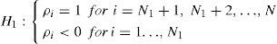
The alternative hypothesis depends on the persistence of the autoregressive parameter. If the autoregressive parameter is assumed to be common for all the cross section units, the process is known as a common unit root process, and the homogeneous alternative is: H1a : ϕ1 = ··· = ϕNϕ and ϕ < 0. Levin et al. (2002), Breitung (2000) and Hadri (2000) tests are based on this form. On the other hand, if the autoregressive parameter vary across cross-sections, the process is called an individual unit root process, and the heterogeneous alternative is:H1b:ϕ1<0,…,ϕNo<0,≤N0≤N. That is, N0 of the N (0 < N0 ≤ N)panel units are stationary with individual specific autoregressive coefficients. The Im, Pesaran and Shin (IPS) (Im et al., 2003), the Fisher-augmented DF (ADF) (Maddala and Wu, 1999) and the Fisher, Phillips and Perron (Fisher-PP) (Choi, 2001) tests follow this form.
The LLC considers the following ADF regression:
where Δ is the first difference operator, yit is the dependent variable, εit is a white-noise disturbance with variance σ2, i = 1,...,N, indexes the countries and t = 1,..., T indexes time. The null hypothesis H0: αi = 0 (unit root) versus H1: αi < 0 with α = ρ – 1 (yit stationary). This test is based on the statistics tβi=βˆi/σβˆi, where βˆi is the OLS estimate of βˆi in equation (5) and σβˆi is its standard error.
The Breitung (2000) test considers the possibility that heteroskedasticity might exists in the sample with the following equation:

The null hypothesis is: H0:∑k=1p+1βik−1=0, whereas the alternative hypothesis assumes that the panel series is stationary, i.e. H0:∑k=1p+1βik−1<0 ∀ i.
The main difference between LLC test and the Breitung test is that the former requires a bias correction factor to correct for cross-sectionally heterogeneous variance to allow for efficient pooled OLS estimation, while the Breitung test achieves the same result by the appropriate transformation of variables (Narayan and Smyth, 2008).
The Hadri test, unlike the previous tests, has as null hypothesis stationarity in all units against the alternative of a unit root in all panel members. Hadri's (2000) statistics can be written as:
where σˆϵ2 is the consistent Newey and West (1994) estimate of the long-run variance of disturbance terms.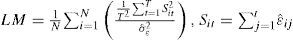
The IPS test is based on ADF test statistics over the cross-sectional units, while allowing for different orders of serial correlations, i.e., it allows for heterogeneous coefficients:

With the null hypothesis that all the individuals follow a unit root process: H0:ρi=0 ∀i versus the alternative that some (but not all) have unit roots:
The Fisher-ADF and Fisher-PP tests use Fisher's (1932) results to derive the p-values from individual unit root tests. Both tests have as the null hypothesis a unit root for all i.
Once tested for stationarity, the next step in the analysis is to test the long-run relationship between the variables. We perform two panel cointegration tests: Pedroni (1999, 2004) and Kao (1999).
Pedroni (1999, 2004) introduces seven panel cointegration statistics based on both homogeneity and heterogeneity assumptions. Assuming a panel of N countries, T observations and m regressors (Xm), the cointegration test follows the equation:
where yi,t and Xj,it are assumed to be integrated of order one in levels, i.e. I (1).
The seven statistics can be divided into two sets. The first one consists of four panel statistics (pooled or within dimension): a) the panel variance-statistics, b) the panel ρ-statistics, c) the panel PP-statistics and d) the panel ADF-statistics. The second set consists of three group panel statistics (between dimension): e) the group ρ-statistics, f) the group PP-statistics and g) the group ADF-statistics.
Under the null hypothesis, all seven tests indicate the absence of cointegration H0:ρi=0 ∀i, whereas the alternative hypothesis is given by H0:ρi=ρ <1 ∀i; where ρi is the autoregressive term of the estimated residual under H1 given by ξˆit=ρiξˆi,t−1+ui,t
In the case of panel statistics, the first-order autoregressive terms is assumed to be the same across all the cross-sections, while in the case of group panel statistics, the parameter is allowed to vary over the cross-sections. The interpretation of the rejection of the null hypothesis of no cointegration differs on the two approaches. If the null is rejected in the panel statistics, it means that the variables are cointegrated for all the cross-sections. On the other hand, if the null is rejected in the group panel statistics, it implies that there is at least one cointegration relationship among the cross-sections.
The Kao test follows the same approach as the Pedroni test, but is based on the assumption of homogeneity across panels with:
where i = 1,...,N ; t = 1,...,T; αi = individual constant term; β = slope parameter and ωi=stationary distribution; Xit and Yit are integrated processes of order I(1) for all i. Kao (1999) derives two (DF and ADF) types of panel cointegration tests. Both tests can be calculated from:
andwhere ω¯it−1 is obtained from the equation (10). The null hypothesis is H0: ρ = 1 (no cointegration), while the alternative hypothesis is H1: ρ < 1.

Once the variables are found to be cointegrated, the next step is to estimate the long-run coefficients. Since the use of non-stationary variables in ordinary least squares (OLS) can lead to spurious regressions, we employ two different approaches. The first one is the Group Mean Fully Modified OLS (GM-FMOLS) proposed by Pedroni (2001, 2004), which is a non-parametric estimation that corrects the standard OLS for bias induced by endogeneity and serial correlation between regressors and residuals and is less sensitive to possible bias in small samples. The second approach is the Group-Mean Dynamic OLS proposed by Pedroni (2001), which averages the estimates obtained from the conventional DOLS estimator applied to the i-th country of the panel. According to Pedroni (2001) the advantage of GM-DOLS is that it is a more flexible model due to allowing for heterogeneous cointegration vectors and appears to suffer much lower small-sample size distortion than the within-dimension estimators.
2.2Accounting for cross-country dependenceIn order to test the null hypothesis of cross-section independence, we employ the Pesaran (2004) CD test. The null hypothesis of cross-section independence is H0: ρij= ρji = (εit, εjt) = 0 for i ≠ j, while the alternative H1: ρij= ρji for some i ≠ j. The test is given by:
where ρˆij is the sample estimate of the pair-wise Pearson's correlation coefficients of the residuals from ADF-type regression:
If cross-sectional dependence cannot be rejected, we apply three different second generation PURTs: the Cross-sectionally ADF (CADF) of Pesaran (2007), the Cross-sectional augmented IPS (CIPS) proposed by Pesaran (2007) and the MP test proposed by Moon and Perron (2004). All these tests have in common the assumption of cross-sectional correlation due to the presence of unknown common factors (e.g. omitted common variables or external shocks affecting the panel members) and specify that the data are generated by a deterministic, idiosyncratic and common component, but their data generating process (DGP) differ with respect to the allowed number of common factors (r). The Pesaran-CADF (PES-CADF) and CIPS tests assume r = 1 (i.e., the error term has an unobserved one-common factor structure accounting for cross-sectional dependence) and the MP test assumes r > 1 (Carrion-i-Silvestre and German-Soto, 2008; Gengenbach et al., 2009).
Pesaran (2007) suggests a Cross-sectionally Augmented Dickey-Fuller test (PES-CADF) where the standard Dickey-Fuller (DF) regressions are augmented with cross-sectional averages of lagged levels and first differences of the i-th cross-section in the panel:
where y¯t−1=1N∑i=1Nyi,t−1,Δy¯t=1N∑i=1Nyit and ti(N,T) is the t-statistic of the estimate of ρi in the above equation used for computing the individual ADF statistics.
The CIPS is a simple average of individual CADF statistics:
where ti(N,T) is the CADF for the i-th cross-section unit given by the t-ratio of ρi in the CADF regression. Both tests have as null hypothesis homogeneous unit root (all individuals within a panel data are non-stationary) versus the alternative that at least one individual in the panel is stationary.
Moon and Perron (2004) develop a factor model test with two modified t-statistics with standard normal distribution for the null hypothesis of a unit root H0:δi=1 ∀ i=1,…,N which is tested against the heterogeneous H1: δi < 1 for some i. The test assumes that the error term follows a K-unobserved-common factors model to which an idiosyncratic shock is added. The number of factors are estimated with Bai and Ng (2002) criteria, in particular with the modified Bayes Information Criterion (BIC) (called BIC3). We choose this criterion because according to Moon and Perron (2007), the criterion performs better in selecting the number of factors when min(n,T) is small (≤ 20).
The long-run relationship between the variables is analyzed with the Westerlund (2007) cointegration test, which includes cross-section dependence in the cointegration equation. This test assumes the following data generating process:
where t = 1.,...,N and i = 1,...,N index the time-series and cross-section units respectively, and dt contains the deterministic components, typically these elements include a constant and a linear trend; to allow for this, there are three different cases. In the first case,dt = 0, so Δyit has no deterministic terms (this is the most restrictive case); in the second case, dt = 1 so Δyit is generated with a constant (the deterministic component is an individual intercept); in the third case, dt = (1,t)’ so Δyit is generated with both a constant and a trend.
The test deal with any dependence across i by using the bootstrap method approach used by Chang (2004). The previous equation (17) can be re-written as:
where λ′i=−αiβ′i. The parameter αi determines the speed at which the system corrects back to the equilibrium relationship yi,t−1−β′i xi,t−1 after a sudden shock. Thus, the null hypothesis of no cointegration can be implemented as H0:αi=0∀i. The alternative hypothesis depends on what is being assumed about the homogeneity of αi. The two tests presented, the so called group-mean tests, do not require the αis to be equal, which means that H0 is tested versus H1g:αi<0 for at least one i, suggesting that a rejection should be taken as evidence of cointegration for at least one of the cross-sectional units. The second pair of tests, called panel tests (which are based on pooling the information regarding the error correction along the cross-sectional dimension of the panel), assume that αi is equal for all i and are, therefore, designed to test H1p:αi=<0∀i vs. H0, suggesting that a rejection should be taken as evidence of cointegration for the panel as a whole.2.3Data
We focus our analysis on 20 Latin American and Caribbean (LAC) countries over the period 1971-2011. Per-capita CO2 emissions and real GDP per-capita were obtained from the 2015 World Development Indicators. Table I shows the descriptive statistics of the panel. Table IA country statistics are shown.
Descriptive statistics of the variables for 20 Latin American and Caribbean countries.*
| Variable | Unit | Mean | Standard deviation | Min | Max |
|---|---|---|---|---|---|
| CO2 | metric tons | 1.9675 | 1.4168 | 0.25022 | 7.611 |
| GDP | 2005 USD | 3297.614 | 1763.614 | 743.805 | 9085.243 |
First we show the results assuming that the countries are cross-independent. In the second part, the results accounting for cross-dependence are presented.
3.1First generation panel testsThe order of integration of the variables is analyzed with six different PURTs. According to the results shown in Table II, all the variables are non-stationary in levels, while becoming stationary in first differences, thus both variables are I(1). The results are robust to the inclusion of a trend in the PURT equation.
Panel unit root tests results.
| Variable | LLC | IPS | ADF-FISHER | PP | ||||
|---|---|---|---|---|---|---|---|---|
| Intercept | Intercept and trend | Intercept | Intercept and trend | Intercept | Intercept and trend | Intercept | Intercept and trend | |
| lnCO2 | –1.1515 (0.1247) | –0.056 (0.4776) | 0.2186 (0.5865) | 0.4574 (0.6763) | 40.5214 (0.4473) | 38.4823 (0.5386) | 43.7442 (0.3155) | 34.7054 (0.7071) |
| lnY | 1.8185 (0.9655) | 1.770 (0.9616) | 3.7232 (0.999) | 0.3885 (0.6512) | 27.6464 (0.9305) | 47.5090 (0.1933) | 21.3720 (0.9931) | 21.1399 (0.9679) |
| (ln(Y))2 | 2.3485 (0.9906) | 1.8026 (0.9643) | 4.1421 (1.000) | 0.6555 (0.7439) | 25.4330 (0.96459 | 45.6104 (0.2502) | 19.2156 (0.9978) | 23.3899 (0.9832) |
| ΔlnCO2 | –19.000 (0.000) | –16.9723 (0.000) | –18.0486 (0.000) | –16.9723 (0.000) | 368.753 (0.000) | 328.818 (0.000) | 532.939 (0.000) | 1147.13 (0.000) |
| ΔlnY | –11.8063 (0.000) | –10.9514 (0.000) | –11.7166 (0.000) | –10.3647 (0.000) | 222.490 (0.000) | 180.917 (0.000) | 235.474 (0.000) | 179.744 (0.000) |
| Δ(ln(Y))2 | –11.7524 (0.000) | –10.4152 (0.000) | –11.6384 (0.000) | –10.0295 (0.000) | 220.725 (0.000) | 175.476 (0.000) | 236.103 (0.000) | 179.988 (0.000) |
| Variable | Breitung Intercept and trend | Hadri Intercept | Breitung ntercept and trend | Hadri Intercept | ||||
| lnCO2 | 0.7134 (0.7622) | 12.2019 (0.000) | ΔlnCO2 | –10.3285 (0.000) | 0.3932 (0.3471) | |||
| lnY | 0.5236 (0.6997) | 14.1492 (0.000) | ΔlnY | –7.7994 (0.000) | 1.8293 (0.0337) | |||
| (ln(Y))2 | 0.5560 (0.7109) | 14.4054 (0.000) | Δln2Y | –6.7542 (0.000) | 1.9193 (0.0275) | |||
Note: All the tests have as H0: non-stationarity, except for Hadri, which has as null stationarity; lag lengths were selected automatically using the Akaike information criterion (AIC); p-values are in parentheses.
Once we found that both variables are I(1), we perform cointegration tests to look for a long-run relationship among the variables. Table III shows the results of Pedroni (1999, 2004) and Kao (1999) tests. In the Pedroni test when an intercept and a trend are included as deterministic components, the null hypothesis of no cointegration is rejected for three of the four tests for the panel statistics and for two of the three test in the group statistics.
Cointegration tests results.
| Pedroni residual cointegration test | ||
|---|---|---|
| Trend assumption | Deterministic intercept and trend | No deterministic trend |
| Alternative hypothesis: common AR coefficients (within-dimension) | ||
| Panel v-statistics | –0.2156 (0.6239) | –0.4167 (0.6615) |
| Panel rho-statistics | –1.8667 (0.0310) | –0.2009 (0.4204) |
| Panel PP-statistics | –3.6696 (0.0001) | –1.1116 (0.1331) |
| Panel ADF-statistics | –3.0312 (0.0012) | –1.6239 (0.0522) |
| Alternative hypothesis: individual AR coefficients (between-dimension) | ||
| Group rho-statistics | –0.7199 (0.2358) | 0.876140 (0.8095) |
| Group PP-statistics | –3.5267 (0.0002) | –0.4590 (0.3231) |
| Group ADF-statistics | 3.2235 (0.0006) | –2.4660 (0.0068) |
| Kao residual cointegration test | ||
| ADF | t-Statistic | Prob |
| –2.5042 | 0.0061 | |
Note: H0: no cointegration. Automatic lag length selection based on AIC criterion. Newey-West automatic bandwith selection and Bartlett kernel.
For the model with only a constant (intercept), we can reject the null of no cointegration for one of the four panel statistics, and for one of the three group statistics. Although these results are not robust to the inclusion of a trend in the cointegration equation, we follow Pedroni (1999), who points out that the panel non-parametric (t-statistics) and parametric (ADF-statistics) statistics are more reliable in a constant plus trend, thus in general we can conclude that there is cointegration among the variables in the panel. The Kao test strongly rejects the null of no cointegration. With the results of both tests, we can conclude that per-capita CO2 and per-capita GDP are moving together in the lon grun.
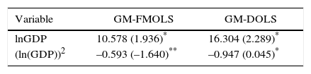
The long run equilibrium relationship is estimated with the Group-Mean Fully Modified OLS (GM-FMOLS) and the Group-Mean Dynamic OLS (GM-DOLS) by Pedroni (2000, 2001). Results of the estimation are reported in Table IV.
Since both estimations are statistically significant, with positive coefficients on income per-capita and negative coefficients on income per-capita squared, the existence of an EKC is confirmed. According to the GM-FMOLS, an increase of 1% in real per-capita GDP increases emissions by approximately 11% and an increase of 1% in the square of real per-capita GDP decreases emissions by 0.59%. The same interpretation can be given to the GM-DOLS, an increase of 1% in real per-capita GDP increases emissions by 16% and an increase of 1% in the squared of real percapita GDP decreases emissions by 0.95%.
Based on this estimations, the turning point of the per-capita CO2 emissions would occur at a per-capita income level of 7,437 USD for the GM-FMOLS. Argentina, Chile and Mexico already reached this level. For the GM-DOLS, the estimated turning point is at USD5,476. Argentina, Brazil, Chile, Costa Rica, Cuba, Mexico, Panama, Uruguay and Venezuela already reached this level.
3.2Second generation panel testsThe result in Section 3.1 were reached under the assumption of cross-sectional independence in the panel. However, since the assumption is quite restrictive an unlikely to happen, in this section we present the results accounting for cross-sectional dependence in the panel.
First we investigate the presence of cross-section dependence in the panel with the Pesaran (2004) CD test. The results of the test strongly reject the null hypothesis of cross-sectional independence in the panel. The result of the CD test for (1) is 8.09 (p = 0000). The results of the CD test computation for the individual variables are 31.194 and 46.452 for CO2 and GDP, respectively.
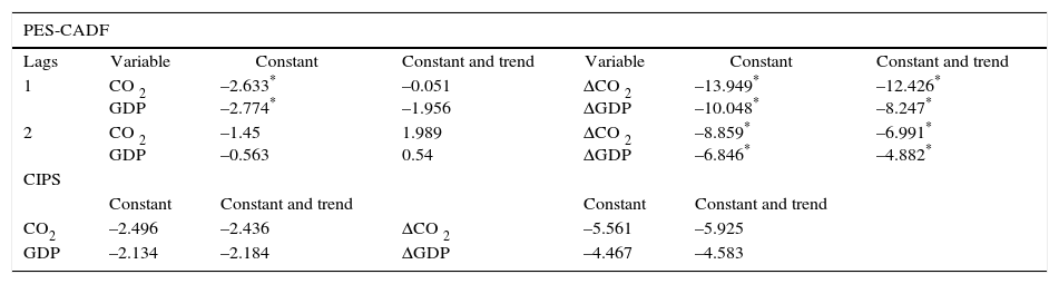
The results of the three PURTs are presented in Table V and Table VI. We find contradictory results depending on the way cross-section dependence is accounted for. If it is assumed to occur due to a single common factor, the PES-CADF and CIPS tests do not reject the null hypothesis of a unit root.
Unit root tests results.
| PES-CADF | ||||||
|---|---|---|---|---|---|---|
| Lags | Variable | Constant | Constant and trend | Variable | Constant | Constant and trend |
| 1 | CO 2 GDP | –2.633* –2.774* | –0.051 –1.956 | ΔCO 2 ΔGDP | –13.949* –10.048* | –12.426* –8.247* |
| 2 | CO 2 GDP | –1.45 –0.563 | 1.989 0.54 | ΔCO 2 ΔGDP | –8.859* –6.846* | –6.991* –4.882* |
| CIPS | ||||||
| Constant | Constant and trend | Constant | Constant and trend | |||
| CO2 | –2.496 | –2.436 | ΔCO 2 | –5.561 | –5.925 | |
| GDP | –2.134 | –2.184 | ΔGDP | –4.467 | –4.583 | |
Notes: H0: homogeneous non-stationary; lag criterion decision: general to particular based on F joint test; critical values, CIPS with constant: 10% (–2.03), 5% (–2.11), 1% (–2.25); critical values CIPS with constant and trend: 10% (–2.54), 5% (2.62), 1% (–2.76);
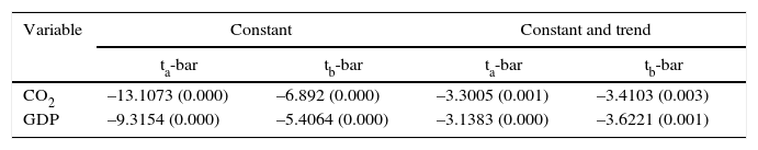
Moon and Perron unit root test results.
| Variable | Constant | Constant and trend | ||
|---|---|---|---|---|
| ta-bar | tb-bar | ta-bar | tb-bar | |
| CO2 | –13.1073 (0.000) | –6.892 (0.000) | –3.3005 (0.001) | –3.4103 (0.003) |
| GDP | –9.3154 (0.000) | –5.4064 (0.000) | –3.1383 (0.000) | –3.6221 (0.001) |
Notes: Maximum number of potential common factors: five; criteria used to estimate the number of common factors: BIC3; common factors estimated: two.
On the other hand, when cross-dependence is assumed to occur due to one or more common factors, MP test strongly rejects the null of non-stationarity.
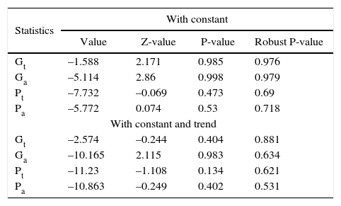
Having established that the variables are I(1), the Westerlund (2007) cointegration test, shown in Table VII, fails to reject the null hypothesis of no cointegration between per-capita CO2 emissions and per-capita real GDP for all the statistics. Regardless of the specification of the deterministic component considered, we can conclude that there is no long-run equilibrium relationship between the variables when we consider cross-dependence in the panel.
Westerlund cointegration test results.
| Statistics | With constant | |||
|---|---|---|---|---|
| Value | Z-value | P-value | Robust P-value | |
| Gt | –1.588 | 2.171 | 0.985 | 0.976 |
| Ga | –5.114 | 2.86 | 0.998 | 0.979 |
| Pt | –7.732 | –0.069 | 0.473 | 0.69 |
| Pa | –5.772 | 0.074 | 0.53 | 0.718 |
| With constant and trend | ||||
| Gt | –2.574 | –0.244 | 0.404 | 0.881 |
| Ga | –10.165 | 2.115 | 0.983 | 0.634 |
| Pt | –11.23 | –1.108 | 0.134 | 0.621 |
| Pa | –10.863 | –0.249 | 0.402 | 0.531 |
H0: no cointegration; lags and lead automatically selected by AIC criterion with Bartlett-Kernel window width set according to 4(T/100)2/9 ≈ 3; robust p-value controls for cross-section dependence; bootstrap 800; test performed with the xtwest command in Stata by Persyn and Westerlund (2008).
The aim of this research is to test the empirical relationship between CO2 emissions and economic growth for a panel of 20 Latin American and Caribbean countries over the period 1971-2011, with a wide variety of unit root and cointegration tests.
Our main contribution to the literature is the re-analysis of the classic EKC hypothesis (i.e., not including any additional explanatory variable besides GDP) for Latin American countries employing a set of novelty unit root and panel cointegration tests. Following Stern (2004) who points out that most of the early EKC literature is econometrically weak and the common assumption of cross-dependence can lead to biased results (Aslanidis, 2009; Wagner, 2008), we apply the so-called first and second generation panel unit root and cointegration test and compare the results in two different sections of the paper.
In the first one, all the six PURTs employed confirm that the variables are integrated of the same order (I[1]) and cointegrated, indicating that there is a stable equilibrium relationship between carbon dioxide emissions and GDP. The panel GM-FMOLS and GM-DOLS confirm the existence of and EKC with plausible turning points at USD7437 and USD5476, respectively. However, we need to remember that in this so-called first generation unit root and cointegration tests the common assumption is that all cross-sections are independent, i.e. assumes that CO2 emissions and GDP are independent across countries, which is something highly unlikely to hold in practice.
In the second part of the analysis, the presence of cross-dependence in the panel is detected. The PURTs show that CO2 emissions are integrated of order one but are not cointegrated. As the model does not satisfy cointegration properties, any further attempt to estimate an EKC will give unreliable results.
Overall, our mixed results confirm the high sensitivity of EKC hypothesis to empirical methodology employed and contribute to the debate that despite the approach considered, there is no clear evidence of existence of an EKC for carbon emissions. We highlight the importance of controlling for cross-sectional dependence in the panel, which occurs due to unobserved common factors which seems to be a very decisive link in the environmental quality-economic growth relationship.
Finally, future studies could extend these results with further analysis of the unobserved common factors. Also, it is worth mentioning that in this study we did not take into consideration the possible presence of structural breaks, thus it is recommended to re-analyze the EKC hypothesis taking into account possible structural breaks.
Descriptive statistics: real per-capita GDP in 2005 USD.
| Country | Mean | Std. Dvs | Minimum | Maximum |
|---|---|---|---|---|
| Argentina | 5180.63 | 777.21 | 3918.89 | 7590.07 |
| Bolivia | 965.35 | 116.13 | 780.57 | 1247.84 |
| Brazil | 4154.56 | 671.24 | 2547.44 | 5744.46 |
| Chile | 5088.78 | 2106.39 | 2543.17 | 9085.24 |
| Colombia | 2808.74 | 605.41 | 1818.53 | 4202.14 |
| Costa Rica | 3654.96 | 912.75 | 2488.36 | 5683.76 |
| Cuba | 3235.51 | 819.60 | 2067.92 | 5032.94 |
| Dominican Republic | 2740.69 | 882.82 | 1509.99 | 4719.79 |
| Ecuador | 2668.34 | 337.73 | 1810.65 | 3485.07 |
| El Salvador | 2378.35 | 436.03 | 1760.15 | 3111.08 |
| Guatemala | 1891.90 | 187.86 | 1567.90 | 2253.40 |
| Honduras | 1220.60 | 158.10 | 975.06 | 1573.07 |
| Jamaica | 3775.41 | 459.89 | 2907.37 | 4471.74 |
| Mexico | 6825.52 | 949.65 | 4750.16 | 8295.10 |
| Nicaragua | 1285.76 | 355.53 | 874.34 | 2109.09 |
| Panama | 3917.12 | 941.74 | 2922.14 | 6800.08 |
| Paraguay | 1376.27 | 280.94 | 743.80 | 1848.22 |
| Peru | 2515.48 | 418.59 | 1853.06 | 3741.74 |
| Uruguay | 4484.26 | 1017.00 | 3200.36 | 7204.22 |
| Venezuela | 5784.05 | 590.74 | 4312.55 | 6906.41 |
Descriptive statistics: per-capita CO2 emissions (metric tons).
| CO2 | Mean | Std. Dvs | Minimum | Maximum |
|---|---|---|---|---|
| Argentina | 3.78 | 0.35 | 3.25 | 4.74 |
| Bolivia | 1.04 | 0.33 | 0.60 | 1.60 |
| Brazil | 1.58 | 0.27 | 1.04 | 2.19 |
| Chile | 2.93 | 0.88 | 1.77 | 4.62 |
| Colombia | 1.54 | 0.13 | 1.29 | 1.84 |
| Costa Rica | 1.24 | 0.33 | 0.75 | 1.88 |
| Cuba | 2.79 | 0.44 | 2.21 | 3.48 |
| Dominican Republic | 1.63 | 0.51 | 0.76 | 2.42 |
| Ecuador | 1.76 | 0.49 | 0.68 | 2.41 |
| El Salvador | 0.72 | 0.29 | 0.33 | 1.17 |
| Guatemala | 0.65 | 0.17 | 0.41 | 0.94 |
| Honduras | 0.70 | 0.24 | 0.42 | 1.23 |
| Jamaica | 3.52 | 0.74 | 1.92 | 5.06 |
| Mexico | 3.60 | 0.48 | 2.35 | 4.31 |
| Nicaragua | 0.68 | 0.13 | 0.36 | 0.95 |
| Panama | 1.75 | 0.39 | 1.04 | 2.63 |
| Paraguay | 0.58 | 0.18 | 0.25 | 0.88 |
| Peru | 1.24 | 0.25 | 0.90 | 1.97 |
| Uruguay | 1.73 | 0.37 | 1.05 | 2.47 |
| Venezuela | 5.90 | 0.76 | 4.17 | 7.61 |