

This paper investigates the impact of some key variables on Mexican manufacturing competitiveness in the US market. To that end, we construct an international competitiveness (IC) index for the manufacturing sector. The responsiveness of such an index to an ample set of variables is evaluated through the use of a stationary VAR model. The short-term empirical evidence indicates that: 1) real currency depreciation weakens, rather than strengthens, IC; 2) labor productivity has a strong positive effect on IC, and 3) a real interest rate increase reduces IC. These findings reflect three fundamental problems of the Mexican manufacturing sector and thus have important economic policy implications.
Este artículo investiga el impacto de algunas variables clave en la competitividad internacional (CI) de la industria manufacturera mexicana en el mercado estadounidense. Para tal fin, se construye un índice de CI para el sector manufacturero. La sensibilidad de dicho índice frente a determinadas variables se evalúa mediante el uso de un modelo VAR estacionario. La evidencia empírica de corto plazo indica que: 1) una depreciación real del peso deteriora, en lugar de fortalecer, la CI; 2) la productividad laboral surte un efecto positivo de larga duración en la CI, y 3) un incremento en la tasa de interés real reduce la CI. Estos hallazgos reflejan tres problemas de fondo de las manufacturas mexicanas y revisten importantes implicaciones de política económica.
The aim of this paper is to investigate some key factors influencing Mexican manufacturing competitiveness in the US market during the 2007-2014 period. To accomplish this task, an international competitiveness (IC) index is constructed. The index is based on the ratio of Mexican manufacturing exports (to the US market) to total US manufacturing imports, which essentially means that: 1) it can be used for time series econometric analysis, and 2) it is consistent with the notion of IC proposed by authors such as Fouquin (1986), Nabi and Luthria (2002) and Cellini and Soci (2002), among others. After analyzing the behavior of such an index in recent years, we evaluate its responsiveness to changes in an ample set of variables through the use of a stationary Vector Autoregression (VAR) model. The time frame is necessarily restricted due to significant changes in the coverage of Mexico's published statistics for the manufacturing industry.1
The selection of potential explanatory variables is based on previous empirical evidence, economic theory, and the availability of complete statistical series for the reference period. Along these lines, we assess the impact of the real exchange rate, labor productivity, real wages, the real interest rate and Foreign Direct Investment (FDI), among other variables, on the manufacturing sector's IC. The empirical evidence supports three important conclusions within a short-term horizon. First, real exchange rate depreciation weakens rather than strengthens IC, given that the country's exporting manufacturing industry is highly dependent on imported intermediate inputs, capital stock and technology. Secondly, labor productivity significantly enhances IC, presumably by way of reducing unit labor costs. Finally, an increase in the real cost of credit reduces IC. These findings underline the role of cost competition and reflect three fundamental problems of the Mexican manufacturing sector: 1) excessive reliance on foreign suppliers of intermediate inputs, capital stock and technology, 2) low investment in proper training programs, which prevents a faster growth in labor productivity and IC, and 3) the lack of a well-developed financial system, which significantly increases the cost of shortand long-term financing as well as the paper work and collateral obligations imposed by the creditors.
The rest of this paper is organized as follows. Section one briefly reviews the concept and most frequently used measures of IC. Section two explains a straightforward methodology to construct the IC index for the Mexican manufacturing sector. Section three provides an overview of the empirical literature regarding export determinants. Section four depicts the model specification and the data set, in addition to performing the integration and cointegration analyses. In Sections five, the estimation results of the stationary VAR model are presented. Finally, as part of the conclusions we examine the economic policy implications of the findings.
CONCEPT AND MEASURES OF INTERNATIONAL COMPETITIVENESSDespite the increasing importance of IC and the extensive variety of IC indicators produced in recent years, thus far academic scholars and institutions have failed to reach a basic consensus on what the concept means, how to produce an overall and reliable measure of IC for a country or an industry, and which government-driven set of policies is best to make significant progress in this field. For instance, Boltho (1996) deems IC as a real exchange rate issue, given that the magnitude and direction of changes in this variable have a bearing on the relative price of goods in two different countries as well as on the relative unit labor costs. As opposed to Boltho's purely macroeconomic view, Porter (1990) equates IC to total factor productivity and highlights the crucial role played by microeconomic factors in bringing about business success, economic growth and higher standards of living. A somewhat broader notion is the one posed by Schwab and Sala-i-Martin (2013, p. 4), who define IC as “the set of institutions, policies and factors that determine the level of productivity of a country.”
The assumption underlying all these views is that countries compete with each other in the global market place, basically in the same manner that firms do. Nevertheless, this very notion has been compellingly questioned by Krugman (1996) and De Grauwe (2010), as it neglects the fact that international trade is welfare-improving for each participant country and, therefore, entails a positive-sum game. In this context, IC at the company level cannot be mechanically extrapolated to the country level. Yet, there is an increasing awareness among policymakers and researchers of the need to promote proper policies and institutional reforms nationwide, given that IC at the firm level is inevitably a function of locational attributes such as the tax regime, government regulations and laws, physical infrastructure, and the quality and cost of labor and other production inputs.
Along with the theoretical dispute surrounding the concept of IC, there has been a profuse generation of IC indicators. The most renowned initiatives in this regard are the Global Competitiveness Report (GCR), the World Competitiveness Index (WCI) and the Competitive Industrial Performance (CIP) index. The GCR is presented once a year by the World Economic Forum (WEF) and is perhaps the most influential measure of IC worldwide, since it covered 148 economies in the 2013-2014 release (with Mexico in the 55th position). The IC of each country is ranked on the basis of the Global Competitiveness Index (GCI), which is a comprehensive weighted average index of 113 indicators grouped into the following three broad areas or sub-indices: basic requirements (such as infrastructure and institutions), efficiency enhancers (like higher education and training), and innovation and sophistication factors (like business sophistication).
On the other hand, the World Competitiveness Index (WCI) is developed by the International Institute for Management Development and is published in the World Competitiveness Yearbook. The WCI serves the purpose of establishing the overall ranking for each of the 60 most important economies of the planet in the 2013 release (with Mexico occupying the 32th slot). This index is released annually and employs 337 criteria grouped into four broad factors, namely economic performance, government efficiency, business efficiency, and infrastructure.
Lastly, the Competitive Industrial Performance index is constructed by the United Nations Industrial Development Organization (UNIDO, 2013) in a plausible attempt to assess the industrial performance of nations on the basis of eight sub-indicators grouped into three major dimensions: manufacturing production and export capacities, technological deepening and upgrading, and impact on world manufacturing output and trade. According to the CIP report 2012-2013, Mexico ranks 22th among the 135 nations considered.
Given the relative lack of theoretical consensus regarding the concept and determinants of IC, some authors have opted to define and even measure IC by means of a proxy variable, that is, a variable closely related to a typical outcome of IC. One such author is Fouquin (1986), since he defines IC as the country's export participation in world markets. Moreover, Nabi and Luthria (2002) and Cellini and Soci (2002), among others, point out that the ratio of domestic exports to rest-of-the-world imports is a fairly good measure of IC. In fact, this is the basic approach used in this paper to build an IC index.
A MEASURE OF INTERNATIONAL COMPETITIVENESS FOR THE MEXICAN MANUFACTURING SECTORAs is well known, the export market structure of the Mexican manufacturing industry is highly concentrated, given that the US is far and away Mexico's main trading partner. During the 2007-2013 period, 73.66% of Mexican exports of manufactures went to the US.2 Therefore, the performance of the Mexican manufacturing sector in the US market is a reasonably good proxy for its overall export performance. The approach used here is precisely the one proposed by Nabi and Luthria (2002) and Cellini and Soci (2002), inter alia, as we build an IC index reflecting the dynamism of Mexican manufacturing exports relative to total US manufacturing imports. The index will be useful not only to indicate whether manufacturing IC is strengthening or weakening, but also to carry out an empirical analysis regarding some important determinants of IC (or export performance).
The construction of the IC index involves the following steps. First, we obtain the real value of Mexican manufacturing exports to the US (Xt) and the real value of US total manufacturing imports from the rest of the world M*t, using monthly data from the Foreign Trade Division of the US Census Bureau, the US Bureau of Labor Statistics, and the National Institute of Statistics and Geography of Mexico. Second, the first variable is divided by the second i.e.,Xt/M*t and the natural logarithm of the resulting quotient is taken (that is, Xt−IN M*t). Finally, the logarithmic difference between these two variables is transformed into an index, with January 2007 equal to 100. For convenience, ICt will stand for such an index.
Basically, an increase in ICt suggests that Mexican exports of manufactures to the US, Xt, are growing faster (or declining more gradually) than total US manufacturing imports, M*t, and, therefore, Mexico is achieving a higher participation in US manufacturing imports. In contrast, a reduction in ICt indicates that Xt is rising at a lower rate (or falling at a higher pace) than M*t and, consequently, Mexican manufactures are somehow losing ground in US imports, presumably, to competitors located in countries such as Canada and China. Although every measure of export performance has advantages and shortcomings, the approach adopted here is straightforward and well suited for empirical analysis.
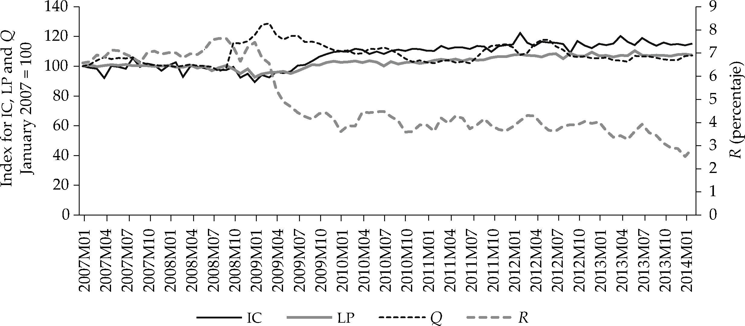
Figure 1 shows the behavior of ICt and a group of selected variables that, according to the battery of Granger causality tests presented in Section 6, display some prediction power over manufacturing international competitiveness (i.e., over ICt). First, it must be highlighted that our IC index fell from a peak of 105.6 units in August 2007 to a low of 89.4 units in January 2009. On the one hand, we must keep in mind that the US economic slowdown exerted a negative influence on US total manufacturing imports (M*t), thereby lowering external demand for Mexican manufactures. On the other hand, it appears that other significant forces were at play given that Mexican manufacturing exports to the US, Xt, declined somewhat faster than M*t. Among the many economic variables that could have had an important bearing on Xt, there are three that are measured on a monthly basis, display some prediction power over Xt, and report significant variation before or during the aforementioned period. Such three variables are: labor productivity, the real exchange rate and the real interest rate. First, according to Figure 1LP and IC follow the same pattern, given that both variables tend to fall before January 2009 and then basically tend to rise. Secondly, manufacturing IC deteriorates as the real interest rate increases (i.e., the inflation-adjusted interest rate on twenty-eight-day government bonds, CETES)3 and strengthens as the real interest rate goes down. Finally, by and large manufacturing IC and the real bilateral exchange rate exhibit a negative relationship, which is a counterintuitive point that will be further illustrated in Section 5.
, labor productivity (LP), real bilateral exchange rate (Q) and real interest rate (R) Source: author's estimations based on data from the US Census Bureau, the US Bureau of Labor Statistics and the National Institute of Statistics and Geography of México (Instituto Nacional de Estadística y Geografía, INEGI).")
Manufacturing international competitiveness (IC), labor productivity (LP), real bilateral exchange rate (Q) and real interest rate (R)
Source: author's estimations based on data from the US Census Bureau, the US Bureau of Labor Statistics and the National Institute of Statistics and Geography of México (Instituto Nacional de Estadística y Geografía, INEGI).
The IC index used here is intended to evaluate how fast Mexican manufacturing exports to the US are growing vis-à-vis US total manufacturing imports. In such a context, this paper relies to a great extent on the empirical literature regarding the shortand long-term determinants of exports. Broadly speaking, export equations are specified under the following four approaches: 1) gravity models of trade, 2) augmented gravity models of trade, 3) purely demand models, and 4) hybrid models combining demand and supply-side variables. Under the canonical form of the gravity model of trade, export volumes from one country to another are an increasing function of their economic sizes and a decreasing function of the transportation costs involved (Timbergen, 1962; Pöyhönen, 1963). Authors such as Bayoumi and Eichengreen (1997) and Bougheas, Demetriades and Morgenroth (1999) give rise to the augmented gravity model of trade by including other variables such as common language, shared borders and infrastructure. In a plausible attempt to further improve the explanatory power of the gravity trade equations, Soloaga and Winters (2001), Martínez-Zarzoso and Nowak-Lehmann (2002), and Rahman, Shadat and Das (2006) introduce new variables such as prices, exchange rates and exchange rate volatility, which are basically unrelated to space and geography.
A third strand of the literature is the one represented by traditional demand models, which posit the real exchange rate and the foreign income level as the two fundamental drivers of exports. Within this framework, many empirical studies conclude that exchange rate depreciation stimulates exports (and, therefore, IC) in developing countries through a favorable change in relative prices (Reinhart, 1995; Senhadji and Montenegro, 1999; Tellería, 2000; and Garcés, 2008). Nonetheless, the real exchange rate can also influence exports by changing relative unit labor costs as well as the local currency price of imported intermediate inputs, capital stock and technology.
Finally, there are many papers making use of both demandand supply-side variables to explain the dynamics of exports. Such an approach was originally motivated by Riedel (1998), who shows that neglecting supply-side variables in export demand equations leads to miss-specification problems and, therefore, biased estimates of export-demand elasticities. In this manner, this paper spurred the formulation of empirical models combining demand and supply-side variables, such as wages and labor productivity. In the case of developing economies, Catão and Falsetti (2002), Mbaye and Golub (2002) and Aysan and Hacihasanoglu (2007), inter alia, consider the impact of not only demandbut also supply-side variables, such as unit labor costs, on manufacturing exports. Broadly speaking, the evidence indicates that an increase in unit labor costs lowers manufacturing exports and vice versa. By decomposing unit labor costs’ movements into wage and productivity movements, Aysan and Hacihasanoglu (op. cit.) provide some evidence that a rise in productivity stimulates manufacturing exports whereas an increase in wages yields the opposite effect.
Along these lines, Feenstra, Li and Yu (2011) study the role of credit constraints in discouraging export volumes for a number of countries, concluding that the cost and availability of credit are key to exporting firms in need for short or long-term financing. Other authors find that FDI raises exports in developing economies, since host countries benefit from technology transfers and operate as a platform to export a wide variety of goods to advanced economies (Pacheco-López, 2005; Montobbio and Rampa, 2005). Furthermore, FDI is a major source of trade in intermediate inputs between parent and subsidiary companies, thereby increasing export volumes. In addition to FDI, there are many technology-related variables, such as research and development (R&D) expenditure and patenting activity, which influence export performance. In particular, Montobbio and Rampa (2005) and Menji (2010) draw attention to the link between technological factors and international trade.
THE MODEL AND THE DATAThis paper is concerned with estimating the impact of several key variables on Mexican manufacturing competitiveness in the US market, with the purpose of formulating policy recommendations. Although the choice of prospective explanatory variables is grounded on economic theory and previous econometric work, it is restricted by the availability of complete statistical series for the reference period (2007-2014). There are two concrete data limitations: First, the National Institute of Statistics and Geography of Mexico (Instituto Nacional de Estadística y Geografía, INEGI) broadened the coverage of the statistical data for the manufacturing sector from January 2007 on, with the aim of including the maquiladora exporting establishments. Therefore, the new data encompass a wider range of economic activity types and cannot be matched with the previous data to produce larger samples. Second, there is neither monthly nor quarterly data for key technology-related variables, such as research and development expenditure as a share of Gross Domestic Product (GDP) and the number of patents granted. Nevertheless, following Riedel's tradition (1998), it was possible to formulate a model comprising a reasonable number of demandand supply-side variables, together with a couple of control variables to deal with the so-called omitted variable bias.
A general-to-specific approach is utilized in the model building process, so that we depart from a large model and then perform a sequence of tests in order to attain a parsimonious and congruent final specification. Within this framework, we were able to produce an adjusted model which is theoretically plausible and stable, and whose residuals follow a multivariate normal white noise distribution. In principle, the next IC model is considered:

where: ICt is the international competitiveness index; Qt is the real bilateral exchange rate;4υt is the labor productivity in the manufacturing sector; Wt is the real average hourly wage in the manufacturing sector; Rt is the cost of credit as measured by the inflation-adjusted interest rate on twenty-eight-day government bonds (CETES); FDIt is the real Foreign Direct Investment in the manufacturing industry; CUt is the percentage capacity utilization in the manufacturing industry, and Lt is the occupied workers in the manufacturing industry.5
The next step was to collect monthly data for each variable from January 2007 to February 2014 (86 observations in all).6 The variables for which no compatible data are available prior to January 2007 are: labor productivity, υt, real wages, Wt, capacity utilization, CUt, occupied workers, Lt, and international competitiveness, ICt.7 There are other points that deserve special consideration: First, monthly data for FDI in the manufacturing sector are not available. Thus, in this particular case it was necessary to resort to quarterly data coupled with a frequency conversion method,8 which unfortunately entails an information loss. Second, all statistical series are seasonally adjusted by means of the X12-ARIMA procedure and, with the exception of Rt and CUt which are expressed in percentages, all the variables of the system are measured by indices and then stated in natural logarithms. Finally, both percentage CUt and Lt in the manufacturing industry have been included as control variables. These two control variables are helpful in dealing with potential under-specification problems (see, for instance, Athukorala and Suphachalasai, 2004; Berrettoni and Castresana, 2007), given the lack of monthly (or at least quarterly) data for many IC factors.
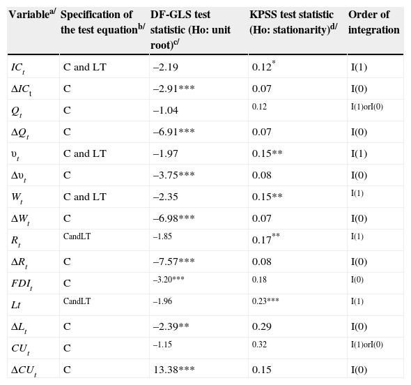
Integration analysisTo determine the order of integration of each variable, we make use of two types of standard tests: 1) Dickey-Fuller with Generalized Least Squares detrending (DF-GLS) developed by Elliott, Rothenberg and Stock (1996), which is the most powerful version of the unit root tests, and 2) Kwiatkowski, Phillips, Schmidt and Shin (KPSS, 1992), which is a stationarity test. As opposed to the unit root tests, the KPSS tests contrast the null hypothesis of stationarity against the alternative of unit root, and they are thus helpful in dealing with the lack of power of the unit root tests. To properly specify the test equations (that is, to determine whether to include a constant, a constant and a liner trend, or to omit both), the Hamilton methodology was used (Hamilton, 1994, p. 501). According to such a method, the specification of the test equation has to reflect the behavior of the time series not only under the unit root hypothesis, but also under the stationarity hypothesis. This method was enriched with a battery of F-type and t-type tests for the optional deterministic regressors, using the critical values developed by Dickey and Fuller (1981) and Dickey, Bell and Miller (1986) for that specific purpose.
As shown in Table 1, ICt seem to be integrated of order I (denoted I(1)) in levels and stationary in first differences. The same conclusion clearly applies to the following variables: υt, Wt, Rt, and Lt. In the case of Qt and CUt, unit root and stationarity tests produce conflicting results, which is certainly not uncommon. While the DF-GLS tests suggest that both variables are nonstationary, the KPSS tests lead to the opposite conclusion. In the specific case of Qt, the use of a larger time series (January 2000-February 2014) allow us to determine that this variable is in fact I(1) in levels. Nonetheless, in the case of CUt and other variables specifically linked to the manufacturing sector (such as υt, Wt and Lt) we have to deal with the limitation that the new data set starting January 2007 is not compatible with the old one. Therefore, the new and old data sets cannot be integrated to produce larger time series. In such a circumstance, to reach a sensible conclusion as to the order of integration of CUt, we make use of the old data set which provides a larger number of observations and apply the same tests. Using the period January 1994-December 2006 as a reference, it is possible to establish that CUt is I(1) in levels. Finally, the case of FDIt is to some extent atypical, given that this variable is subjected here to a frequency conversion procedure and turns out to be stationary (or I(0)). To fully validate this outcome, we take advantage of the fact that the Secretariat of Economy provides homogeneous quarterly data for FDIt since 1999. If we use quarterly data (i.e., if we omit the frequency conversion procedure) for the whole time interval (ranging from the first quarter of 1999 to the first quarter of 2014), the test results remain unchanged: FDIt is stationary variable. In summary, with the remarkable exception of FDIt which turns out to be stationary, all the variables of the model are I(1) in levels.
Mexican manufacturing industry: unit root and stationarity tests (January 2007-February 2014).
| Variablea/ | Specification of the test equationb/ | DF-GLS test statistic (Ho: unit root)c/ | KPSS test statistic (Ho: stationarity)d/ | Order of integration |
|---|---|---|---|---|
| ICt | C and LT | –2.19 | 0.12* | I(1) |
| ΔICt | C | –2.91*** | 0.07 | I(0) |
| Qt | C | –1.04 | 0.12 | I(1)orI(0) |
| ΔQt | C | –6.91*** | 0.07 | I(0) |
| υt | C and LT | –1.97 | 0.15** | I(1) |
| Δυt | C | –3.75*** | 0.08 | I(0) |
| Wt | C and LT | –2.35 | 0.15** | I(1) |
| ΔWt | C | –6.98*** | 0.07 | I(0) |
| Rt | CandLT | –1.85 | 0.17** | I(1) |
| ΔRt | C | –7.57*** | 0.08 | I(0) |
| FDIt | C | –3.20*** | 0.18 | I(0) |
| Lt | CandLT | –1.96 | 0.23*** | I(1) |
| ΔLt | C | –2.39** | 0.29 | I(0) |
| CUt | C | –1.15 | 0.32 | I(1)orI(0) |
| ΔCUt | C | 13.38*** | 0.15 | I(0) |
Notes:
* Rejection of Ho at the 10% significance level.
** Rejection of Ho at the 5% significance level.
*** Rejection of Ho at the 1% significance level.
a/ The symbol Δ is the first difference operator.
b/ C = Constant and LT = Linear Trend.
c/ The DF-GLS test results are based on the critical values developed by Elliott, Rothenberg and Stock (1996). The Schwarz Information Criterion is used to determine the lag length of each test equation.
d/ The KPSS test results are based on the critical values proposed by Kwiatkowski, Phillips, Schmidt and Shin (1992). To control the bandwidth, we use the Newey-West bandwidth selection method and the Bartlett Kernel.
Source: author's estimations based on monthly data from the INEGI, Mexico's Secretariat of Economy, the Foreign Trade Division of the US Census Bureau, and the US Bureau of Labor Statistics.
The time interval of this analysis, which comprises seven years, as well as the use of high-frequency (i.e., monthly) data make it difficult to conduct reliable co-integration analysis. Moreover, Johansen (1995) multivariate cointegration tests must depart from a congruent VAR model9 in levels, which is then reparameterised as a Vector Error-Correction (VEC) Model (Patterson, 2000, p. 615). While the first-difference (i.e., stationary) VAR model estimated in Section 5 exhibits fairly good statistical properties, the non-stationary VAR model used to test for cointegration displays signals of residual autocorrelation in spite of a series of remedial measures. Therefore, a plausible course of action is to differentiate the variables which are I(1), proceed to estimate a stationary VAR model and restrict the empirical analysis to the short-term horizon. A VAR model in first differences can be statistically acceptable whether the variables that includes (which are supposed to be I(1) in levels) are cointegrated or not (Patterson, 2000, p. 607).
A STATIONARY VAR MODELThis section deals with the estimation of a stationary VAR model. To arrive at a statistically appropriate final (or adjusted) specification, we estimate several alternative lag structures and information sets. The information set is given by the choice and number of variables of the system. In this regard, Patterson (2000, p. 164) points out that there may be a trade-off between the number of lags and the number variables included in the VAR. Equation [2] stands for the adjusted VAR model.

where Yt = [ΔICt,ΔQt,Δυt,ΔWt,ΔRt,ΔCUt,ΔLt]’ and represents a vector of endogenous variables. Moreover, Xt is a vector of exogenous regressors which includes a constant term and a couple of special effect dummy variables of the 0,1 form, which are useful to capture outliers and thus improve residual behavior. In particular, the dummy variables are introduced to capture the effects of the US subprime crisis on the variables of the model. Furthermore, ηt is a 7×1 vector of innovations, which are assumed to follow a multivariate normal white noise process. Such an assumption has the following constituent attributes: all the elements of ηt have zero-expected values and are homoscedastic, serially uncorrelated and normally distributed. Lastly, Bi (with i = 1, 2, 3, 4, 5) are the 7×7 coefficient matrices while Ω is a 7×3 coefficient matrix. As explained below, the model includes five lags for each variable in each equation.
It is also important to consider that E(ηt ηt) = Λ, where Λ is the covariance matrix of innovations of equation [2]. In principle, Λ is a non-diagonal matrix, so that VAR residuals are contemporaneously correlated and we are unable to link shocks to specific variables. To be able to refer to labor productivity shocks or real exchange rate shocks, it is necessary to eliminate the contemporaneous correlation among the constituent elements of innovation vector ηt. This critical task is fulfilled through the method developed by Pesaran and Shin (1998), which allows for the construction of an orthogonal set of innovations whose effects on the other variables of the system, do not rely on the VAR orderings. Recall that the main drawback of the traditional orthogonalization methodology proposed by Sims (1980) is that empirical results are sensitive to the order of the VAR equations.
The lag-length of the VAR model is crucial because it usually affects residual behavior as well as the empirical evidence. After exploring several lag structures and information sets, we reached the conclusion that five lags for each variable in each equation is an adequate choice for the VAR model on two grounds: First, it improves residual behavior. Second, it captures the dynamic adjustment of IC to shocks in the different variables of the system. As to the information set, it was found convenient to exclude FDI in the manufacturing industry from the model. The rational for doing so is twofold: On the one hand, including such variable gives rise not only to serial correlation in the VAR residuals, but also to severe deviations from normality. It is worth noting that changing the lag-length of the VAR models was ineffective in terms of lessening such problems. On the other hand, the dynamic response of IC to shocks in FDI systematically failed to reach statistical significance.
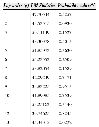
Model adequacy testingPrior to performing Granger-causality tests and estimating impulse-response functions, it is necessary to ascertain whether the stationary VAR model (i.e., Equation [2]) displays good statistical properties. In this manner, a battery of tests is conducted in order to show that our VAR model yields errors which are generally consistent with a multivariate normal white noise process. First of all, Table 2 depicts the outcome of the multivariate serial correlation Lagrange Multiplier (LM) tests. The LM statistics and their corresponding p-values indicate the absence of serial correlation up lag order thirteen. Put differently, we cannot reject the null hypothesis of no serial correlation up to lag order thirteen, at the 5 and 10 percent significance levels.
Mexican manufacturing industry: serial correlation Lagrange Multiplier (LM) tests for VAR residuals (January 2007-February 2014) Null hypothesis: there is no serial correlation at lag order (p).
| Lag order (p) | LM-Statistics | Probability valuesa/ |
|---|---|---|
| 1 | 47.70544 | 0.5257 |
| 2 | 43.53515 | 0.6936 |
| 3 | 59.11149 | 0.1527 |
| 4 | 48.30378 | 0.5013 |
| 5 | 51.85973 | 0.3630 |
| 6 | 55.23552 | 0.2509 |
| 7 | 58.82054 | 0.1589 |
| 8 | 42.09249 | 0.7471 |
| 9 | 33.83225 | 0.9513 |
| 10 | 41.89985 | 0.7539 |
| 11 | 53.25162 | 0.3140 |
| 12 | 39.74625 | 0.8245 |
| 13 | 45.34312 | 0.6222 |
Note: a/ Probability values stem from the Chi-Squared distribution with 49 degrees of freedom. Source: author's estimations based on monthly data from the INEGI, the Foreign Trade Division of the US Census Bureau, and the US Bureau of Labor Statistics.
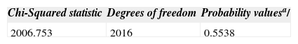
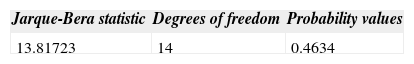
The multivariate version of the White heteroscedasticity test indicates that VAR residuals are homoscedastic. According to Table 3, the null hypothesis of homoscedasticity cannot be rejected and this result holds even at the 10% significance level. Furthermore, the Jarque-Bera normality test in Table 4 shows that VAR residuals are likely to follow a multivariate normal distribution, given that the probability value for the null hypothesis of residual multivariate normality is much larger than 10 percent.
Mexican manufacturing industry: White heroscedasticity tests for VAR residuals (January 2007-February 2014) Null hypothesis: homoscedasticity.
| Chi-Squared statistic | Degrees of freedom | Probability valuesa/ |
|---|---|---|
| 2006.753 | 2016 | 0.5538 |
Note: a/ Results correspond to the joint test with levels and squares only (no cross terms were included in the test equation).
Source: author's estimations based on monthly data from the INEGI, the Foreign Trade Division of the US Census Bureau, and the US Bureau of Labor Statistics.
Mexican manufacturing industry: Jarque-Bera normality test for VAR residuals (January 2007-February 2014)a/.
| Jarque-Bera statistic | Degrees of freedom | Probability values |
|---|---|---|
| 13.81723 | 14 | 0.4634 |
Note: a/ Results correspond to the joint test and VAR residuals are orthogonilized by the procedure developed by Lütkepohl (1991, pp. 155-158).
Source: author's estimations based on monthly data from the INEGI, the Foreign Trade Division of the US Census Bureau, and the US Bureau of Labor Statistics.
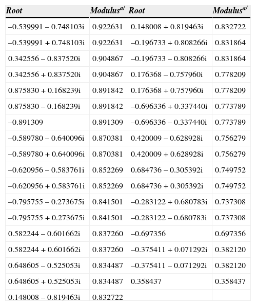
Finally, Table 5 shows that the VAR model is stable over time, given that all the inverse roots of the autoregressive characteristic polynomial lie within the unit circle (i.e., every root has modulus less than one).
Mexican manufacturing industry: Stability test based on the inverse roots of the autoregressive characteristic polynomial (January 2007-February 2014).
| Root | Modulusa/ | Root | Modulusa/ |
|---|---|---|---|
| –0.539991 – 0.748103i | 0.922631 | 0.148008 + 0.819463i | 0.832722 |
| –0.539991 + 0.748103i | 0.922631 | –0.196733 + 0.808266i | 0.831864 |
| 0.342556 – 0.837520i | 0.904867 | –0.196733 – 0.808266i | 0.831864 |
| 0.342556 + 0.837520i | 0.904867 | 0.176368 – 0.757960i | 0.778209 |
| 0.875830 + 0.168239i | 0.891842 | 0.176368 + 0.757960i | 0.778209 |
| 0.875830 – 0.168239i | 0.891842 | –0.696336 + 0.337440i | 0.773789 |
| –0.891309 | 0.891309 | –0.696336 – 0.337440i | 0.773789 |
| –0.589780 – 0.640096i | 0.870381 | 0.420009 – 0.628928i | 0.756279 |
| –0.589780 + 0.640096i | 0.870381 | 0.420009 + 0.628928i | 0.756279 |
| –0.620956 – 0.583761i | 0.852269 | 0.684736 – 0.305392i | 0.749752 |
| –0.620956 + 0.583761i | 0.852269 | 0.684736 + 0.305392i | 0.749752 |
| –0.795755 – 0.273675i | 0.841501 | –0.283122 + 0.680783i | 0.737308 |
| –0.795755 + 0.273675i | 0.841501 | –0.283122 – 0.680783i | 0.737308 |
| 0.582244 – 0.601662i | 0.837260 | –0.697356 | 0.697356 |
| 0.582244 + 0.601662i | 0.837260 | –0.375411 + 0.071292i | 0.382120 |
| 0.648605 – 0.525053i | 0.834487 | –0.375411 – 0.071292i | 0.382120 |
| 0.648605 + 0.525053i | 0.834487 | 0.358437 | 0.358437 |
| 0.148008 – 0.819463i | 0.832722 |
Note: a/ The stability condition is satisfied given that every root has modulus less than one.
Source: author's estimations based on monthly data from the INEGI, the Foreign Trade Division of the US Census Bureau, and the US Bureau of Labor Statistics.
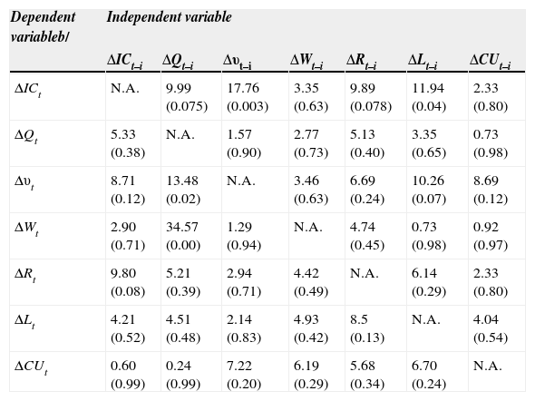
The next step is to carry out a battery of VAR-based Granger-causality tests, whose null hypothesis is that the coefficients of the lags of a particular variable are zero in a particular equation. The results of these tests are reported in Table 6 and the figures inside the parenthesis are significance levels. A significance level equal or smaller than 0.10 would allow one to reject the null hypothesis with a confidence level of at least 90%, which essentially means that the lags of the independent variable at issue are important in predicting the behavior of the dependent variable. In such a case, the implication is that the independent variable we are dealing with is a good predictor of the dependent variable.
Mexican manufacturing industry: VAR-based Granger-causality tests (January 2007-February 2014)a/ Null hypothesis: the coefficients of the lags of a given independent variable are zero in a particular equation.
| Dependent variableb/ | Independent variable | ||||||
|---|---|---|---|---|---|---|---|
| ΔICt–i | ΔQt–i | Δυt–i | ΔWt–i | ΔRt–i | ΔLt–i | ΔCUt–i | |
| ΔICt | N.A. | 9.99 (0.075) | 17.76 (0.003) | 3.35 (0.63) | 9.89 (0.078) | 11.94 (0.04) | 2.33 (0.80) |
| ΔQt | 5.33 (0.38) | N.A. | 1.57 (0.90) | 2.77 (0.73) | 5.13 (0.40) | 3.35 (0.65) | 0.73 (0.98) |
| Δυt | 8.71 (0.12) | 13.48 (0.02) | N.A. | 3.46 (0.63) | 6.69 (0.24) | 10.26 (0.07) | 8.69 (0.12) |
| ΔWt | 2.90 (0.71) | 34.57 (0.00) | 1.29 (0.94) | N.A. | 4.74 (0.45) | 0.73 (0.98) | 0.92 (0.97) |
| ΔRt | 9.80 (0.08) | 5.21 (0.39) | 2.94 (0.71) | 4.42 (0.49) | N.A. | 6.14 (0.29) | 2.33 (0.80) |
| ΔLt | 4.21 (0.52) | 4.51 (0.48) | 2.14 (0.83) | 4.93 (0.42) | 8.5 (0.13) | N.A. | 4.04 (0.54) |
| ΔCUt | 0.60 (0.99) | 0.24 (0.99) | 7.22 (0.20) | 6.19 (0.29) | 5.68 (0.34) | 6.70 (0.24) | N.A. |
Notes:
a/ The Granger-causality tests are based on χ2 —statistics with 5 degrees of freedom, given that the VAR model includes five lags. The numbers in parenthesis are significance levels.
b/ The symbol Δ is the first difference operator. Moreover, N.A. means Not Available in the standard testing procedure.
Source: author's estimations based on monthly data from the INEGI, the Foreign Trade Division of the US Census Bureau, and the US Bureau of Labor Statistics.
First, notice that the real exchange rate (ΔQt), labor productivity (Δυt), the real cost of credit (ΔRt) and occupied workers (ΔLt) have all some predictive power over ΔICt.10 At the same time, the evidence suggests that ΔICt have no predictive power over the real exchange rate, labor productivity and occupied workers, so that these three variables Granger-cause ΔICt. This finding is consistent with the view that improvements in productivity lead to higher exports and not the other way around (Wagner, 2007). On the other hand, there is a feedback system between ΔICt and ΔRt, given that ΔRt is a good predictor of ΔICt and vice versa. A plausible interpretation is that lower real interest rates encourage international competitiveness and exports but, eventually, higher exports and economic activity increase the private demand for credit and put pressure on real interest rates. Finally, it must be emphasized that the real exchange rate and occupied workers are good predictors of labor productivity, and that the real exchange rate is a good predictor of real wages.
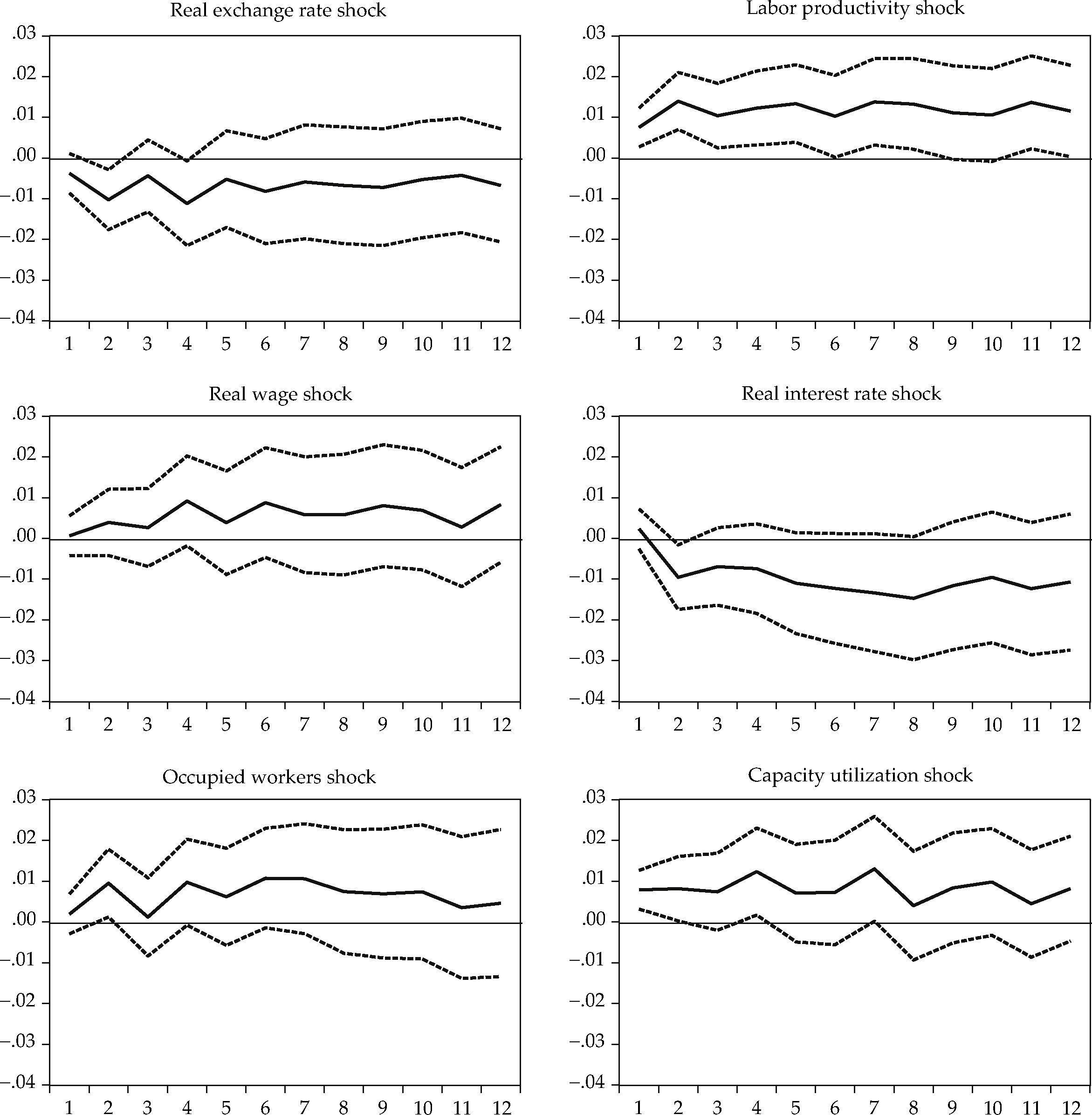
Generalized impulse-response functionsThe next step is to estimate a set of twelve-month impulse-response functions (IRF) with 95% confidence intervals. Figure 2 displays the IRF corresponding to our stationary VAR model (i.e., Equation [2]), which depicts the dynamic response of manufacturing IC to shocks in each variable of the system. Each shock, or innovation, must be thought of as a one-standard-deviation increase in the variable in question. Shocks are transitory as they last only one period (i.e., one month), whereas IRF are generalized in terms that they do not depend on the VAR orderings (Pesaran and Shin, 1998). On the other hand, the 95% confidence intervals are used to determine whether, and if so, to what extent IRF are statistically significant. Put differently, an IRF is statistically significant at the 5% level if and when its confidence interval leaves out the value zero. An important aspect to remember is that our VAR model is estimated in first differences. Therefore, the responses to shocks are not as noticeable as they would be, say, with a VAR model in levels. Nonetheless, most IRF achieve statistical significance at some point.
 Note: the dotted lines are 95% confidence intervals. Source: author's estimations based on montly data from INEGI, the Foreign Trade Division of the US Census Bureau, and the US Bureau of Labor Statistics.")
Mexican manufacturing sector. Dynamic response of international competitiveness to generalized schocks (January 2007-February 2014)
Note: the dotted lines are 95% confidence intervals.
Source: author's estimations based on montly data from INEGI, the Foreign Trade Division of the US Census Bureau, and the US Bureau of Labor Statistics.
The analysis of Figure 2 suggests that real exchange rate depreciation deteriorates (rather than strengthens) IC, at least in the short-term horizon. The negative effect of exchange rate depreciation on IC attains statistical significance around the second month and, before vanishing for good, regains some momentum around the fourth month. A labor productivity shock raises IC on impact and this positive influence is, to a certain degree, persistent over time. Real interest rate shocks have a short-lived (but nonetheless statistically significant) negative impact on IC, which takes place around the second month. Lastly, shocks to occupied workers raise IC around the second month while capacity utilization shocks enhance IC without delay but this effect fades away before the end of the second month. As part of the conclusions, we will see that these findings have important economic policy implications.
CONCLUSIONSThe empirical evidence supports three important conclusions, at least in the short-term horizon. First, real exchange rate depreciation reduces rather than increases IC in the short term. This is a counterintuitive finding, which is probably due to the fact that Mexico's exporting manufacturing sector depends to a large extent on imported intermediate inputs, capital stock and technology, so that real exchange rate depreciation influences IC through both demand and supply-side channels. On the demand side, it lowers the foreign-currency price of manufacturing exports, thereby strengthening IC. On the supply side, however, it increases the domestic-currency cost of imported intermediate inputs, capital goods and technology, thereby weakening IC. The net effect appears to be negative in the Mexican case (at least, in a short-term horizon), given the importance of cost competition and the sizable weight of the import content of manufacturing exports. A familiar policy prescription, which thus far has achieved very limited success, is to create and consolidate efficient production chains between large manufacturing firms and smalland medium-sized local enterprises, with a view to increasing the domestic content of manufactured products.
Secondly, a labor productivity increase significantly improves IC, which is consistent with the notion that Mexico's low investment in proper training programs represents an important obstacle to manufacturing IC. Although further research is required on the impact of labor productivity on IC, the evidence presented here supports the idea that the government should redouble its work with the private sector to design and implement a comprehensive, coherent and costeffective program to raise workers’ productivity in the manufacturing industry. Such a program must cover not only temporary training schemes to foster a given set of skills, but also continuous training arrangements aimed at mediumand long-term career development. In order for the training packages to emphasize the right knowledge, skills and abilities, the Mexican government, along with all the relevant interested parties (such as workers, employers, private sector training providers, and sector bodies), has to make an accurate identification and categorization of training requirements, not only for the overall manufacturing sector but also for every subsector and industry group. Given that technological change and innovation are continuously shaping employers’ demands, an adequate follow-up system must be launched to gather firsthand and reliable information on new training needs and future labor-market challenges.
Finally, the real interest rate is negatively related to IC, thereby suggesting that the high cost and relative unavailability of credit represent a burden to the Mexican manufacturing industry. This evidence highlights once again the role played by cost competition as well as the need to reduce the cost and legal requirements of shortand long-term financing. To that end, the recently approved financial reform in Mexico should at some point give manufacturing firms access to more competitive credit not only from development banks, but also from commercial banks. To describe such a reform or evaluate its possible impact is beyond the scope of this paper, but the conventional view is that its main two challenges have to do with the banking sector's oligopolistic structure (i.e., high market concentration and lack of competition) as well as the relative lack of rule of law institutions, devoted to solve problems between creditors and debtors. These two factors are, to a large extent, responsible for the persistently high financial intermediation costs that prevail in the Mexican economy.
In January 2007, the National Institute of Statistics and Geography of Mexico (Instituto Nacional de Estadística y Geografía, INEGI) broadened the coverage of the statistical data regarding the manufacturing sector, in order to include the maquiladora exporting establishments. Therefore, from this date on, the standard manufacturing data cover 240 types of economic activity according to the North American Industrial Classification System (NAICS) 2007.
Source: own estimation based on data from the INEGI and the International Trade Administration database of the US Department of Commerce.
The interest rate on twenty-eight-day government bonds works as a reference rate, given that many debt instruments, such as commercial papers and bank acceptances, fix their rates in the open market accordingly. However, it is taken only as a proxy for the cost of credit since many manufacturing exporting firms get subsidized loans from Banco Nacional de Comercio Exterior and some others resort to commercial bank loans, whose interest rates are not known on a monthly basis.
The real bilateral exchange rate was calculated in the standard fashion: Qt = eP*/P, where e is the peso-dollar nominal exchange rate, P* the US price level, and P is the Mexican price level.
According to the INEGI, an occupied worker is the one who worked at least one hour a week during the reference period.
Source: INEGI, Mexico's Secretariat of Economy, the Foreign Trade Division of the US Census Bureau, and the US Bureau of Labor Statistics.