


The present paper analyzes the effects of ECB monetary policy on the Spanish stock market returns. The data sample run all over the euro period: from January 1999 to December 2014. This period is split into two well-defined sub-periods based on the structural change brought about by the financial crisis in August 2007. Spanish stock market returns are approximated by the returns of the selective index Ibex 35 while monetary policy of the Eurozone is measured by the nominal target interest rate on the last day of the month. With regard to the methodology, as I am interested in the long-term relationship between the two variables aforementioned, a structural vector autoregressive (SVAR) model. The results show that monetary policy shocks have a considerable effect on the Spanish stock market returns in the long run. The results also show that monetary policy shocks of the ECB monetary policy lead to a different long-term effect in the pre-crisis period and the post-crisis sample.
As is well known, European Central Bank (ECB) monetary policy authorities can influence stock market returns via different channels, such as the interest rate channel, the credit channel, the asset price channel, the exchange rate channel and the expectations channel (ECB, 2010). One of these channels, the asset price channel, based on the Ando and Modigliani (1963) and Tobin's q (1969) theories, is the focus of the present paper. The great number of changes in financial markets that have changed the existing framework of both the international and national financial fields (Rajan, 2006) and the form in how financial transactions are made, and thus in assuming risk, have led monetary policy decision-makers to analyze how their measures affect financial markets in this new environment. Furthermore, recent research (Gambacorta, 2009; Bekaert et al., 2013; Nave and Ruiz, 2015) suggests that benign economic environments might promote excessive risk taking and might actually make the financial system more fragile. Therefore, since the financial crisis began in mid-2007, monetary policy may have promoted financial markets instability (Altunbas et al., 2010; Gambacorta and Marques-Ibanez, 2011; Mishkin, 2011).
In this context, this study is designed to analyze the relationship between monetary policy and stock prices of the Spanish equity market before and after the financial crisis started. This focus is why the monetary policy of reference is led by the ECB and why the period of analysis is limited to the beginning of the third phase of the Economic and Monetary Union in January 1999. However, in the spirit of Patelis (1997), who found that increases in the federal funds rate have a significant negative impact on predicted stock returns in the short run, but a positive one at longer horizons, I am interested not only in the contemporaneous relation between monetary policy and stock prices, but also in the cumulative long-term effect of monetary policy on stock prices.
Among the usual methodologies applied in this context, a structural VAR approach is adopted as in Crowder (2006), since it is the only method that fits with the research goal. Alternative methodologies as the event study methodology (Bredin et al., 2007; Fiordelisi et al., 2014) and the heteroskedasticity approach (Rigobon, 2003; Rigobon and Sack, 2004; Bohl et al., 2008) are only appropriate to analyze the behavior of stock prices around the monetary policy interventions. Certainly, the short-run market response can be suggestive of policies’ long-term effectiveness (Ait-Sahalia et al., 2012), but only that. On the other hand, methodologies based on regression analysis (Angeloni and Ehrmann, 2003; Napolitano, 2009) do not avoid endogeneity problems between monetary policy shocks and stock prices. Instead, the structural VAR is a popular approach among macroeconomists to analyze whether monetary shocks have real effects avoiding endogeneity problems among variables, and the inclusion of asset prices in such models along with other proxies of the underlying economy would be useful in settling the issue of measuring the specific long-term effects of monetary policy on financial markets.
The literature that assesses the impact of monetary policy on stock prices is mainly focused on U.S. markets (Patelis, 1997; Thorbecke, 1997; Bomfim, 2003; Ehrmann and Fratzscher, 2004; Rigobon and Sack, 2004; Bernanke and Kuttner, 2005; Gürkaynak et al., 2005; Crowder, 2006; Davig and Gerlach, 2006; Chen, 2007; Bjørnland and Leitemo, 2009; Chuliá et al., 2010; Rangel, 2011; Rosa, 2011; Galí and Gambetti, 2014) with the exceptions of Fiordelisi et al. (2014) that measure a “global” effect, and Angeloni and Ehrmann (2003), Bohl et al. (2008), Napolitano (2009), and Bredin et al. (2009) that are focused on European markets. We can also find several papers that analyze the impact of monetary policy shocks in stock market centered in particular countries, as Bredin et al. (2007) and Gregoriou et al. (2009) for the UK, Vithessonthi and Techarongrojwong (2012) for Thailand, Jain et al. (2011) for Australia, Duran et al. (2012) for Turkey and Koivu (2012) for China, among others.
However, none of the papers that included the ECB policy and Eurozone markets is aimed to analyze the cumulative long-term effect of monetary policy shocks on stock prices. On the other hand, only the works by Fiordelisi et al. (2014) and Galí and Gambetti (2014) deal with the financial crisis period, although those are not related specifically to the ECB policy and Eurozone markets, but are focusing on the short-run market response. Moreover, as their analysis is limited to the financial crisis period, they cannot measure the differences, if any, of the monetary policy effects on stock prices due to the economic turmoil.
Previous studies in an international finance context (Andersen et al., 2007; Ammer and Wongswan, 2007; Craine and Martin, 2008; Albuquerque and Vega, 2009) suggest that national equity markets are positively correlated to macroeconomic global factors. Others (Wongswan, 2006; Ammer et al., 2010; Laeven and Tong, 2012; Jinjarak, 2013) used the Fed monetary policy stance as a global macroeconomic factor or examined the effect of Fed monetary policy shocks on foreign equity indexes. To take into account this global factor is the reason why I also include the US monetary policy in the analysis.
Thus, to the best of my knowledge, this paper contributes to the previous literature in two ways: It is the first one focused on measuring the cumulative long-term effect of the ECB monetary policy shocks on Spanish stock prices; secondly, it is the first one focused on measuring differences on that effect, if any, due to the recent financial crisis.
The remainder of this paper is structured as follows: Section 2 gives a short introduction to the methodology used. Section 3 describes the factors, variables and data used in the analysis. Section 4 presents the main results. Finally, in Section 5 the conclusions are summarized.
2MethodologyA SVAR model is a system of simultaneous equations that allows us to analyze interactions among the variables that compose the model, where the contemporary values of the variables appear as explicative variables in different unrestricted equations. That is, the same group of explicative variables appear in each of the equations. Each variable, being all considered endogenous, is then explained by its own lagged values and by the current and past values for the rest of the variables in the system. The VAR model is a generally accepted way to analyze relationships within a group of variables and is used extensively in the literature on monetary policy, where shocks in this policy are interpreted as represented by the shocks in the monetary policy equation included in the model.
In the SVAR model I consider five endogenous factors presented in the next section are considered, that is, the direction of ECB monetary policy (ecbmp), the Spanish stock market return (spsr), the European business cycle (eubc), the domestic inflation as target in the domestic monetary policy (inf), and the direction of FED monetary policy (fedmp) to control for the effects of US monetary policy on the other factors considered (Rigobon, 2003; Nave and Ruiz, 2015). These factors are collected using vector Xt=(fedmpt,;eubct,inft,ecbmpt,spsrt).
Without losing generality, we can consider the following structural VAR without constants:
where A is a matrix containing the parameters of contemporary relationships between the endogenous variables of the model; Xt−1 is a matrix of the endogenous variables lagged for one period; Φ is a matrix of the model parameters; and ¿t is the vector of structural shocks, i.e., the components of the endogenous variable that are not explained by the model.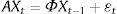
To estimate the above SVAR model I must formulate it as a reduced VAR and rewrite (1) in the following way:
where B is A−1Φ, and C is A−1.
To correctly identify the structural relationship, I must add restrictions in the SVAR; to do this the Cholesky decomposition of the estimation of the covariant variances matrix is used. This decomposition places restrictions on matrix A, which gathers contemporary relationships. Now the order of variables becomes especially relevant because depending on their position within vector X the variable values are to be explained by the contemporary values of the other variables or not.
We can order variables taking into account both the economic logic confirmed by empirical evidence and the final objective of the analysis. Namely, I allow that the Spanish stock market return responds instantaneously to FED and ECB monetary policy shocks. The direction of ECB monetary policy also responds instantaneously to the direction of FED monetary policy without the same happening in reverse, although in this case, this restriction would have little importance given the objective of this study.
3Factors, variables, sample and dataThe period of analysis considered in this study begins in January 1999, the date when the Euro was introduced along with the common monetary policy run by the ECB (Fahr et al., 2013), and ends in December 2014. Thus, the whole sample covers 192 observations of monthly data. The period includes two well-defined sub-periods based on the well-known structural change brought about by the financial crisis in August 2007. The pre-crisis sub-period sample covers the first 103 monthly observations, and the post-crisis (start) sub-period sample covers the following 89 months.
The five factors involved in the analyses are: (i) the stance of the domestic monetary authority policy; (ii) the domestic inflation as target in the domestic monetary policy; (iii) the Spanish stock market return; (iv) the business cycle in the domestic currency area; and (v) a global monetary policy factor. The five factors included in the SVAR model are measured as follows.
To measure the domestic business cycle I use one of the several proxies usually employed in literature. Specifically, to proxy Eurozone business cycle variations, I employ the monthly growth rate of the Eurozone industrial production index (IPI). Later, to analyze the robustness of our results, I replace this rate by the Eurozone unemployment rate at the end of the month and the Eurozone monthly growth rate of the gross domestic product (GDP). Domestic monetary policy is measured by the stance of the domestic monetary authority, through the nominal target interest rate on the last day of the month set by the monetary authority, the ECB in the Eurozone case. The domestic inflation rate is measured as the monthly inter-annual variation rate of the CPI. For the Eurozone I use the harmonized consumer price index (HICP). Finally, the Spanish stock market return is computed using data of the benchmark stock market index IBEX35. I use the last day of the month data to compute monthly continuous compounding returns.
The model is enlarged to include a fifth variable as a proxy of the global monetary policy factor: the Fed monetary policy shocks. To measure the Fed monetary policy shocks I use the residuals of the monetary policy stance equation in the four-factor SVAR base model estimated with data from the US dollar area. This auxiliary model is formed by the four domestic factors described above but referred to the US dollar area. The US stock market return is computed using data of the benchmark stock market index S&P500. The monetary policy of the Fed is measured using the target interest rate on the last day of the month. The US inflation rate is measured as the US consumer price index (US-CPI) inter-annual variation rate. The US business cycle is measured by US industrial production index (US-IPI) inter-annual growth rate.
4Results4.1Four variables SVAR. Results for a local modelThe analysis begins with a four variables model: (i) the stance of the domestic monetary authority policy; (ii) the domestic inflation as target in the domestic monetary policy; (iii) the Spanish stock market return (spsr) (iv) the business cycle in the domestic currency area.
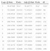
4.2Results for the pre-crisis sampleTo select the correct VAR order I use the Akaike (AIC), Hannan-Quinn (HQIC), and the Schwarz Bayesian (SBIC) information criteria and also the final prediction error (FPE) and the likelihood ratio (LR) statistic. Results are shown in Table 1. The optimal lag is one in SBIC and HQIC, so I use a model with one lag. As reflected in Table 2, the specified model is stable, indicated by the fact that all the auto values are below one, and thus stationary. Moreover, the Portmanteau test, shown in Table 3 shows that the self-correlation is not completely removed.
Selection of the optimal lag in the 4-variable SVAR. The variables used in this analysis are IPI growth rate, Eurozone HCPI, Eurozone interest rate and IBEX35 return. The period of the sample covers January 1999 until July 2007. The following criteria were used in this analysis: LR: sequentially modified LR test statistic; FPE: final prediction error; AIC: Akaike information criterion; SC: Schwarz information criterion; and HQ: Hannan-Quinn information criterion. 99-07.
| Lags | LR | FPE | AIC | SC | HQ |
|---|---|---|---|---|---|
| 0 | NA | 0.156307 | 9.495574 | 9.603106 | 9.539025 |
| 1 | 537.0350 | 0.000561 | 3.865361 | 4.403019* | 4.082615* |
| 2 | 31.15424 | 0.000548 | 3.839944 | 4.807729 | 4.231002 |
| 3 | 35.81423 | 0.000498 | 3.740028 | 5.137939 | 4.304889 |
| 4 | 28.32357 | 0.000489 | 3.713747 | 5.541785 | 4.452412 |
| 5 | 23.47069 | 0.000506 | 3.733418 | 5.991582 | 4.645886 |
| 6 | 20.36113 | 0.000541 | 3.779386 | 6.467678 | 4.865658 |
| 7 | 29.45932 | 0.000500 | 3.669875 | 6.788293 | 4.929950 |
| 8 | 27.58315* | 0.000467* | 3.561828* | 7.110372 | 4.995706 |
The symbol * indicates the optimal lag order selected for each criterion.
Analysis of the stability of the 4-variable pre-crisis SVAR. In this analysis, the roots of the characteristic VAR polynomial are determined as defined by the IPI, HCPI, ECB interest rate, IBEX35 variables and specified for 1 lag. The model is stable if all the roots are lower than 1. In this case, the VAR satisfied the condition of stability.
| Root | Modulus |
|---|---|
| 0.920738−0.054393i | 0.922343 |
| 0.920738+0.054393i | 0.922343 |
| 0.837360 | 0.837360 |
| −0.124204 | 0.124204 |
No root lies outside the unit circle.
VAR satisfies the stability condition.
Autocorrelation analysis of the residuals of the pre-crisis SVAR. A Portmanteau test was conducted to confirm the self-correlation of the residuals up to lag 12. This result contrasts to the null hypothesis of absent self-correlation until this lag. This period became established because monthly frequency data were used.
| Lags | Q-Stat. | Prob. | Adj. Q-Stat. | Prob. | df |
|---|---|---|---|---|---|
| 1 | 21.96972 | NA* | 22.18724 | NA* | NA* |
| 2 | 37.75409 | 0.1279 | 38.28730 | 0.1161 | 29 |
| 3 | 62.91486 | 0.0399 | 64.21052 | 0.0314 | 45 |
| 4 | 83.42121 | 0.0299 | 85.55386 | 0.0208 | 61 |
| 5 | 118.3985 | 0.0017 | 122.3341 | 0.0008 | 77 |
| 6 | 146.0816 | 0.0004 | 151.7474 | 0.0001 | 93 |
| 7 | 173.6482 | 0.0001 | 181.3452 | 0.0000 | 109 |
| 8 | 189.3414 | 0.0002 | 198.3741 | 0.0000 | 125 |
| 9 | 210.1312 | 0.0001 | 221.1757 | 0.0000 | 141 |
| 10 | 229.2823 | 0.0001 | 242.4084 | 0.0000 | 157 |
| 11 | 245.9900 | 0.0002 | 261.1358 | 0.0000 | 173 |
| 12 | 277.2740 | 0.0000 | 296.5910 | 0.0000 | 189 |
The symbol * indicates the test is valid only for lags larger than the VAR lag order.
The results in terms of impulse-response functions (IRF) for the estimated SVAR with exclusion restrictions on the contemporary responses described above are shown in Fig. 1. All the IRF include confidence intervals to 68%, commonly used in calculated VAR analyses, and computed using bootstrap techniques with 1000 replications. Shocks, as usual, have been normalized to a standard deviation of the variable that provides the impulse.
.")
Impulse-response functions for a 4-variable SVAR. Pre-crisis sample. The entire analysis contained in this figure across its 2 panels uses the variables of IPI growth rate, HCPI, ECB interest rate and IBEX35 return. For all of the figures, confidence intervals of 68% calculated using a bootstrap with 1000 replications (Fisher and Hall, 1991).
Thus, a monetary shock equaling a reduction of the nominal interest rate of 15.12 basis points, as we can see in Fig. 1 Panel A, has a positive and significant (at 68%) effect on the stock market return from the first month until seventeen months later, with a maximum value of 4.33 b.p., in the first period, and a cumulative and significant response from the sixth month until the end of the period considered, reaching a maximum value of 45.99 basis points as Fig. 1 Panel B shows.
4.3Results for the post-crisis sampleNow, as we can see in Table 4, the optimal lag is one in SBIC, so I implement a SVAR model with 1 lag. As Table 5 shows, the specified model is stable, i.e., stationary. However, Table 6 shows self-correlation in some residuals until lag 12.
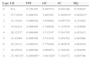
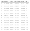
Selection of the optimal lag in the post-crisis SVAR. The period of the sample covers from August 2007 to December 2014. The following criteria were used in this analysis: LR: sequentially modified LR test statistic; FPE: final prediction error; AIC: Akaike information criterion; SC: Schwarz information criterion; and HQ: Hannan-Quinn information criterion.
| Lags | LR | FPE | AIC | SC | HQ |
|---|---|---|---|---|---|
| 0 | NA | 6.787620 | 13.26660 | 13.40267 | 13.32012 |
| 1 | 493.8709 | 0.002264 | 5.259519 | 5.939879* | 5.527108 |
| 2 | 52.76480* | 0.001425* | 4.790330* | 6.014978 | 5.271990* |
| 3 | 12.63444 | 0.001870 | 5.045577 | 6.814514 | 5.741309 |
| 4 | 18.62564 | 0.002138 | 5.148609 | 7.461834 | 6.058411 |
| 5 | 15.09053 | 0.002610 | 5.297247 | 8.154760 | 6.421121 |
| 6 | 19.49110 | 0.002809 | 5.292260 | 8.694061 | 6.630205 |
| 7 | 14.75505 | 0.003393 | 5.366224 | 9.312314 | 6.918241 |
| 8 | 11.30228 | 0.004553 | 5.497418 | 9.987796 | 7.263506 |
The symbol * indicates the optimal lag order selected for each criterion.
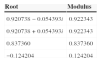
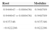
Analysis of the stability of the 4-variable SVAR for the post-crisis period. In this analysis, the roots of the characteristic VAR polynomial are determined as defined by the variables considered and specified for 1 lag. The model is stable if all the roots are lower than 1. In this case, the VAR satisfied the condition of stability.
| Root | Modulus |
|---|---|
| 0.944643−0.086436i | 0.948589 |
| 0.944643+0.086436i | 0.948589 |
| 0.935346 | 0.935346 |
| −0.022286 | 0.022286 |
Autocorrelation analysis of the residuals of the post-crisis SVAR. A Portmanteau test was conducted to confirm the self-correlation of the residuals up to lag 12. This result contrasts to the null hypothesis of absent self-correlation until this lag. This period became established because monthly frequency data were used.
| Lags | Q-Stat. | Prob. | Adj. Q-Stat. | Prob. | df |
|---|---|---|---|---|---|
| 1 | 41.46366 | NA* | 41.96322 | NA* | NA* |
| 2 | 62.19145 | 0.0003 | 63.19657 | 0.0002 | 29 |
| 3 | 85.88696 | 0.0002 | 87.76968 | 0.0001 | 45 |
| 4 | 100.2831 | 0.0011 | 102.8856 | 0.0006 | 61 |
| 5 | 117.8709 | 0.0019 | 121.5866 | 0.0009 | 77 |
| 6 | 130.0227 | 0.0068 | 134.6731 | 0.0031 | 93 |
| 7 | 141.5349 | 0.0197 | 147.2319 | 0.0086 | 109 |
| 8 | 159.2568 | 0.0208 | 166.8193 | 0.0074 | 125 |
| 9 | 176.9744 | 0.0216 | 186.6629 | 0.0060 | 141 |
| 10 | 196.6580 | 0.0174 | 209.0065 | 0.0035 | 157 |
| 11 | 220.0867 | 0.0090 | 235.9655 | 0.0010 | 173 |
| 12 | 251.9977 | 0.0015 | 273.1951 | 0.0001 | 189 |
The symbol * indicates the test is valid only for lags larger than the VAR lag order.
The results in terms of impulse-response functions (IRF) for the estimated SVAR are shown in Fig. 2. In this case, a monetary shock equaling a reduction of the nominal interest rate of 13.52 basis points, as we can see in Fig. 2 Panel A, has an effect on the stock market return positive and significant (at 68%) from 4 months after up to 10 months after, accumulating a no significant response as Fig. 2 Panel B shows.
4.4Five variables SVAR. Results for a global model
The model is broadened to include as fifth variable a proxy of the global monetary policy factor: the Fed monetary policy shocks. To measure the Fed monetary policy shocks I use the residuals of the monetary policy stance equation in the four-factor SVAR base model estimated with data from the US dollar area. This analysis helps to understand whether the results regarding the effects of domestic monetary policy on Spanish stock market returns change when I add the global monetary policy factor in the enlarged model.
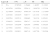
4.5Pre-crisis sampleFirst of all, the correct VAR order is selected, as we can see in Table 7, the optimal lag is one in SBIC, HQIC and FPE. As reflected in Table 8, the specified model is stable, and the Portmanteau test, shown in Table 9 shows that the self-correlation is not completely remove.
Selection of the optimal lag in the 5 variables SVAR. Pre-crisis. The period of the sample covers from January 1999 to July 2007. The following criteria were used in this analysis: LR: sequentially modified LR test statistic; FPE: final prediction error; AIC: Akaike information criterion; SC: Schwarz information criterion; and HQ: Hannan-Quinn information criterion.
| Lags | LR | FPE | AIC | SC | HQ |
|---|---|---|---|---|---|
| 0 | NA | 0.002695 | 8.272993 | 8.407407 | 8.327306 |
| 1 | 532.6859 | 1.15e−05* | 2.814073 | 3.620560* | 3.139954* |
| 2 | 33.88898 | 1.30e−05 | 2.936949 | 4.415509 | 3.534398 |
| 3 | 50.92952 | 1.17e−05 | 2.818587 | 4.969220 | 3.687604 |
| 4 | 30.72781 | 1.34e−05 | 2.929662 | 5.752368 | 4.070247 |
| 5 | 31.89431 | 1.48e−05 | 2.993741 | 6.488520 | 4.405894 |
| 6 | 26.59133 | 1.74e−05 | 3.104568 | 7.271419 | 4.788288 |
| 7 | 39.72508 | 1.62e−05 | 2.957577 | 7.796502 | 4.912866 |
| 8 | 37.87353* | 1.50e−05 | 2.782531* | 8.293529 | 5.009387 |
The symbol * indicates the optimal lag order selected for each criterion.
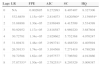
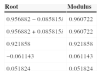
Analysis of the stability of the 5-variable SVAR for the pre-crisis sample. The VAR is specified for 1 lag. In this case, the VAR satisfied the condition of stability.
| Root | Modulus |
|---|---|
| 0.905555−0.031753i | 0.906111 |
| 0.905555+0.031753i | 0.906111 |
| 0.839812 | 0.839812 |
| −0.115713−0.074064i | 0.137386 |
| −0.115713+0.074064i | 0.137386 |
Autocorrelation analysis of the residuals of the pre-crisis sample for the 5 variables SVAR. A Portmanteau test was conducted to confirm the self-correlation of the residuals up to lag 12.
| Lags | Q-Stat. | Prob. | Adj. Q-Stat. | Prob. | df |
|---|---|---|---|---|---|
| 1 | 24.16937 | NA* | 24.40867 | NA* | NA* |
| 2 | 46.31548 | 0.4592 | 46.99770 | 0.4314 | 46 |
| 3 | 83.53357 | 0.1467 | 85.34361 | 0.1178 | 71 |
| 4 | 109.6776 | 0.1608 | 112.5547 | 0.1191 | 96 |
| 5 | 151.2008 | 0.0327 | 156.2183 | 0.0171 | 121 |
| 6 | 184.7638 | 0.0165 | 191.8790 | 0.0065 | 146 |
| 7 | 230.3409 | 0.0017 | 240.8144 | 0.0003 | 171 |
| 8 | 252.2278 | 0.0042 | 264.5641 | 0.0008 | 196 |
| 9 | 282.1631 | 0.0034 | 297.3963 | 0.0005 | 221 |
| 10 | 313.9261 | 0.0022 | 332.6118 | 0.0002 | 246 |
| 11 | 340.5247 | 0.0026 | 362.4256 | 0.0002 | 271 |
| 12 | 377.2921 | 0.0010 | 404.0954 | 0.0000 | 296 |
The symbol * indicates the test is valid only for lags larger than the VAR lag order.
The results in terms of impulse-response functions for the estimated SVAR are shown in Fig. 3. Panel A. Thus, a monetary shock equaling a reduction of the nominal interest rate of 14.9 basis points, has a positive and significant (at 68%) effect on the stock market return from the first month until sixteen months later, with a maximum value of 4.45 b.p., in the first period. We can also observe a significant contemporaneous negative response equaling −9.67 b.p.
, in which the sample period runs from January 1999 to July 2007.")
When we observe the cumulative response we can notice a significant increase of 68% and has a cumulative value of 40.83 b.p. from the seventh month until the end of the period considered, as Fig. 3 Panel B shows.
4.6Post-crisis sampleWhen I analyze the post-crisis sample for the 5 SVAR model, we can see in Table 10, the optimal lag is one in SBIC and HQIC, so I implement a SVAR model with 1 lag. As Table 11 shows, the specified model is stable, i.e., stationary. However, Table 12 shows self-correlation in some residuals until lag 12.
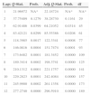
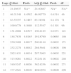
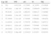
Selection of the optimal lag in the 5 variables SVAR. Post-crisis. The period of the sample covers from August 2007 to December 2014.
| Lag | LR | FPE | AIC | SC | HQ |
|---|---|---|---|---|---|
| 0 | NA | 0.073356 | 11.57695 | 11.72476 | 11.63626 |
| 1 | 685.5941 | 1.46e−05 | 3.052983 | 3.939816* | 3.408792* |
| 2 | 56.42101 | 1.22e−05 | 2.864252 | 4.490113 | 3.516569 |
| 3 | 29.89995 | 1.45e−05 | 3.021537 | 5.386425 | 3.970361 |
| 4 | 55.33649 | 1.11e−05 | 2.716546 | 5.820462 | 3.961878 |
| 5 | 31.82058 | 1.22e−05 | 2.755274 | 6.598217 | 4.297113 |
| 6 | 20.88211 | 1.62e−05 | 2.954916 | 7.536886 | 4.793263 |
| 7 | 46.67498 | 1.21e−05 | 2.534978 | 7.855976 | 4.669832 |
| 8 | 41.79322* | 9.46e−06* | 2.107432* | 8.167457 | 4.538793 |
The symbol * indicates the optimal lag order selected for each criterion.
Autocorrelation analysis of the residuals of the post-crisis sample for the 5 variables SVAR. A Portmanteau test was conducted to confirm the self-correlation of the residuals up to lag 12.
| Lags | Q-Stat. | Prob. | Adj. Q-Stat. | Prob. | df |
|---|---|---|---|---|---|
| 1 | 36.07309 | NA* | 36.48773 | NA* | NA* |
| 2 | 70.24480 | 0.0122 | 71.45412 | 0.0095 | 46 |
| 3 | 109.9510 | 0.0021 | 112.5617 | 0.0012 | 71 |
| 4 | 149.2505 | 0.0004 | 153.7326 | 0.0002 | 96 |
| 5 | 168.7016 | 0.0027 | 174.3555 | 0.0011 | 121 |
| 6 | 189.4750 | 0.0090 | 196.6489 | 0.0033 | 146 |
| 7 | 208.4985 | 0.0267 | 217.3164 | 0.0095 | 171 |
| 8 | 246.1622 | 0.0087 | 258.7465 | 0.0018 | 196 |
| 9 | 286.2860 | 0.0020 | 303.4413 | 0.0002 | 221 |
| 10 | 320.3295 | 0.0010 | 341.8494 | 0.0001 | 246 |
| 11 | 351.6174 | 0.0007 | 377.6069 | 0.0000 | 271 |
| 12 | 400.9305 | 0.0000 | 434.7064 | 0.0000 | 296 |
The symbol * indicates the test is valid only for lags larger than the VAR lag order.
The results in terms of impulse-response functions (IRF) for the estimated SVAR are shown in Fig. 4. In this case, a monetary shock equaling a reduction of the nominal interest rate of 13.64 basis points, as we can notice in Fig. 4 Panel A, has an effect on the stock market return positive and significant (at 68%) from 4 months after up to 10 months after, accumulating a no significant response as Fig. 4 Panel B shows.
4.7Robustness analysis
The analysis in each sample was repeated using different variables as ECB monetary policy measure: concretely, the growth rate of the M1 monetary mass, the real interest rates of the ECB, as difference between nominal interest rate and inflation rate, and deviations according to Taylor's Rule. All the results corroborate those formerly obtained. The analysis was also repeated replacing the economic cycle measure used, the Eurozone IPI growth rate, with the Eurozone unemployment rate and with the GDP growth rate of the Eurozone. Once again, all the results corroborate the effects found earlier.
5ConclusionsIn the introduction of this paper two questions are posed thus far unanswered: What is the long-run effect of ECB monetary policy on the Spanish stock market returns? and Has that effect changed in the recent financial crisis period? To answer these two questions, an analysis by using the structural VAR approach with four variables has been performed: the two entities directly involved in the questions (i.e., the ECB monetary policy and the Spanish stock market returns); and another two variables that contribute to define the ECB monetary policy shocks, that is, the European business cycle and the domestic inflation as target in the domestic monetary policy. Later the model has been broadened to include as fifth variable a proxy of the global monetary policy factor: the Fed monetary policy shocks.
The results show that monetary policy shocks have a considerable effect on the Spanish stock market returns in the long run for the pre-crisis period. Accordingly, a reduction of the nominal interest rate has a positive and significant accumulative effect on the Spanish stock market return from the sixth month until the end of the period considered. When I analyze the post-crisis period the monetary policy has no significant effect on the Spanish stock market returns in the long run.
This result remains constant when I control with a global factor, the US monetary policy. In this case, during the pre-crisis period, a monetary policy shock has a positive and accumulative significant effect on the Spanish stock market returns, in the long run, fewer and shorter than when is not taking into account this global effect. When I analyze the post-crisis period the effect of the monetary policy would remain no significant in the long run.
These results show the inability of monetary authorities, in the post-crisis period, to perform conventional measures based on managing official interest rates when they are close to zero levels and the need to implement unconventional measures of monetary policy in the euro area.
The author thanks comments from Gonzalo Rubio, María Asunción Prats, Marta Regúlez, David Toscano, Ricardo Gimeno and Mariano González. The author is also grateful for comments from participants in the 77th International Atlantic Economic Conference (Madrid – Spain, 2014) and in the XXIII Finance Forum (Madrid – Spain, 2015) in particular to Kristle Cortés, and the anonymous reviewer and the editors of the SRFE. Finally, I especially thank the great support and comments from Juan Nave.

