


Because of the noises from the internal and external factors, the uncertainty increases in the financial market. The challenges of nonlinearities, volatility clusters, and multiple structural breaks which entail risk. Due to the risk, the prediction task becomes more complex. First, this work proposes a hybrid model to predict the one-day future price for the stocks; MSFT, Apple, Goldman Sachs and JP Morgan use the Markov switching model coupled with radial basis function network for prediction. Second, this paper forecasts the buy/sell trading strategy using the proposed hybrid method. Also, this paper explores the risk of investment decisions and the trading performance based on different value at risk (VaR) methods. Finally, by comparing the proposed model results with the pure linear and non-linear models, the prediction efficiency is evaluated. The experimental results indicate the investment risk, and the investment trading strategy provides a better accuracy with the best investment decision for the selected stocks.
Structural break, volatility modelling, and forecasting problems are considered as important tasks in the financial time series applications. This paper introduces a novel hybrid architecture called Markov switching Autoregressive model (4) combined with Bayesian Regularized Radial Basis Function Neural Network MSAR (4) (BR-RBFN) as a forecaster. Recently, researchers are attracted towards the pole of the stock price trend prediction which is embodied an increasing development in the model building process for evaluating the better investment stocks in the trading business. These models provide an investment trading insight to the investors who are forging the business deals in the trading market. Now, this profit maximization model demands an efficient market situation where investors are expected to yield a higher profit. However, if the market is efficient, it is not always easy to anticipate an investor who can yield a maximum profit than those who are holding the random stocks (Malkiel, 2003). So, it is vital to evaluate the unit root test with the presence of multiple structural changes for efficient market hypothesis.
Naturally, the impulses (structural changes, conflicting behaviour, and political policy changes) from the internal and the external factors are predominantly changing the price direction. Thus, these deterministic changes and inherent noises make the prediction task even more complicated. The cornerstone of the prediction is that if the stock returns are mean revert, it will be possible to forecast the future trend using the past information data, as given in Malkiel and Fama (1970). There are a number of studies dealing with the efficient market hypothesis by examining the random walk analysis using different unit root tests for the emerging market (Gough and Malik, 2005; Lim and Brooks, 2011; Mishra et al., 2015; Borges, 2010). However, very few studies have allowed the structural changes in the unit root test for improving the prediction performance of the considered model. A study in the US on monthly natural gas consumption with the presence of GARCH unit root test and structural breaks has suggested that there is strong evidence of stationarity in the data, as mentioned by Mishra and Smyth (2014). Using macroeconomic time series data, a comparative analysis of structural break has been analyzed for improving the prediction performance (Bauwens et al., 2015). Based on the mathematical Bai-Perron technique, the housing price of the United States has been predicted by the presence of multiple structural breaks (Barari et al., 2014).
A number of studies have been analyzed for understanding the importance of parametric and non-parametric models, which are used in the application of time series forecasting. In finance, stock return prediction of Intraday S&P 500 index has been evaluated to improve the prediction accuracy as discussed in Matías and Reboredo (2012). This study suggests that the non-linear models surpassed the traditional linear models such as random walk on the basis of both statistical and economic criteria. In order to estimate and fine-tune the parameters of the non- linear STAR model, an evolutionary programming based on genetic algorithm has been utilized for forecasting the Eurozone peripheral stock market provided in Avdoulas et al. (2015). This study discusses the important implication of the market efficacy and predictability in terms of the investment trading strategies.
In recent years, Artificial Neural Networks play a major role in predicting the stock price trends (Ghiassi et al., 2005; Roh, 2007; Hamzaçebi et al., 2009; Patel et al., 2015). Oil price forecasts have been reviewed using the following price forecasting techniques such as ANN, genetic algorithm, support vector machine and hybrid system, which have been elaborated in Sehgal and Pandey (2015). Thereafter, a number of advanced mathematical techniques including fuzzy logic, genetic algorithm, and Bayesian probability have been exploited to improve the stock price trend prediction (Atsalakis and Valavanis, 2009; Chen et al., 2007; Chang, 2012; Ticknor, 2013; Sun et al., 2014; Ariyo et al., 2014). To perceive the plague of overfitting and overtraining of the neural network and to improve the network generalization, many hybridized studies have been developed for stock price trend prediction (Babu and Reddy, 2014; Adhikari and Agrawal, 2014). For predicting the electricity price, a hybrid ANN model has been proposed by Chaâbane (2014). The potential benefits and impact of accurate stock market prediction of Taiwan Stock Exchange Capitalization Weighted Stock Index (TAIEX), Dow-Jones Industrial Average (DIA), S&P 500 and IBOVESPA Stock Index have been investigated by Chen and Chen (2015). Similarly, a combination of genetic algorithm with support vector machine has been modified to uncover the short-term trading efficiency of ASE 20 Index, which has been evaluated by Karathanasopoulos et al. (2015). Although there are many potential linear and non-linear stock price trend prediction models available in the academic literature, it is worthy of mention that no single model is best in all situations (Zhang, 2004).
First, this paper proposes a novel architecture in order to improve the strength of each non-linear model such as Markov switching model and radial basis function network model to predict the one-day future stock price for the four major stock returns. Then, this proposed model finds its predictive ability and improves the network generalization, as well as overcoming the plague of network overfitting and overtraining. Though there are a number of studies available on risk modelling, the single model reliability is still questionable. To the best of our knowledge, the combination of two non-parametric models has not yet contributed to the burgeoning literature for predicting the future stock returns.
Second, this study predicts the buy/sell trading days for the considered stock returns to improve the trading performance using the hybrid optimal cost function. Also, this paper investigates the investment decision peril based on the value at risk forecasts (VaR) using the parametric methods such as MA, EWMA, GARCH, historical simulation and expected shortfall. Finally, by comparing the proposed model results with the traditional Random walk linear model (RW) and the non-linear models such as Smooth transition autoregressive model (STAR), Multilayer Perceptron network (MLP), and Random forest network, the prediction efficiency is evaluated.
The rest of the paper is structured as follows. Section 2 describes the methodology of the proposed hybrid model; Sections 3 and 3.1 consider the data and the technical indicators and their importance; Section 4 discusses empirical analysis; Section 4.1 confers the results of the predictive hybrid model; finally, Section 5 summarizes the conclusions of this study.
2Methodology2.1Markov switching modelA non-linear threshold Markov switching model has potentially been employed to estimate the multiple structural changes and to predict the one-day future diurnal stock return patterns. The effects of structural shocks are characterized over two-regimes in the parameter estimation. During the model building process, this model's flexibility allows the different types of behavioural patterns for the considered stock returns at different points in time. Hence, it helps to capture the multiple structural changes in the data and provides useful signal about the market activities.
Basically, Markov switching model by Hamilton (1996) implies that the probability distribution of an unobserved variable yt lying in the interval {a, b} depends on their state at the time t−1 and not on any previous states.
Let us consider the unobserved state variable be St. Now the series of each considered stock data can be represented as follows:
where εt∼N(0,1). In state 1, the expected returns and the error variances are represented as (μ,σ2). Similarly, in state 2, they are (μ0+μ,σ2+θ). The unknown parameters μ0, μ, σ02, σ2, p11, p22 can be estimated using maximum likelihood method. An easily computable technique called the Hamilton filter gives statistically significant values for the unknown parameters based on its means.2.2Bayesian regularized radial basis function network


In 1988, Broomhead and Lowe exploited the use of radial-basis functions in the design of the neural network. The radial basis function network is a three-layered architecture labelled as the input layer, a hidden layer, and the output layer (Broomhead and Lowe, 1988) as illustrated in Fig. 1. The input layer consists of 10 nodes of input neurons Xi. The hidden layer consists of the same number of evaluation units as the size of the training sample N; each unit is mathematically described by a radial basis function F that has the following structure:
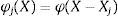
where {φ(X−Xi)|i=1,2,…,N} is a set of non-linear function known as radial-basis functions and ||.|| denotes a norm. The known data points Xi∈ℝm0, i=1,2,…,N are considered to be the centres of the radial-basis functions. Basically, high-dimensional space leads to the problem of the multivariable interpolation problem (Davis, 1963). Therefore, this interpolation problem can be stated as follows: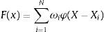


Now, the simultaneous linear equation for the unknown coefficients of expansion {wi} are given by
The N×1 vector d and ω represent the desired response vector and linear weight vector, respectively. ϕ denotes a N×N matrix with the elements φij.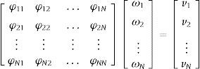

The interpolation matrix is represented as
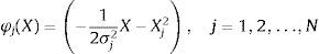
The weight vector in the hidden layer can be solved byHenceforth, each computational unit in the hidden layer of the network that can be evaluated using the Gaussian function is defined bywhere σj is a measure of the width of the jth Gaussian function with the centre Xj.

The output layer consists of a single computational linear unit. Typically, the size of the output layer is much smaller than that of the hidden layer. For network training, the Bayesian regularized method has been utilized to estimate the optimum network parameters such as spread and weights. Thus, the optimized network's parameters provide better prediction accuracy and improve the network generalization by removing the plague of network overfitting and overtraining. This method adds the error term in the optimal cost function as follows:
where yt is optimal cost function; ES is sum of squared errors of the considered stock returns; Ew is sum of square of network weights; and u and v are the cost function parameters.
Using the Bayes’ rule, the density function can be represented as follows:
where w is network weight; S is considered stock data; and M is network model.
By solving Hessian matrix of yt, the optimal function converges to its minimum point at wminimum point. The regularized parameters u and v are evaluated using the Gauss-Newton approximation method given in Foresee and Hagan (1997).
2.3Hybrid predictive methodIn this study, two widely popular non-linear models, Markov switching AR (4) and Radial Basis Function network model, are exploited to predict the one-day future stock returns. First, this idea was proposed by Zhang (2004), and was further revised and explored by Khashei and Bijari (2011). From their studies, it is observed that the aggregate of two single models can efficiently improve the forecast accuracy of the considered stock return data than any single linear and nonlinear models do.
The proposed hybrid model is considered as a function of two non-linear components.
Thus,
where yt represents each stock return observations at time t. N1t and N2t are the non-linear components of Markov switching AR (4) model and radial basis function network model, respectively. Now,

This proposed method consists of the following three steps. First, the Markov switching AR (4) model has successfully captured the multiple structural changes and has effectively estimated the model parameters for the given stock returns. Such a model produces a series of predictions defined as N1t. Hence, the obtained residual is denoted as et containing the non-linear patterns in the considered time series data, which can be represented as follows:
where N1t is the predicted values of the Markov switching model at time 1t. ¿t is represented as the noise in the time series. Second, the radial basis function network model is utilized to explore the non-linear patterns of the obtained residuals, which are labelled as N2t. Finally, the predictions of Markov switching AR (4) component (N1t) and the radial basis function network component (N2t) are recombined to generate an aggregate prediction.

Thus, the estimated aggregate prediction is represented as below:

Hence, this proposed hybrid method is not only improving the strength of single nonlinear model's prediction accuracy, but also is expunging the issues of skewness and the serial correlation of the considered stock returns. Also, this method would overcome the plaque of network overfitting and overtraining using the probabilistic regularization method. This feature of the network randomly assigns weights to the network parameter, which is efficiently improving the network generalization. The proposed model framework is shown in Fig. 2.
3Data BR-RBFN framework.")
For empirical analysis, four major stocks, Microsoft (MSFT), Apple Inc. (Apple), Goldman Sachs (GMS) and JP Morgan Chase &Co (JPM), are selected to predict the one-day future stock price returns using the proposed hybrid model. The total number of samples for the considered stocks are 1257 daily trading days, from 3 January 2011 to 31 December 2015 including open, high, low, close price, trading volumes, and foremost seven technical indicators. From Fig. 1, it is shown that the four considered stock price returns exhibit different patterns in the upward direction, and provide the importance of trends to the investors or the traders so that they can make investment decisions based on the buy/sell trading strategy. The first 80% of the samples have been chosen as training set while the remaining 20% of the samples comprised of the testing set. In model building process, the training set is used to estimate the model parameters by increasing the number of hidden layer neurons until the parameters reached to its constant value and the testing set is used to select an appropriate model for forecasting the stock returns.
In this study, a comparative analysis is also conducted to test the network performance of the proposed model efficacy, with the pure traditional linear and some of the widely used nonlinear models such as Random walk, MSAR (4), STAR, MLP, BR-RBFN, and Random forest (Fig. 3).
3.1Technical Indicators
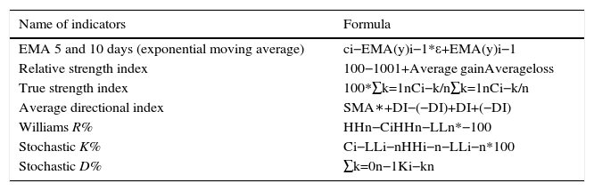
Seven technical indicators were employed as a portion of the input variables to the network. It is often utilized by the investors who seem to predict the future price trend of an asset by looking at its past trend pattern. In the existing literature, it is vital to deduce the major indicators to make decisions in the investment trade market, as presented in Kara et al. (2011). These indicators are calculated using their formulae from the considered raw stock data. Indicators and their respective formulae are summarized in Table 1.
Selected technical indicators.
| Name of indicators | Formula |
|---|---|
| EMA 5 and 10 days (exponential moving average) | ci−EMA(y)i−1*ε+EMA(y)i−1 |
| Relative strength index | 100−1001+Average gainAverageloss |
| True strength index | 100*∑k=1nCi−k/n∑k=1nCi−k/n |
| Average directional index | SMA∗+DI−(−DI)+DI+(−DI) |
| Williams R% | HHn−CiHHn−LLn*−100 |
| Stochastic K% | Ci−LLi−nHHi−n−LLi−n*100 |
| Stochastic D% | ∑k=0n−1Ki−kn |
Ci is the closing price, ¿=2/(1+y), y is the time period for 5 or 10 days moving average, HHn is the highest high, LLD is the lowest low in past n days, DI=+DM/TR; −DI=−DM/TR, +DM=Wilders exponential moving average of +DM; −DM=Wilders exponential moving average of −DM; TR=Wilders exponential moving average of TR.
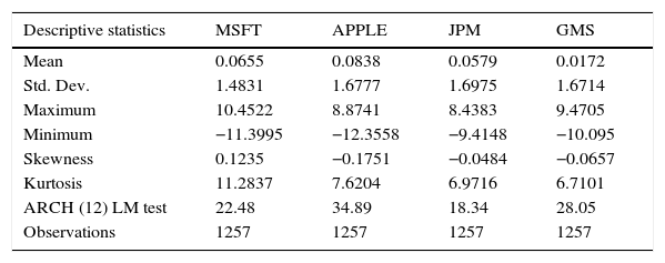
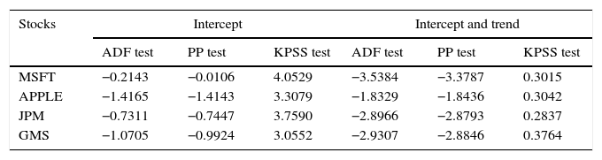
The summary statistics for daily considered stock returns from 2011 to 2015 is presented in Table 2. The daily mean for all the stock returns is small while the volatility of Apple, JPM and GMS are around 1.7% and the volatility of MSFT is around 1.5%. Further, the mean grows at a linear rate while volatility grows approximately at a square root rate. As seen over the time period, the expected return dominates the risk. The returns of Apple, JPM, and GMS have a very small negative skewness, which implies that the probability of the occurrence of negative daily returns is higher on the considered stock returns with a high kurtosis. Finally, the ARCH-LM test shows that there is a significant time-varying volatility presence in the daily stock returns by rejecting the null hypothesis of no arch effect at 5 percent level for all the given stocks. For exploring the unit-root in the given series, the traditional unit root tests with and without trend have been performed using the ADF (Augmented Dickey-Fuller), the PP (Phillips-Perron) and KPSS (Kwiatkowski, Phillips, Schmidt, and Shin). The results are presented in Table 3. The stocks MSFT, Apple, GMS, and JPM confirm the presence of a unit root in the time series – meaning that in all the cases, the statistical values are fallen into the region of rejection at 1%, 5% and 10% significance level.
Descriptive statistics of the considered stock returns yt.
| Descriptive statistics | MSFT | APPLE | JPM | GMS |
|---|---|---|---|---|
| Mean | 0.0655 | 0.0838 | 0.0579 | 0.0172 |
| Std. Dev. | 1.4831 | 1.6777 | 1.6975 | 1.6714 |
| Maximum | 10.4522 | 8.8741 | 8.4383 | 9.4705 |
| Minimum | −11.3995 | −12.3558 | −9.4148 | −10.095 |
| Skewness | 0.1235 | −0.1751 | −0.0484 | −0.0657 |
| Kurtosis | 11.2837 | 7.6204 | 6.9716 | 6.7101 |
| ARCH (12) LM test | 22.48 | 34.89 | 18.34 | 28.05 |
| Observations | 1257 | 1257 | 1257 | 1257 |
Results of traditional unit root test.
| Stocks | Intercept | Intercept and trend | ||||
|---|---|---|---|---|---|---|
| ADF test | PP test | KPSS test | ADF test | PP test | KPSS test | |
| MSFT | −0.2143 | −0.0106 | 4.0529 | −3.5384 | −3.3787 | 0.3015 |
| APPLE | −1.4165 | −1.4143 | 3.3079 | −1.8329 | −1.8436 | 0.3042 |
| JPM | −0.7311 | −0.7447 | 3.7590 | −2.8966 | −2.8793 | 0.2837 |
| GMS | −1.0705 | −0.9924 | 3.0552 | −2.9307 | −2.8846 | 0.3764 |
Note: Significance at levels 5%.
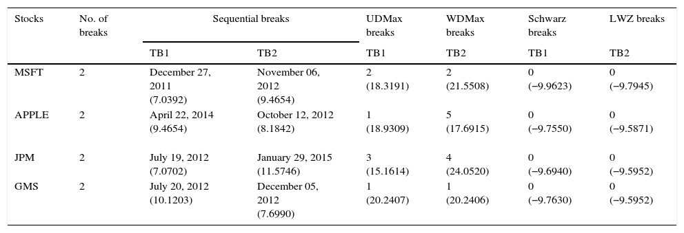
The results for the multiple-break Bai and Perron (2003) unit root test are presented in Table 4. The multiple structural changes have been identified by Bai and Perron test statistics. It efficiently captures the maximum number of breaks vˆ(TBˆ) (maximum number of allowing breaks are Five) using the HAC estimator kˆT for the given stock returns. The function supFT(l+1|l) with 15% trimming value has been sequentially utilized to estimate the structural changes at 5% significance level. It is found that the stocks MSFT, Apple, JPM, and GMS contain two structural breaks during the sequential process of multiple structural changes over the given time period. The major breaks have been identified in the years 2011, 2012, and 2015 over the given period. Therefore, the sequential test statistic FT(2|1),FT(3|2) for the given stocks is found to be (7.0392, 9.4654), (9.4654, 8.1842), (7.0702, 11.5746), and (10.1203, 7.6990). Similarly, for another test statistics UDMax,WDMax, values of MSFT, Apple, JPM, and GMS are (18.3191, 21.5508), (18.9309, 17.6915), (15.1614, 24.0520), and (20.2407, 20.2406), respectively. Finally, LWE criteria and Schwarz criteria significantly locate the breaks at the 5% level.
Results for multiple structural changes by Bai and Perron test (2003).
| Stocks | No. of breaks | Sequential breaks | UDMax breaks | WDMax breaks | Schwarz breaks | LWZ breaks | |
|---|---|---|---|---|---|---|---|
| TB1 | TB2 | TB1 | TB2 | TB1 | TB2 | ||
| MSFT | 2 | December 27, 2011 (7.0392) | November 06, 2012 (9.4654) | 2 (18.3191) | 2 (21.5508) | 0 (−9.9623) | 0 (−9.7945) |
| APPLE | 2 | April 22, 2014 (9.4654) | October 12, 2012 (8.1842) | 1 (18.9309) | 5 (17.6915) | 0 (−9.7550) | 0 (−9.5871) |
| JPM | 2 | July 19, 2012 (7.0702) | January 29, 2015 (11.5746) | 3 (15.1614) | 4 (24.0520) | 0 (−9.6940) | 0 (−9.5952) |
| GMS | 2 | July 20, 2012 (10.1203) | December 05, 2012 (7.6990) | 1 (20.2407) | 1 (20.2406) | 0 (−9.7630) | 0 (−9.5952) |
Note: The values in brackets are value of structural break statistic compared with the Bai-Perron critical values (2003).
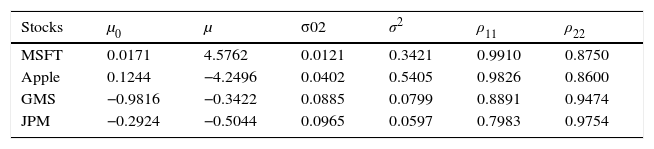
The multiple structural changes of the considered stock returns have been successfully modelled by Markov switching AR (4) model. The estimated parameters of Markov switching AR (4) model are presented in Table 5. The estimated returns (means) and risks (variances) for each stock data have been varied in the given two regimes. It is shown that the prices of MSFT and Apple stock returns are relatively higher than the stock returns of GMS and JPM. Also, each stock return is persistent for the shorter period than the longer time period. Naturally, the multiple structural changes cause the problem of poor prediction performance of the model. Thus, this Markov switching AR (4) model does not give any guarantee that it is the best single, reliable model for forecasting in every situation.
The results of Markov switching AR (4) model.
| Stocks | μ0 | μ | σ02 | σ2 | ρ11 | ρ22 |
|---|---|---|---|---|---|---|
| MSFT | 0.0171 | 4.5762 | 0.0121 | 0.3421 | 0.9910 | 0.8750 |
| Apple | 0.1244 | −4.2496 | 0.0402 | 0.5405 | 0.9826 | 0.8600 |
| GMS | −0.9816 | −0.3422 | 0.0885 | 0.0799 | 0.8891 | 0.9474 |
| JPM | −0.2924 | −0.5044 | 0.0965 | 0.0597 | 0.7983 | 0.9754 |
Note:(μ0,μ) – estimated means of regime 1 and 2; (σ02,σ2) – estimated variances of regime 1 and 2; ρ11 – probability of being in regime one; ρ22 – probability of being in regime two.
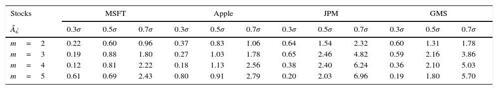
Next, the obtained residuals from the selected Markov switching AR (4) model is presented in Table 6. The residual's non-linear pattern has been identified by the BDS test, which suggests that the null hypothesis of i.i.d has fallen in the rejected region at 5% significance level, as given in Broock et al. (1996). Thus, there is clear evidence of the non-linear structure that exists in the residual data for the considered stock returns. To enhance the proposed model predictive performance, this non-linear residual structure is necessary to be fed into the neural network system to build a better model.
BDS test results on residuals from Markov switching AR (4) model.
| Stocks | MSFT | Apple | JPM | GMS | ||||||||
|---|---|---|---|---|---|---|---|---|---|---|---|---|
| ¿ | 0.3σ | 0.5σ | 0.7σ | 0.3σ | 0.5σ | 0.7σ | 0.3σ | 0.5σ | 0.7σ | 0.3σ | 0.5σ | 0.7σ |
| m=2 | 0.22 | 0.60 | 0.96 | 0.37 | 0.83 | 1.06 | 0.64 | 1.54 | 2.32 | 0.60 | 1.31 | 1.78 |
| m=3 | 0.19 | 0.88 | 1.80 | 0.27 | 1.03 | 1.78 | 0.65 | 2.46 | 4.82 | 0.59 | 2.16 | 3.86 |
| m=4 | 0.12 | 0.81 | 2.22 | 0.18 | 1.13 | 2.56 | 0.38 | 2.40 | 6.24 | 0.36 | 2.10 | 5.03 |
| m=5 | 0.61 | 0.69 | 2.43 | 0.80 | 0.91 | 2.79 | 0.20 | 2.03 | 6.96 | 0.19 | 1.80 | 5.70 |
Note: ¿ – the distance between the measure of standard deviations from the raw data; σ – standard deviations; m – embedding dimension.
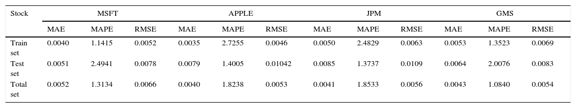
Table 7 shows the simulated results of the stocks MSFT, Apple, GMS, and JPM. The Mean Absolute Error (MAE), Mean Absolute Percentage Error (MAPE), and Root Mean Square Error (RMSE) are evaluated for the training, testing and the total data set to perceive the proposed model effectiveness of the given stock returns. With the lowest error measures, the proposed MSAR (4) BR-RBFN model can provide a good prediction value for the one-day future stock return, which is greater than 98.5% precision.
Forecast accuracy of hybrid Markov switching AR (4) BR-RBFN model.
| Stock | MSFT | APPLE | JPM | GMS | ||||||||
|---|---|---|---|---|---|---|---|---|---|---|---|---|
| MAE | MAPE | RMSE | MAE | MAPE | RMSE | MAE | MAPE | RMSE | MAE | MAPE | RMSE | |
| Train set | 0.0040 | 1.1415 | 0.0052 | 0.0035 | 2.7255 | 0.0046 | 0.0050 | 2.4829 | 0.0063 | 0.0053 | 1.3523 | 0.0069 |
| Test set | 0.0051 | 2.4941 | 0.0078 | 0.0079 | 1.4005 | 0.01042 | 0.0085 | 1.3737 | 0.0109 | 0.0064 | 2.0076 | 0.0083 |
| Total set | 0.0052 | 1.3134 | 0.0066 | 0.0040 | 1.8238 | 0.0053 | 0.0041 | 1.8533 | 0.0056 | 0.0043 | 1.0840 | 0.0054 |
Note: Significance level at 5%.
The simulated results of the proposed model for all the considered stocks are shown in Fig. 4(a)–(d). It is noticed that the actual values are not deviating much from its predicted value – meaning that the difference between the observed values and the predicted values are relatively small. Similarly, Fig. 5(a)–(d) shows the linear fitness curve of the stock returns MSFT and JPM. This study exploits a large number of data for testing the proposed model generalization with the presence of significant noises and structural changes. It is observed that the dotted line indicates the perfect fitness with slope one. The values spreading around the dotted line are the minimum error values of the actual and the predicted values. Thus, testing data provides the evidence of an appropriate model generalization and robustness with the reduced error values.
–(d) The predicting results of the MSFT, Apple, GMS, and JPM total data set.")

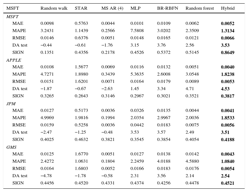
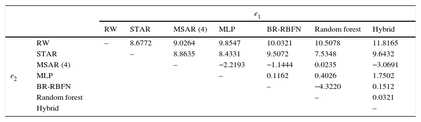
In order to explore the proposed model prediction accuracy, the error measures (MAE, MAPE, RMSE and proportion of the signs of return) are properly evaluated. The directional prediction changes for one-step ahead forecast are calculated using the DA test given in Pesaran and Timmermann (1992). As presented in Table 8, the goodness of fit for the pure linear and non-linear models is investigated by the statistical error values, based on one-step ahead forecasting values. The conclusions are twofold. First, the results of MSFT, APPLE, JPM, and GMS are heterogeneous based on the log-likelihood estimation, in terms of error measures and DA test measure. The MSAR (4) model tends to be the best nonlinear model in terms of MAE and RMSE error values. It is rarely outperformed by other non-linear models such as STAR, MLP, BR-RBFN and Random forest for one-day ahead prediction. As for MAPE error values, the hybrid model results are outperforming the linear and other nonlinear models for all the considered stock returns at the near future period. Taking into account the proportion of Sign test, BR-RBFN model performs well than other models for the considered stock returns. The DA test of the null hypothesis of actual and predicted values is independent at 5% significance level for Random Walk, STAR, and MSAR (4) models that are rejected at the given time period. However, the MLP, BR-RBFN, Random forest, and Hybrid models do not reject the null hypothesis at any significance level. DA forecast accuracy is always providing a better indication of the investment trading strategy of the stock returns. Second, DM forecast accuracy test for RMSE examines whether the two models are statistically significant. Table 9 shows the forecast errors on e1 and e2, which is shown in the upper triangular matrix. The lower triangular matrix is omitted because of the matrix symmetry. Now, the linear Random walk model is compared with all other non-linear models and vice versa. Then, the smaller RMSE values indicate the traditional linear model which naturally performs worse than other STAR, MSAR (4), BR-RBFN, Random forest and the proposed hybrid model. Despite all other nonlinear models being able to improve the forecast accuracy, the null hypothesis of true forecast errors for the considered stocks, which are identically zero, is not always constantly rejected. From the overall comparison, the results of nonlinear models show the hybrid MSAR (4) Br-RBFN model, which performs better than the linear and other nonlinear models such as STAR, MSAR (4), MLP, BR-RBFN, and Random forest in terms of the goodness of fit.
Comparison of hybrid model forecast accuracy with the traditional linear and nonlinear models for the considered stocks.
| MSFT | Random walk | STAR | MS AR (4) | MLP | BR-RBFN | Random forest | Hybrid |
|---|---|---|---|---|---|---|---|
| MSFT | |||||||
| MAE | 0.0098 | 0.5763 | 0.0044 | 0.0101 | 0.0109 | 0.0062 | 0.0052 |
| MAPE | 3.2431 | 1.1439 | 0.2566 | 7.5808 | 3.0202 | 2.3509 | 1.3134 |
| RMSE | 0.0146 | 0.6376 | 0.0051 | 0.0148 | 0.0165 | 0.0121 | 0.0066 |
| DA test | −0.44 | −0.61 | −1.76 | 3.15 | 3.76 | 2.56 | 3.53 |
| SIGN | 0.1351 | 0.4356 | 0.2178 | 0.4526 | 0.5372 | 0.5145 | 0.8649 |
| APPLE | |||||||
| MAE | 0.0108 | 1.5677 | 0.0069 | 0.0116 | 0.0132 | 0.0051 | 0.0040 |
| MAPE | 4.7271 | 1.8980 | 0.3439 | 5.3635 | 2.6008 | 3.0548 | 1.8238 |
| RMSE | 0.0151 | 1.6201 | 0.0071 | 0.0164 | 0.0179 | 0.0089 | 0.0053 |
| DA test | −1.87 | −0.67 | −2.63 | 1.45 | 3.34 | 4.71 | 4.53 |
| SIGN | 0.3265 | 0.2643 | 0.3146 | 0.2967 | 0.3021 | 0.3521 | 0.3817 |
| JPM | |||||||
| MAE | 0.0127 | 0.5173 | 0.0036 | 0.0326 | 0.0135 | 0.0044 | 0.0041 |
| MAPE | 4.9969 | 1.9816 | 0.1994 | 2.0354 | 2.9967 | 2.0036 | 1.8533 |
| RMSE | 0.0159 | 0.5258 | 0.0036 | 0.0442 | 0.0183 | 0.0075 | 0.0056 |
| DA test | −2.47 | −1.25 | −0.48 | 3.53 | 3.57 | 2.49 | 3.51 |
| SIGN | 0.4025 | 0.4632 | 0.3821 | 0.3545 | 0.3854 | 0.4054 | 0.4188 |
| GMS | |||||||
| MAE | 0.0125 | 1.6770 | 0.0051 | 0.0127 | 0.0138 | 0.0142 | 0.0043 |
| MAPE | 2.4272 | 1.0631 | 0.1804 | 2.2459 | 4.0188 | 4.5880 | 1.0840 |
| RMSE | 0.0164 | 1.6803 | 0.0052 | 0.0166 | 0.0183 | 0.0176 | 0.0054 |
| DA test | −4.78 | −1.78 | −0.58 | 2.31 | 3.56 | 2.14 | 2.54 |
| SIGN | 0.4456 | 0.4520 | 0.4331 | 0.4374 | 0.4256 | 0.4478 | 0.4521 |
Note: Significance level at 5%. The bold values represent the significance of minimum error value of the proposed Hybrid model compared with the other linear and nonlinear models based on the error measures.
Diebold and Mariano test for RMSE with dt=|e1t|−|e2t| for linear and non-linear model.
| e1 | ||||||||
|---|---|---|---|---|---|---|---|---|
| RW | STAR | MSAR (4) | MLP | BR-RBFN | Random forest | Hybrid | ||
| e2 | RW | – | 8.6772 | 9.0264 | 9.8547 | 10.0321 | 10.5078 | 11.8165 |
| STAR | – | 8.8635 | 8.4331 | 9.5072 | 7.5348 | 9.6432 | ||
| MSAR (4) | – | −2.2193 | −1.1444 | 0.0235 | −3.0691 | |||
| MLP | – | 0.1162 | 0.4026 | 1.7502 | ||||
| BR-RBFN | – | −4.3220 | 0.1512 | |||||
| Random forest | – | 0.0321 | ||||||
| Hybrid | – | |||||||
Note: e1 – forecast error from model 1; e2 – forecast error from model 2.
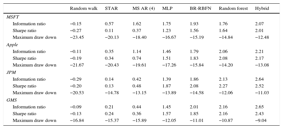
It is observed from Table 10 that the proposed MSAR (4) BR-RBFN model predictor performs significantly well than the other benchmark methods in terms of the information ratio. The proposed hybrid model surpasses the other non-linear models in terms of the maximum drawdown return value. The hybrid model and BR-RBFN have quite high risk-adjusted returns than other linear and nonlinear models – meaning that the estimated expected returns of the selected stocks are engaged with zero risks.
Buy/sell summaries of hybrid model trading performance.
| Random walk | STAR | MS AR (4) | MLP | BR-RBFN | Random forest | Hybrid | |
|---|---|---|---|---|---|---|---|
| MSFT | |||||||
| Information ratio | −0.15 | 0.57 | 1.62 | 1.75 | 1.93 | 1.76 | 2.07 |
| Sharpe ratio | −0.27 | 0.11 | 0.37 | 1.23 | 1.56 | 1.64 | 2.01 |
| Maximum draw down | −23.45 | −20.13 | −18.40 | −16.67 | −15.19 | −14.84 | −12.48 |
| Apple | |||||||
| Information ratio | −0.11 | 0.35 | 1.14 | 1.46 | 1.79 | 2.06 | 2.21 |
| Sharpe ratio | −0.19 | 0.34 | 0.74 | 1.51 | 1.83 | 2.08 | 2.17 |
| Maximum draw down | −21.67 | −20.43 | −19.61 | −17.26 | −15.84 | −14.20 | −13.08 |
| JPM | |||||||
| Information ratio | −0.29 | 0.14 | 0.42 | 1.39 | 1.86 | 2.13 | 2.64 |
| Sharpe ratio | −0.20 | 0.13 | 0.48 | 1.87 | 2.08 | 2.27 | 2.52 |
| Maximum draw down | −20.53 | −14.78 | −13.15 | −13.89 | −14.58 | −12.06 | −11.03 |
| GMS | |||||||
| Information ratio | −0.09 | 0.21 | 0.44 | 1.45 | 2.01 | 2.16 | 2.65 |
| Sharpe ratio | −0.13 | 0.24 | 0.36 | 1.57 | 1.85 | 2.16 | 2.43 |
| Maximum draw down | −16.84 | −15.37 | −15.89 | −12.05 | −11.01 | −10.87 | −9.04 |
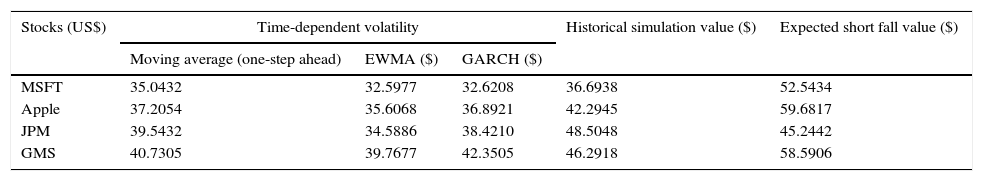
In this study, the daily stock prices open, high, low, close and technical indicators are utilized to provide a better forecasting tool for the individual investors. The hybrid model could provide the best signal based on the evaluated risk values for the individual investors who want to invest in the market. The hybrid model MSAR (4) BR-RBFN and buy/sell trading performance are represented in Tables 11 and 12, respectively. The parametric methods such as MA, EWMA, GARCH, historical simulation and expected shortfall are evaluated for the considered stock returns. The moving average (MA) model assumes that daily returns of the selected stocks get the same weights. The GMS provides higher risk value, approximately $40.73 higher than other three assets. When exponentially weighted moving average (EWMA) improves, there is better volatility forecast by applying more weights to the nearest recent trading days. Thus, the volatility forecast of GMS is $39.77. Generally, GARCH model not only allows the dynamic properties of volatilities but also promises to provide a better volatility forecast. The VaR of MSFT, Apple, GMS, and JPM are $32.62, $36.89, $38.42, and $42.35 respectively.
Forecasting risk value of hybrid model MSAR (4) BR-RBFN using the parametric method.
| Stocks (US$) | Time-dependent volatility | Historical simulation value ($) | Expected short fall value ($) | ||
|---|---|---|---|---|---|
| Moving average (one-step ahead) | EWMA ($) | GARCH ($) | |||
| MSFT | 35.0432 | 32.5977 | 32.6208 | 36.6938 | 52.5434 |
| Apple | 37.2054 | 35.6068 | 36.8921 | 42.2945 | 59.6817 |
| JPM | 39.5432 | 34.5886 | 38.4210 | 48.5048 | 45.2442 |
| GMS | 40.7305 | 39.7677 | 42.3505 | 46.2918 | 58.5906 |
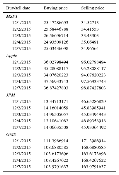
Forecasting buy/sell points using hybrid model MSAR (4) BR-RBFN.
| Buy/sell date | Buying price | Selling price |
|---|---|---|
| MSFT | ||
| 12/1/2015 | 25.47286693 | 34.52713 |
| 12/2/2015 | 25.58446788 | 34.41553 |
| 12/3/2015 | 26.56696714 | 33.43303 |
| 12/4/2015 | 24.93509126 | 35.06491 |
| 12/7/2015 | 25.03436098 | 34.96564 |
| Apple | ||
| 12/1/2015 | 36.02798494 | 96.02798494 |
| 12/2/2015 | 35.28088117 | 95.28088117 |
| 12/3/2015 | 34.07620223 | 94.07620223 |
| 12/4/2015 | 37.56933743 | 97.56933743 |
| 12/7/2015 | 36.87427803 | 96.87427803 |
| JPM | ||
| 12/1/2015 | 13.34713171 | 46.65286829 |
| 12/2/2015 | 14.16014059 | 45.83985941 |
| 12/3/2015 | 14.96505057 | 45.03494943 |
| 12/4/2015 | 13.10641082 | 46.89358918 |
| 12/7/2015 | 14.06635508 | 45.93364492 |
| GMS | ||
| 12/1/2015 | 111.3986914 | 171.3986914 |
| 12/2/2015 | 108.6880585 | 168.6880585 |
| 12/3/2015 | 103.6173696 | 163.6173696 |
| 12/4/2015 | 108.4267622 | 168.4267622 |
| 12/7/2015 | 103.9791637 | 163.9791637 |
Similarly, the historical simulation (HS) method relies on its past history; the expected next trading day return depends upon the expected past returns of the given stocks. This HS method effectively captures the non-linear dependencies in the stock returns. JPM and GMS stock returns have quite high VaR values as $48.50 and $46.29 respectively. The expected shortfall method is utilized to calculate the expected return for all the trading days of the selected stocks, which have more negative value than the VaR value of historical simulation. Basically, ES estimation needs a large number of samples to calculate the VaR value. The total number of samples for the selected stocks is 1257. Thus, the ES VaR value for MSFT, Apple, GMS and JPM are $52.54, $59.68 $58.59 and $45.24, respectively.
From Table 12, it is observed that the trading decision buy/sell points for the stocks MSFT, Apple, JPM and GMS have been forecasted using the hybrid model MSAR (4) BR-RBFN. For this analysis, the window size is decided at 5, based on the analysis that the potential stocks could easily be identified for the investment.
5ConclusionsThe findings showed that the proposed hybrid model MSAR (4) BR-RBFN is significantly improving the one-step-ahead predictive performance for the stock returns MSFT, Apple, GMS, and JPM. Additionally, this hybrid approach overcomes the limitations of single model predictability of the considered stock returns. Also, with the minimum error measures, this hybrid model MSAR (4)-BRRBFN can predict the future stock investment decisions based on the buy/sell trading signal for the given stock returns in the trading market. It is noteworthy to mention that the proposed MSAR (4)-BRRBFN predictor inherits its network generalization and overcomes the plague of network overfitting and overtraining.
Moreover, the experimental results of value at risk explores that the evaluation of investment risk and the investment trading strategy, providing a better investment risk accuracy with the lowest risk errors using the parametric methods such as MA, EWMA, GARCH and historical simulation in favour of the considered stock returns. The comparative results embody that the predictive efficacy of the proposed hybrid model significantly surpassed its pure linear and non-linear models. Thus, this model proves its effective predictive power and its reliability in terms of capturing the non-linear patterns with minimum error values. Thus, this predictive tool provides an information signal to the individual investors who are willing to forge in the market. So, this novel architecture highlights the importance of hybrid modelling and also provides a good financing tool for the individual investors.
Funding resourceThis research was supported by the Indian Council of Social Science Research (ICSSR), made possible in part by the Ministry of Human Resource Development (MHRD) and centrally administrated Doctoral Fellowship program under the grant No: RFD/2014-2015/GEN/ECO/061.
The author is grateful to the Editor and the reviewers for their valuable comments that facilitated the quality enhancement of this study.

