


After the implementation of MiFID (I and II), competition is a reality in all the European Cash Markets. A natural consequence of competition is that order flow is fragmented in different type of venues. This paper focuses on the consequences of fragmentation on the local market liquidity of the Spanish Stock Exchange (hereafter SSE). Our main result shows that, for our sample, fragmentation is relevant determining the cost of liquidity. Following the analysis of Degryse et al. (2014), the linear component of fragmentation has a positive and significant effect on liquidity (reduces spreads and increases Kyle's Lambda) and the quadratic term has a negative and significant effect on liquidity (increases spreads and reduces Kyle's Lambda). So, fragmentation is good for liquidity but beyond a given level of fragmentation, increasing it is worse for the liquidity of the regulated market.
Financial Market Fragmentation is one of the important issues during the last decade. Financial markets have evolved from a natural monopolistic position in Europe to a competitive environment where fragmentation is a key ingredient. Competition is one of the main tasks of Markets in Financial Instruments Directive (MiFID). MiFID defines three different alternative trading venues. First, the Regulated Markets are the traditional cash markets where transactions are done through matching buy and sell orders in a Limit Order Book with a diversity of traders. Second, the Multi Trading Facilities (MTF) that provide liquidity in the same way than regulated markets but with lower transparency requirements.2 MTF can offer lit or dark liquidity.3 Last, the Sistematic Internalizers (SI) that are investment firms who could match “buy” and “sell” orders from clients in-house. Instead of sending orders to a RM or a MTF, SIs can match orders on its own book.
The expected positive effects of increasing the level of competition should be the reduction of trading fees and an increase of liquidity through the reduction of execution cost. The negative one could be the fragmentation of supply and demand and its consecuences in volatility and execution cost. As result of fragmentation, it is not clear the final effect of competition on different liquidity measures. Competition is possible if competitors can improve the execution conditions. These execution conditions includes an improvement of the liquidity conditions, the quality of the trading technology (e.g. the speed of execution), the number of securities traded or make and take fees and clearing and settlement costs among others.
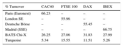
Looking at European Markets and as a consequence of MiFID, fragmentation is a reality. Additionally, Table 1 summarizes the distribution of the turnover in Europe from July 6th to 10th of 2015. The Total column shows the percentage distribution only among Lit markets. BATS Chi-X transacts 24.25% of the lit markets total volume. If we look at the other columns we see the same concept but only considering stocks included in each index. Table 1 main conclusion is that BATS Chi-X is capturing around 30% of the total lit turnover. The rest till 100% is dark.
Market fragmentation in lit markets. This table shows the distribution of turnover of the constituents of four selected European Indices from July 6th to 10th of 2015. We only include market turnover in lit markets.
| % Turnover | CAC40 | FTSE 100 | DAX | IBEX |
|---|---|---|---|---|
| Paris (Euronext) | 66.23 | – | – | – |
| London SE | – | 55.96 | – | – |
| Deutsche Börse | – | – | 55.45 | – |
| Madrid (SSE) | – | – | – | 66.75 |
| BATS Chi-X | 26.25 | 27.06 | 31.83 | 27.99 |
| Turquoise | 5.34 | 15.55 | 11.51 | 5.26 |
Source: Fidessa.
Focusing on empirical papers, on one side Bennett and Wei (2006) show that the assets that move from less consolidated market like NASDAQ to a more consolidated ones like NYSE reduce the execution cost. On the other, the greatest part of the papers found positive results on the effect of fragmentation on liquidity but we should highlight that this effect does not hold for the whole sample. Among others, Chlistalla and Lutat (2011) observe an increases in liquidity of the most actively traded stocks in the sample when these asset are trading in Chi-X and in Euronext-Paris. But this positive result does not hold for the less traded stocks. Another example is Fioravanti and Gentile (2011). With the assets of Stoxx Europe 50 Index, they find that the trading in the RM and the MTFs increases liquidity (narrowing quoted spreads and increasing quoted depth at the best prices) but the increase in fragmentation reduces informational efficiency. Gresse (2012) examines fragmentation of European markets analyzing the stocks included in the FTSE-100, CAC-40, and SBF-120 (the non-CAC-40 components of the index) before and after the implementation of the MiFID. The author finds that visible fragmentation narrows spreads and increases depth or does not affect it.
Last, the research closely related to ours is Degryse et al. (2014). They use a sample of Dutch stocks during 4 years (January 2006 to the end of 2009). Therefore, the sample includes a period with fragmentation and a period without it. Degryse et al. (2014) construct daily averages with information that covers the whole limit order book of the stocks during the sample period using intraday data. They measure liquidity with three alternative measures. First, they calculate quoted spreads and quoted depth at the best prices. Secondly, they use “Depth(X)”. This liquidity measure aggregates the effective volume posted at 10, 20, 30, 40, and 50 basis points around the mid point. Also, they distinguish between visible and dark trading calculating fragmentation level in both scenarios. The authors use one minus Herfindahl–Hirschman Index (1-HHI) to measure fragmentation.
They observe that the effect of fragmentation on liquidity shows an inverted U-shape. Their results imply that fragmentation improves liquidity but beyond a specific level of fragmentation it becomes worse. Moreover, the authors find that visible fragmentation decrease “local liquidity” (liquidity at traditional stock exchanges). Therefore, investors that can only access to national market are worse off in a fragmented market environment.
Our results follows the previous ones, we find that fragmentation plays a similar role in SSE as the ones it plays in other stock exchanges. Fragmentation is relevant determining the cost of liquidity. Linear component of fragmentation has a positive and significant effect on liquidity (reduces spreads and increases Kyle's Lambda) and the quadratic term has negative and significant effect on liquidity (increases spreads and reduces Kyle's Lambda). So, fragmentation is good for liquidity till some point. Beyond this level of fragmentation, increasing the fragmentation level is worse for the liquidity of the regulated market. For SSE, the maximum improvement of QSp is when the level of fragmentation is 21.5%. This represents a decrease of 2.42 basis points. Regarding DWQSp the fragmentation level of the maximum decrease is at 19% with 5.86 basis points. Last, the highest improvement of lambda is at 25.5% with a 11.20% higher level of lambda. These results are robust to controlling for market-wide liquidity effects (Chordia et al., 2000).
2The market and the datasetOur dataset contains 21 Spanish stocks listed on SSE. These stocks are the most important constituents of the Spanish Index, the IBEX-35© and belong to the Index during our sample period. These stocks can be traded in alternative venues. The SSE handles the most important part of trading activity. Trading is continuous from 9:00 am to 5:30 pm GMT+1, with call auctions at the opening (8:30–9:00am) and closing (5:30–5:35pm).
Our database covers 5 years (from January 2010 to February 2015) of volume daily data of alternative trading venues. The first group is the RMs. We include SSE, Euronext, Xetra International Market and NASDAQ OMX. Those markets are organized through Limit Order Books where the whole market participants post limit orders providing liquidity. Although, we can observe a diversity of RMs, the associated effective volume of Euronext, Xetra International Market and NASDAQ OMX is negligible for our data set.4 The second group are the lit Multi Trading Facilities (MTF) that provide liquidity in the same way (e.g. through LOBs). Chi-X, Bats Europe, and Turquoise are the members of this group. This group is the main responsible of the fragmentation in our sample. The third group contains MTFs with completely hidden liquidity (e.g. dark pools), Systematic Internalizers and the Over The Counter market.5 Unfortunately, our dataset does not include volume of such competitors.
The SSE handles the most important part of trading activity.6 Trading is continuous from 9:00am to 5:30pm GMT+1, with call auctions at the opening (8:30–9:00am) and closing (5:30–5:35pm). Our database covers 5 years (from January 2010 to February 2015) of daily data that includes:
2.1Liquidity variables- 1.
Quoted Spread (QSp) is the average of the intraday quoted spreads. Intraday quoted spreads are calculated in the standard way each time there is a change in one of the five best Ask or Bid prices. Qsp is measured in basis points.
- 2.
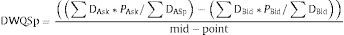
Depth Weighted Quoted Spread (DWQSp) is the average of the intraday depth weighted quoted spreads. Intraday depth weighted quoted spreads is calculated as:
The SSE calculates DWQSp each time there is a change in one of the five best Ask or Bid prices. DWQSp is measured in basis points. - 3.
Lambda(λ) is the result of calculating the amount of money needed to move the mid-price 100 basis points on both sides of the LOB. The market calculates the effective volume needed to sweep all the volume of the five best positions at the Bid (Ask). At the same time, the market calculates the movement of the prices in basis points. Next, the market does an average of the effective and the percentages for the Ask and the Bid side. Last, the market normalizes this figure to 100 basis points. The result is an ex-ante liquidity measure that is comparable for different stocks and that collect all the available information. The market measures Lambda each time there is a change in one of the five best Ask or Bid prices. Næs and Skjeltorp (2006) or Martínez et al. (2004) among others, using information of the consolidated limit order book build same style measure that shows the properties of liquidity measured beyond the quoted spreads.
Fragmentation (Frag) is proxy for market fragmentation. We calculate
where EffSSE is the effective volume transacted in SSE and TotalEff includes the effective volume traded in any of these venues: SSE, Turquoise, Chi-X Europe, Nasdaq OMX Europe, NYSE Arca Europe, BATS Europe, Equiduct and Xetra International Market. We also calculate HHI as Degryse et al. (2014) but we use Frag in the analysis given that we only consider liquidity measures of SSE. However, given that fragmentation of SSE is below 50% Frag and 1-HHI are highly correlated and the results using 1-HHI are equal to the ones using Frag in sign and significance.2.3Control variables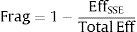
We use the classic control variables used in the literature:
- 1.
Volatility: we calculate volatility as the absolute value of the daily return for each firm; we do not consider intraday estimations because of the lack of intraday data.
- 2.
Size: we use the logarithm of daily market value for each firm.
- 3.
Effective volume: we use the logarithm of total effective volume in Euros traded in all the venues for each firm.
- 4.
The inverse of the closing price for each firm.
Fig. 1 shows the behavior of the fragmentation variable in our sample. First, the path shows how fragmentation has been increasing during the sample from 1.25% to 24%. The evolution of fragmentation is common to other papers and samples like Degryse et al. (2014) or Fioravanti and Gentile (2011). Moreover, we can clearly observe 3 different periods: (i) before Jan 2012, (ii) 2012 and (iii) after December 2012. We will use these different subsamples to re-estimate our model and obtain additional insights about fragmentation and liquidity measures.

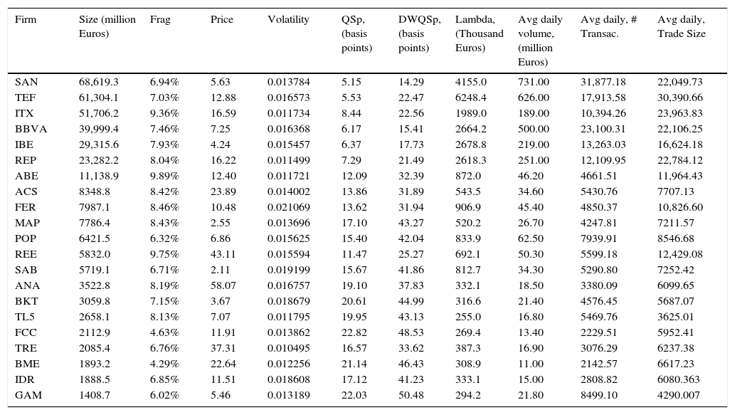
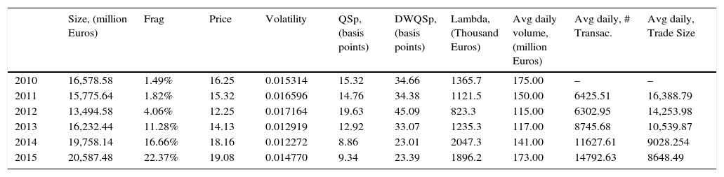
Tables 2 and 3 show some stylized facts of our sample. Table 2 shows the diversity in size of the stocks included in the sample (largest company, Santander Bank is almost 50 times the smallest Gamesa). These differences in size can also be observed in the three measures of liquidity (larger size is associated with higher liquidity) and in the activity measures: average daily volume measured in million of euros, average daily number of transactions and average daily trade size (larger size is associated with higher activity measures). We do not observe important differences in fragmentation. The average level of fragmentation is around 7.5% for the whole sample (firm and years) and there are no significant differences if we look at size. Table 3 shows the evolution of the main variables over the years. We can see a continuous increase in fragmentation and at the same time an increase in liquidity (with the exception of 2012).7 We can also observe a steady decrease in trade size.
Firms included in the sample. This table includes the main stylized facts of the firms included in the sample. We rank the stocks by average market cap.
| Firm | Size (million Euros) | Frag | Price | Volatility | QSp, (basis points) | DWQSp, (basis points) | Lambda, (Thousand Euros) | Avg daily volume, (million Euros) | Avg daily, # Transac. | Avg daily, Trade Size |
|---|---|---|---|---|---|---|---|---|---|---|
| SAN | 68,619.3 | 6.94% | 5.63 | 0.013784 | 5.15 | 14.29 | 4155.0 | 731.00 | 31,877.18 | 22,049.73 |
| TEF | 61,304.1 | 7.03% | 12.88 | 0.016573 | 5.53 | 22.47 | 6248.4 | 626.00 | 17,913.58 | 30,390.66 |
| ITX | 51,706.2 | 9.36% | 16.59 | 0.011734 | 8.44 | 22.56 | 1989.0 | 189.00 | 10,394.26 | 23,963.83 |
| BBVA | 39,999.4 | 7.46% | 7.25 | 0.016368 | 6.17 | 15.41 | 2664.2 | 500.00 | 23,100.31 | 22,106.25 |
| IBE | 29,315.6 | 7.93% | 4.24 | 0.015457 | 6.37 | 17.73 | 2678.8 | 219.00 | 13,263.03 | 16,624.18 |
| REP | 23,282.2 | 8.04% | 16.22 | 0.011499 | 7.29 | 21.49 | 2618.3 | 251.00 | 12,109.95 | 22,784.12 |
| ABE | 11,138.9 | 9.89% | 12.40 | 0.011721 | 12.09 | 32.39 | 872.0 | 46.20 | 4661.51 | 11,964.43 |
| ACS | 8348.8 | 8.42% | 23.89 | 0.014002 | 13.86 | 31.89 | 543.5 | 34.60 | 5430.76 | 7707.13 |
| FER | 7987.1 | 8.46% | 10.48 | 0.021069 | 13.62 | 31.94 | 906.9 | 45.40 | 4850.37 | 10,826.60 |
| MAP | 7786.4 | 8.43% | 2.55 | 0.013696 | 17.10 | 43.27 | 520.2 | 26.70 | 4247.81 | 7211.57 |
| POP | 6421.5 | 6.32% | 6.86 | 0.015625 | 15.40 | 42.04 | 833.9 | 62.50 | 7939.91 | 8546.68 |
| REE | 5832.0 | 9.75% | 43.11 | 0.015594 | 11.47 | 25.27 | 692.1 | 50.30 | 5599.18 | 12,429.08 |
| SAB | 5719.1 | 6.71% | 2.11 | 0.019199 | 15.67 | 41.86 | 812.7 | 34.30 | 5290.80 | 7252.42 |
| ANA | 3522.8 | 8.19% | 58.07 | 0.016757 | 19.10 | 37.83 | 332.1 | 18.50 | 3380.09 | 6099.65 |
| BKT | 3059.8 | 7.15% | 3.67 | 0.018679 | 20.61 | 44.99 | 316.6 | 21.40 | 4576.45 | 5687.07 |
| TL5 | 2658.1 | 8.13% | 7.07 | 0.011795 | 19.95 | 43.13 | 255.0 | 16.80 | 5469.76 | 3625.01 |
| FCC | 2112.9 | 4.63% | 11.91 | 0.013862 | 22.82 | 48.53 | 269.4 | 13.40 | 2229.51 | 5952.41 |
| TRE | 2085.4 | 6.76% | 37.31 | 0.010495 | 16.57 | 33.62 | 387.3 | 16.90 | 3076.29 | 6237.38 |
| BME | 1893.2 | 4.29% | 22.64 | 0.012256 | 21.14 | 46.43 | 308.9 | 11.00 | 2142.57 | 6617.23 |
| IDR | 1888.5 | 6.85% | 11.51 | 0.018608 | 17.12 | 41.23 | 333.1 | 15.00 | 2808.82 | 6080.363 |
| GAM | 1408.7 | 6.02% | 5.46 | 0.013189 | 22.03 | 50.48 | 294.2 | 21.80 | 8499.10 | 4290.007 |
Averages by year. This table shows the average of the relevant variables by year.
| Size, (million Euros) | Frag | Price | Volatility | QSp, (basis points) | DWQSp, (basis points) | Lambda, (Thousand Euros) | Avg daily volume, (million Euros) | Avg daily, # Transac. | Avg daily, Trade Size | |
|---|---|---|---|---|---|---|---|---|---|---|
| 2010 | 16,578.58 | 1.49% | 16.25 | 0.015314 | 15.32 | 34.66 | 1365.7 | 175.00 | – | – |
| 2011 | 15,775.64 | 1.82% | 15.32 | 0.016596 | 14.76 | 34.38 | 1121.5 | 150.00 | 6425.51 | 16,388.79 |
| 2012 | 13,494.58 | 4.06% | 12.25 | 0.017164 | 19.63 | 45.09 | 823.3 | 115.00 | 6302.95 | 14,253.98 |
| 2013 | 16,232.44 | 11.28% | 14.13 | 0.012919 | 12.92 | 33.07 | 1235.3 | 117.00 | 8745.68 | 10,539.87 |
| 2014 | 19,758.14 | 16.66% | 18.16 | 0.012272 | 8.86 | 23.01 | 2047.3 | 141.00 | 11627.61 | 9028.254 |
| 2015 | 20,587.48 | 22.37% | 19.08 | 0.014770 | 9.34 | 23.39 | 1896.2 | 173.00 | 14792.63 | 8648.49 |
In our basic model, we regress liquidity dependent variables on our measure of fragmentation and fragmentation squared. We use a classic set of control variables for each firm: volatility (the absolute value of the daily return), size (the logarithm of daily market capitalization), effective volume (the logarithm of total effective volume in Euros traded in all the venues) and the inverse of the closing price.

As dependent variables, we use QSp and DWQSp measured in basis points and the logarithm of Kyle's Lambda. The three endogenous variables are daily averages as provided by the SSE.
As exogenous variables we use Frag and the square of fragmentation (Frag2) to observe if the fragmentation effect is not linear. Unfortunately, we do not have data about messages traffic as Degryse et al. (2014). However, Chakrabarty et al. (2015) show that HFT activity did not change substantially between 2011 and 2013 in the SSE. So we can assume that the possible effect of HFT activity is not relevant for our results. The regressions use 1315 trading days for 21 stocks from January 2010 to February 2015.
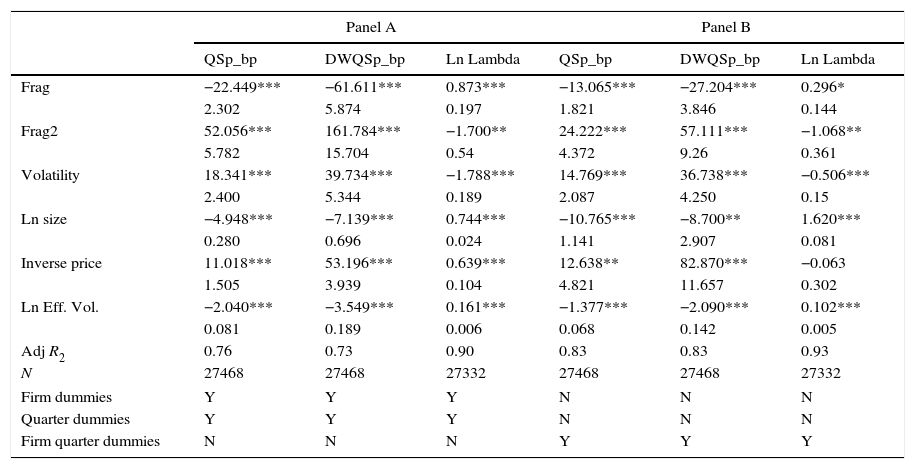
We estimate the basic equation using time series regression with quarter and firm dummies correcting using Newey–West (HAC) corrected standard errors with five lags. Table 4 includes the results of our basic equation. Panel A includes the results of the basic equation with dummies for firm and quarter while Panel B regressions include quarter*firm dummies. Quarter*firm dummies are used to control for the changes in market structure and the possible interaction effects of this changes with the different companies.
This table shows the results of the next regression. Liqit=α+βFrag*Fragit+βFrag2*Frag2it+γ*ControlV1.
| Panel A | Panel B | |||||
|---|---|---|---|---|---|---|
| QSp_bp | DWQSp_bp | Ln Lambda | QSp_bp | DWQSp_bp | Ln Lambda | |
| Frag | −22.449*** | −61.611*** | 0.873*** | −13.065*** | −27.204*** | 0.296* |
| 2.302 | 5.874 | 0.197 | 1.821 | 3.846 | 0.144 | |
| Frag2 | 52.056*** | 161.784*** | −1.700** | 24.222*** | 57.111*** | −1.068** |
| 5.782 | 15.704 | 0.54 | 4.372 | 9.26 | 0.361 | |
| Volatility | 18.341*** | 39.734*** | −1.788*** | 14.769*** | 36.738*** | −0.506*** |
| 2.400 | 5.344 | 0.189 | 2.087 | 4.250 | 0.15 | |
| Ln size | −4.948*** | −7.139*** | 0.744*** | −10.765*** | −8.700** | 1.620*** |
| 0.280 | 0.696 | 0.024 | 1.141 | 2.907 | 0.081 | |
| Inverse price | 11.018*** | 53.196*** | 0.639*** | 12.638** | 82.870*** | −0.063 |
| 1.505 | 3.939 | 0.104 | 4.821 | 11.657 | 0.302 | |
| Ln Eff. Vol. | −2.040*** | −3.549*** | 0.161*** | −1.377*** | −2.090*** | 0.102*** |
| 0.081 | 0.189 | 0.006 | 0.068 | 0.142 | 0.005 | |
| Adj R2 | 0.76 | 0.73 | 0.90 | 0.83 | 0.83 | 0.93 |
| N | 27468 | 27468 | 27332 | 27468 | 27468 | 27332 |
| Firm dummies | Y | Y | Y | N | N | N |
| Quarter dummies | Y | Y | Y | N | N | N |
| Firm quarter dummies | N | N | N | Y | Y | Y |
The dependent variables are QSp and DWQSp, measured in basis points, and the logarithm of Kyle's Lambda measured as the amount of money needed to move the mid price of an asset 100 basis points. The three endogenous variables are daily averages calculated by the SSE. Frag is the degree of market fragmentation (1-eff_SSE/tot_eff) and Frag2 is Frag squared. The control variables are volatility (absolute value of the daily return), size (logarithm of daily market capitalization), Effective Volume (logarithm of total effective volume traded) and the inverse of the closing price. We estimate the basic equation using time series regression with quarter and firm dummies correcting using Newey–West (HAC) corrected standard errors with five lags. Panel A includes the results of the basic equation with dummies for firm and quarter while Panel B regressions include quarter*firm dummies. The regressions use 1315 trading days for 21 stocks from January 2010 to February 2015. Below each coefficient, we show the standard errors and the R2 of the regression. ***, **, and * denote significance at the 0.1, 1, and 5% levels, respectively.
Looking at results of Table 4 panel A, we can conclude that fragmentation is a relevant determinant of the cost of liquidity. The linear component of fragmentation has a positive and significant effect on liquidity (reduces spreads and increases Kyle's Lambda) and the quadratic term has a negative and significant effect on liquidity (increases spreads and reduces Kyle's Lambda). On one side, the signs are in the same direction than Degryse et al. (2014) although the positive effect of Frag2 is larger. On the other our results on QSp are closer to O’Hara and Ye (2011) whose find a benefit from fragmentation close to 3 basis points.
Our main result is that the linear component of fragmentation improves liquidity (QSp. DWQSp and Kyle's Lambda) while the quadratic term worsens liquidity. The conclusion of Table 4 is that fragmentation is good for liquidity up to a point. Beyond it, increasing the level of fragmentation worse liquidity in the regulated market. In particular, the maximum improvement of QSp is attained at a level of fragmentation of 21.5%. At this level of fragmentation, QSp is 2.42 basis points lower than with zero fragmentation.
Regarding DWQSp the fragmentation level of the maximum decrease is at 19% and it is associated with a lower of DWQSp by 5.86 basis points. Lastly, the highest improvement of lambda is at 25.5% with a 11.20% higher level of lambda. We can also observe that the coefficients of fragmentation are higher when we use DWQSp that when we use QSp as endogenous variable. The only reason is that DWQSp values are larger than the QSP ones. The sign and significance of the control variables are as expected from other papers in the literature.
Next, we represent graphically the results of Table 4. Fig. 2 shows the impact of fragmentation on liquidity. Given the coefficients of the basic equation, we calculate the impact of a level of fragmentation on our liquidity measures. We compute:
 The impact of fragmentation on QSp and DWQSp of different levels of fragmentation using the point estimates of Table 4 panel A. QSp=βFrag*Frag+βFrag2*Frag2. (B) The impact of different levels of fragmentation on Ln Lambda with the results of Table 4 panel A. Ln Lambda=βFrag*Frag+βFrag2*Frag2, Lambda%=expLn Lambda−1.")
 The impact of fragmentation on QSp and DWQSp of different levels of fragmentation using the point estimates of Table 4 panel A. QSp=βFrag*Frag+βFrag2*Frag2. (B) The impact of different levels of fragmentation on Ln Lambda with the results of Table 4 panel A. Ln Lambda=βFrag*Frag+βFrag2*Frag2, Lambda%=expLn Lambda−1.")
Impact of an increase in fragmentation on liquidity measures. (A) The impact of fragmentation on QSp and DWQSp of different levels of fragmentation using the point estimates of Table 4 panel A. QSp=βFrag*Frag+βFrag2*Frag2. (B) The impact of different levels of fragmentation on Ln Lambda with the results of Table 4 panel A. Ln Lambda=βFrag*Frag+βFrag2*Frag2, Lambda%=expLn Lambda−1.
L=βFrag*Frag+βFrag2*Frag2
Looking at the figures and observing the final level of fragmentation in the sample, we can conclude that higher level of fragmentation is going to increase the immediacy cost and Lambda and as a consequence liquidity will be reduced. This point is particularly important if we consider the level of fragmentation at the end of our sample that, as is shown in Table 3, was 22.37%.
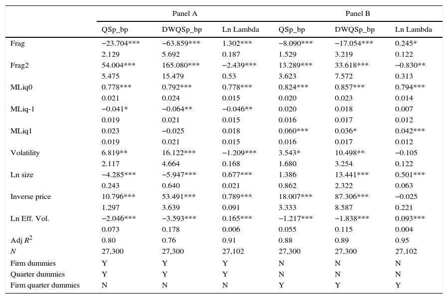
3.2Controlling for commonality in liquidity across stocksPrevious research has demonstrated the existence of market-wide factors in liquidity determination (Chordia et al., 2000 for example). Thus it is possible that our regressions suffer from omitted variable problems given that they do not contain these market-level effects. To check this we modified our regression specification in the following way:
where MLiq is the average value of liquidity across all stocks in the sample at a particular day. Thus the new specification allows market-wide liquidity to affect stock level liquidity. To allow for dynamics in this relationship we also include the first lead and the first lag of the market liquidity variable. Table 5 contains the results from these estimations. As expected, contemporaneous aggregated liquidity measures are positive and significant. Regarding the fragmentation coefficients, the results are similar in terms of sign and value to the ones we obtained with Eq. (1). This result confirms the accuracy of the previous results.
The dependent variables are QSp and DWQSp, measured in basis points, and the logarithm of Kyle's Lambda measured as the amount of money needed to move the mid price of an asset 100 basis points. The three endogenous variables are daily averages calculated by the SSE. Frag is the degree of market fragmentation (1-eff_SSE/tot_eff) and Frag2 is Frag squared. MLiq is the average value of liquidity across all stocks in the sample at a particular day. The control variables are volatility (absolute value of the daily return), size (logarithm of daily market capitalization), Effective Volume (logarithm of total effective volume traded) and the inverse of the closing price. We estimate the basic equation using time series regression with quarter and firm dummies correcting using Newey–West (HAC) corrected standard errors with five lags. Panel A includes the results of the basic equation with dummies for firm and quarter while Panel B regressions include quarter*firm dummies. The regressions use 1315 trading days for 21 stocks from January 2010 to February 2015. Below each coefficient, we show the standard errors and the R2 of the regression. ***, **, and * denote significance at the 0.1, 1, and 5% levels, respectively.
| Panel A | Panel B | |||||
|---|---|---|---|---|---|---|
| QSp_bp | DWQSp_bp | Ln Lambda | QSp_bp | DWQSp_bp | Ln Lambda | |
| Frag | −23.704*** | −63.859*** | 1.302*** | −8.090*** | −17.054*** | 0.245* |
| 2.129 | 5.692 | 0.187 | 1.529 | 3.219 | 0.122 | |
| Frag2 | 54.004*** | 165.080*** | −2.439*** | 13.289*** | 33.618*** | −0.830** |
| 5.475 | 15.479 | 0.53 | 3.623 | 7.572 | 0.313 | |
| MLiq0 | 0.778*** | 0.792*** | 0.778*** | 0.824*** | 0.857*** | 0.794*** |
| 0.021 | 0.024 | 0.015 | 0.020 | 0.023 | 0.014 | |
| MLiq-1 | −0.041* | −0.064** | −0.046** | 0.020 | 0.018 | 0.007 |
| 0.019 | 0.021 | 0.015 | 0.016 | 0.017 | 0.012 | |
| MLiq1 | 0.023 | −0.025 | 0.018 | 0.060*** | 0.036* | 0.042*** |
| 0.019 | 0.021 | 0.015 | 0.016 | 0.017 | 0.012 | |
| Volatility | 6.819** | 16.122*** | −1.209*** | 3.543* | 10.498** | −0.105 |
| 2.117 | 4.664 | 0.168 | 1.680 | 3.254 | 0.122 | |
| Ln size | −4.285*** | −5.947*** | 0.677*** | 1.386 | 13.441*** | 0.501*** |
| 0.243 | 0.640 | 0.021 | 0.862 | 2.322 | 0.063 | |
| Inverse price | 10.796*** | 53.491*** | 0.789*** | 18.007*** | 87.306*** | −0.025 |
| 1.297 | 3.639 | 0.091 | 3.333 | 8.587 | 0.221 | |
| Ln Eff. Vol. | −2.046*** | −3.593*** | 0.165*** | −1.217*** | −1.838*** | 0.093*** |
| 0.073 | 0.178 | 0.006 | 0.055 | 0.115 | 0.004 | |
| Adj R2 | 0.80 | 0.76 | 0.91 | 0.88 | 0.89 | 0.95 |
| N | 27,300 | 27,300 | 27,102 | 27,300 | 27,300 | 27,102 |
| Firm dummies | Y | Y | Y | N | N | N |
| Quarter dummies | Y | Y | Y | N | N | N |
| Firm quarter dummies | N | N | N | Y | Y | Y |
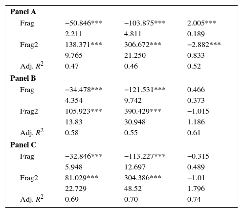
Endogeneity is clearly a concern in attempting to understand how fragmentation drives market liquidity. It is possible that market liquidity affects fragmentation at the same time that fragmentation is driving market liquidity. In this subsection, we report results from the use of instrumental variables to control for possible endogeneity. We use the lagged values of the two fragmentation variables to re-estimate our model. The regressions are estimated following a standard Instrumental Variables approach using lagged values of frag and frag2 as instruments. Results are in Table 6. Concentrating on the results involving all stocks, it is clear that, if anything, the IV results are stronger than the results of Table 4. All IV coefficients are of the same sign, but larger in magnitude than their OLS counterparts. The IV standard errors are larger, but the vast majority of the estimates retain statistical significance at the 1% level for the benchmark IV model.
Robust IV.
| Panel A | |||
| Frag | −50.846*** | −103.875*** | 2.005*** |
| 2.211 | 4.811 | 0.189 | |
| Frag2 | 138.371*** | 306.672*** | −2.882*** |
| 9.765 | 21.250 | 0.833 | |
| Adj. R2 | 0.47 | 0.46 | 0.52 |
| Panel B | |||
| Frag | −34.478*** | −121.531*** | 0.466 |
| 4.354 | 9.742 | 0.373 | |
| Frag2 | 105.923*** | 390.429*** | −1.015 |
| 13.83 | 30.948 | 1.186 | |
| Adj. R2 | 0.58 | 0.55 | 0.61 |
| Panel C | |||
| Frag | −32.846*** | −113.227*** | −0.315 |
| 5.948 | 12.697 | 0.489 | |
| Frag2 | 81.029*** | 304.386*** | −1.01 |
| 22.729 | 48.52 | 1.796 | |
| Adj. R2 | 0.69 | 0.70 | 0.74 |
The dependent variables are QSp and DWQSp, measured in basis points, and the logarithm of Kyle's Lambda measured as the amount of money needed to move the mid price of an asset 100 basis points. The three endogenous variables are daily averages calculated by the SSE. Frag is the degree of market fragmentation (1-eff_SSE/tot_eff) and Frag2 is Frag squared. The control variables are volatility (absolute value of the daily return), size (logarithm of daily market capitalization), Effective Volume (logarithm of total effective volume traded) and the inverse of the closing price. The regressions are Instrumental Variables approach using lagged values of frag and frag2 Panel A includes asset fixed effects, Panel B includes asset fixed effects and quarter dummies and Panel C includes asset fixed effects and firm*quarter dummies. The regressions use 1315 trading days for 21 stocks from January 2010 to February 2015. Below each coefficient, we show the standard errors and the R2 of the regression. ***, **, and * denote significance at the 0.1, 1, and 5% levels, respectively.
In this paper we show that fragmentation plays a similar role in SSE as the ones it plays in other stock exchanges. Fragmentation is a relevant determinant of the cost of liquidity. The linear component of fragmentation has a positive and significant effect on liquidity (reduces spreads and increases Kyle's Lambda) and the quadratic term has negative and significant effect on liquidity (increases spreads and reduces Kyle's Lambda). So, fragmentation is good for liquidity up to a point. Beyond this level, increasing fragmentation worsens liquidity in the regulated market. For SSE, the maximum improvement of QSp is when the level of fragmentation is 21.5%. This represents a decrease of 2.42 basis points. Regarding DWQSp the fragmentation level of the maximum decrease is at 19% with 5.86 basis points. Last, the highest improvement of lambda is at 25.5% with a 11.20% higher level of lambda.
I am grateful for comments and useful discussions from B. Alonso, I. Filippou, J. Hernani, J. Penalva and J. Yzaguirre and the seminar participants at Universidad Carlos III. Mikel Tapia acknowledges financial support from Ministerio de Ciencia y Tecnologia grant ECO2012-35023. The paper has benefited from the comments of the participants at 24th Finance Forum (CUNEF, Madrid) and the seminar participants at Universidad Carlos III. The opinions expressed in this paper are those of the author exclusively.
MiFID II equalizes the ex-ante and post-trading transparency level of RM and MTF.
MTF that offer dark liquidity are named Dark Pools.
At the end of 2014, there is no volume associated with other RMs although traders can transact.
Davies (2008) provides a good description of these trading venues.

