


This paper presents the analysis of the monthly portfolio holdings and daily returns of a large sample of Spanish domestic equity funds to test the potential manipulation of portfolios in mandatory reports. The comparison between the return of the fund portfolio holdings and the observed fund return reveals that only a low percentage of filings may be classified as window-dressed portfolios. These portfolios are dispersed across funds and fund managers, but they are clustered over three specific quarters that coincide with bear market months. The results seem to indicate that although window dressing is not a widespread practice in the Spanish market, there is evidence to suggest that mutual funds employ this trading strategy as a response to poor past performance.
There is an evident worldwide development and growth of the mutual fund industry. The importance of this industry is not only economic but also social, given the magnitude of the assets under management and household participation. Therefore, there is an increasing need to ensure that investors receive reliable information to make decisions and that they are adequately protected against abusive mutual fund practices.
As a result of this potential manipulation, the disclosed portfolios may reveal an uninformative image of the recent management of the fund, thus rising agency problems between fund managers and investors. Managers are motivated to improve the disclosed portfolio image to create the impression that the fund is performing relatively well to attract larger money inflows from investors who mostly make investment decisions according to recent performance records (Chevalier and Ellison, 1997; Sirri and Tufano, 1998, among others).
According to current legislation of collective investment in Spain, mutual fund managers must reveal their portfolio holdings to shareholders each quarter.1 Despite these disclosure requirements to ensure that investors are informed, fund managers might have incentives to use trading strategies to alter the reliability of their reports. In this case, the disclosed information is not useful for investor decisions because the information is simply a snapshot of the securities portfolio at a particular date; it does not necessarily provide information about the securities held throughout the quarter. Unfortunately, this practice of portfolio manipulation is difficult for mutual fund authorities to detect, and even more difficult for individual investors, given the high quality information needed to carry out comprehensive analyses on this matter.
The objective of this paper is to examine mutual fund returns and portfolio holdings in a sample of Spanish equity funds to test the existence of intentional portfolio manipulation around portfolio disclosures. This phenomenon is broadly known as window dressing hypothesis. Some of the studies in this field are: Lakonishok et al. (1991), Musto (1999), He et al. (2004), Ng and Wang (2004), Meier and Schaumburg (2006), and Morey and O’Neal (2006).
To our knowledge, this study is the first that examines fund returns and portfolio holdings to analyze the window-dressing hypothesis in a European fund industry. Then, we expect to obtain answers to the following questions: Do Spanish equity funds window dress their portfolios? In this case, is the use of window-dressing strategies by Spanish equity funds persistent? And, have window-dressed portfolios some common characteristics?
The results suggest that the window-dressing practice is not very common in Spanish equity funds during the period analyzed. This perception is confirmed in the study of common characteristics of window-dressed portfolios because the results do not reveal signs of clustering around funds and fund management companies. However, the findings also show that mutual funds might use window-dressing practices to mitigate past losses. Finally, the results confirm that window-dressed portfolios are clustered over bear market periods.
The rest of the paper is organized as follows: Section 2 reviews the literature, Section 3 describes the databases used in the analysis. Section 4 explains the methodology. Section 5 shows the main empirical results, and Section 6 presents the main conclusions of the research.
2Literature review and research questionsIn an attempt to find evidence of window dressing in mutual funds, several studies have employed the traditional approach of analyzing the trading activity of mutual funds through the comparison of portfolio holdings (Lakonishok et al., 1991; Basarrate and Rubio, 1994; Eakins and Sewell, 1994; Musto, 1997, 1999; He et al., 2004; Ng and Wang, 2004). However, this approach presents major limitations to capturing interim trades and detecting the dates when securities were bought or sold. In addition, most of these studies analyze quarterly or semi-annual portfolios, which provides misleading conclusions due to unobservable trades between disclosed reports (Elton et al., 2010).
As an alternative methodology to test window dressing, there is an emerging research line that attempts to study anomalies in fund returns as a mechanism to identify portfolio manipulation (O’Neal, 2001; Torre-Olmo and Fernández, 2002; Meier and Schaumburg, 2006; Morey and O’Neal, 2006). The first two above-cited studies examine daily returns of mutual funds to understand the behaviour of this variable throughout the year, especially around portfolio reporting dates. O’Neal (2001) finds atypical return patterns that suggest that mutual funds window dress their portfolios around fiscal year-ends. Similarly, Torre-Olmo and Fernández (2002) find that mutual funds obtain higher returns around quarterly disclosure dates than during the rest of the year. Although this result is explained by window-dressing practices, the authors do not directly prove this hypothesis.
Some years later, Morey and O’Neal (2006) and Meier and Schaumburg (2006) introduce the use of portfolio holdings for the identification of window dressing through fund returns analysis. Morey and O’Neal (2006) evaluate window dressing in a large sample of US bond mutual funds. Examining changes in quarterly portfolio holdings, they find that, consistent with window-dressing strategies, funds clearly tend to hold more government bonds and increase the quality of holdings at disclosure than at non-disclosure dates. The authors then perform a return analysis using daily data of net asset values (NAV) and find atypical return patterns around reporting dates that allow them to confirm the first result.
On the other hand, the study of Meier and Schaumburg (2006) represents a relevant contribution to the study of window-dressing practices. They propose a methodology to identify window-dressed portfolios that combines the use of portfolio holdings and mutual fund returns, comparing the realized daily fund return with the daily return on the hypothetical buy-and-hold strategy around reporting dates. The study focuses on the difference between these returns given that it captures possible portfolio manipulation by fund managers prior to disclosure. Nevertheless, the database contained only semi-annual portfolio holdings, what, as mentioned above, could draw misleading conclusions.
Our study improves the approach of Meier and Schaumburg (2006) with additional tests further developed in the methodology section. We correct possible variance problems in return data, such as heteroscedasticity and autocorrelation. On the other hand, to avoid the problem of low data frequency present in the Meier and Schaumburg's results, we use a monthly portfolio database, which allows further analyses around disclosure and non-disclosure months.
The daily analysis of the return differences tries to overcome the problem of the impossibility of capturing interim fund trades with the final aim to better understand fund management behaviour in between reporting dates. In addition, we examine window dressing for each mutual fund separately and not from an aggregate perspective as the analyses based on trading activities. Therefore, this paper fills an important gap in the literature.
The window-dressing hypothesis states that fund managers are mostly motivated to improve their portfolio's image when they must disclose their portfolio holdings to clients. We would then expect that this trading strategy only appears before mandatory reports, which are reported quarterly in the Spanish market. According to the methodology applied in this paper, the observed fund return is calculated from the daily net asset values (NAV), while the return of the fund portfolio holdings is the hypothetical return the fund would have earned if it had held the disclosed portfolio around the reporting date. In the case that a fund manager plans her investment decisions according to the reporting schedule, the disclosed portfolios would significantly differ to the actual management strategy. If a fund manager buys recently winner stocks and sells loser stocks just before disclosing the portfolio, the hypothetical returns on the portfolio outperforms the realized fund returns.
On the other hand, once detected manipulated portfolios we carry out further analyses. We first hypothesize that window-dressing practices could be a widespread phenomenon within the fund management company. Secondly, we analyze whether window dressing practices are related to past performance. Poor past performers may be more prone to window dress to offer a good portfolio image. Finally, we test for time periods when portfolio manipulation is present at large in the fund industry.
The daily return analysis identifies a low percentage of filings in the sample that have a positive return difference before the reporting date and that coincide with mandatory reports, which suggest portfolio manipulation by fund managers. Moreover, our monthly database allows for the comparison of return patterns between disclosed and non-disclosed portfolios, showing that the average daily return difference is higher in portfolios reported on quarter-ends than in portfolios reported in other months, especially in June and September. These results are consistent with the window-dressing hypothesis.
3DataSeveral data sets were employed in this study. The first set consists of the monthly portfolio holdings of all Spanish domestic equity funds from December 1999 to December 2006, provided by the CNMV (Spanish Securities Exchange Commission). The initial sample included 163 funds that have at least 12 portfolio reports during the sample period. Funds that did not meet the official investment requirements of domestic equity funds were eliminated from the sample to ensure that all portfolios analyzed are appropriately classified in this category.2 Therefore, the final database consists of 6914 reported portfolios of 125 funds.
The removal of these funds does not imply a look-ahead bias in the sample because discarded funds seemed to be misclassified as not meeting the investment requirements established for domestic equity funds. This monthly information was provided to us by the official regulator, thereby overcoming the reporting selection bias, which is potentially present in the scarce research on monthly portfolios where mutual funds voluntarily supply reports to private data providers (Elton et al., 2010; Liao et al., 2010). The CNMV provided this information exclusively to the authors for research purposes. Therefore, the database is not available for retail and institutional investors, which means that managers could not anticipate the use of this information. Moreover, the sample is free of survivorship bias because the analysis also included funds that disappeared during the study horizon.
The holding database includes portfolio positions in stocks, bonds and other assets and excludes cash positions. All securities reported are carefully identified by the ISIN codes.
The second set, also provided by the CNMV, contains daily net asset values (NAV) and management fees for each fund in the sample from December 1, 1999 to January 31, 2007. The analysis performed in this paper requires that all fund portfolio holdings have the corresponding daily NAV data at least during one month before and one month after the date of the report.
To achieve the goals of this paper, the daily returns of securities reported by funds are also necessary. Therefore, the daily closing price of all Spanish stocks that trade in the Continuous Market and in the New Market of Spain (which are the main domestic stocks that are traded in this market) are obtained from the Madrid Stock Exchange. With regard to foreign stocks, the major leaders of European stocks are controlled (i.e., stocks belonging to Euro Stoxx 50 and Stoxx Europe 50 indices). Reuters DataLink provided the daily closing prices of these stocks. The returns of fixed-income securities are calculated using indices published by Analistas Financieros Internacionales (AFI), as follows: three-year Spanish public debt index for Spanish long-term securities; Treasury bill index (one-year) for Spanish short-term securities; and three-year Euro public debt index for European fixed-income securities. The returns on investments in other mutual fund units are obtained from the daily fund NAV database. The sample period for these returns spans from December 1, 1999 to January 31, 2007. Finally, a low percentage of fund total assets (less than 4%) are non-controlled securities, which together with cash and cash equivalents receive a zero return.
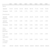
The share of the fund portfolio in each type of security is reported in Table 1. All funds in the sample are Spanish domestic equity funds. Therefore, as expected, the main investment is in domestic stocks. The CNMV requirements for this type of fund establish a minimum of 67% of the total portfolio invested in stocks issued in Spain, which is observable in most of the years reported in Table 1.
Portfolio holdings of Spanish domestic equity funds.
| 1999 | 2000 | 2001 | 2002 | 2003 | 2004 | 2005 | 2006 | |
| Stocks | ||||||||
| Spanish | 70.2% | 63.5% | 62.4% | 66.8% | 66.5% | 72.1% | 74.0% | 76.8% |
| European | 3.0% | 3.2% | 2.0% | 2.7% | 2.4% | 2.3% | 2.3% | 2.3% |
| Fixed income | ||||||||
| Spanish long-term | 10.9% | 15.4% | 19.6% | 12.4% | 20.4% | 18.2% | 15.6% | 14.4% |
| Spanish short-term | 4.5% | 5.3% | 3.6% | 3.8% | 2.4% | 1.8% | 2.1% | 1.0% |
| European | 0.0% | 0.0% | 0.0% | 0.0% | 0.4% | 0.0% | 0.3% | 0.0% |
| Other mutual fund units | 0.0% | 0.0% | 0.0% | 0.0% | 0.0% | 0.0% | 0.0% | 0.1% |
| Cash and cash equivalents | 8.0% | 8.9% | 9.7% | 12.2% | 7.4% | 5.1% | 5.4% | 4.9% |
| Non-controlled securities | 3.4% | 3.7% | 2.7% | 2.1% | 0.6% | 0.5% | 0.3% | 0.5% |
| Total | 100.0% | 100.0% | 100.0% | 100.0% | 100.0% | 100.0% | 100.0% | 100.0% |
This table reports the portfolio share by type of security for our sample. The assets invested by funds are classified by categories, as follows: stocks (Spanish and European), fixed income (Spanish long-term, Spanish short-term, and European), other mutual fund units, cash and cash equivalents, and non-controlled securities. The following data correspond to December of each year.
This section describes the methodology employed in this paper to determine whether a mutual fund engages in abnormal investment strategies around quarterly disclosures. Window-dressing practices have traditionally been tested by analyzing fund trading activity using portfolio holdings databases. Nevertheless, there is another approach that is based on the analysis of fund return anomalies around portfolio reporting dates. Meier and Schaumburg (2006) propose an approach that combines the use of both portfolio holdings and mutual fund returns. Taking advantage of the information that each database supplies, these authors propose a test to identify window-dressed portfolios by examining divergences between the return of the reported portfolio and the observed fund return. Interim fund trades cannot be directly captured with this approach. Nevertheless, an effort is made to solve this issue by performing a daily analysis of return differences. As a consequence, the assessment of fund management behaviour in between reporting dates can be improved. Moreover, this method has the advantage of analyzing each fund portfolio holding individually and not in an aggregate form, as is performed in other approaches employed to detect window-dressing practices.
4.1Return of the fund portfolio holdingsTo distinguish return patterns associated with potential window-dressing practices, the approach proposed by Meier and Schaumburg (2006) requires a benchmark to compare against the realized fund return. This benchmark is the return of the buy-and-hold strategy, which represents the return that the fund would have reached if the holdings of the disclosed portfolio were maintained for the period analyzed.
Given that window-dressing practices may imply higher trading activity just prior to reporting (Meier and Schaumburg, 2006; Elton et al., 2010), the analysis of return patterns is concentrated around mandatory reports. Meier and Schaumburg (2006) analyze US domestic equity funds that must report each quarter, but their database only covers semi-annual portfolio holdings. These authors then calculate the return on the buy-and-hold strategy in an interval that starts 91 days before the reporting date and ends 91 days afterwards (i.e., 13 weeks before and 13 weeks after), although they concentrate the analysis on the 4 weeks before and the 4 weeks after reporting.
In the Spanish market, mutual funds must report to investors quarterly, which would require a detailed analysis on a quarterly basis. However, our database of monthly portfolio holdings allows us to analyze every month. Therefore, our study overcomes the aforementioned study because it analyzes return patterns not only around disclosure portfolios (quarterly mandatory reports) but also around the non-disclosure portfolios. The return patterns associated with potential window-dressing practices are analyzed in an interval that starts one month before the reporting date and ends one month afterwards. The number of trading days varies depending on the month, with a maximum of 23 trading days. The interval analyzed can be defined between db and da, where db (da) is the number of trading days before (after) the reporting date.
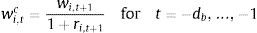
Each reported portfolio in our database shows the assets invested the last day of the month, so taking this day as t=0, the portfolio weight of each security i corresponds to reported security positions, as follows:
where Pi,t is the closing price of security i on day t,ni,t is the number of shares for security i on day t, and j is the total number of securities in the portfolio. As each reported portfolio shows the complete record of asset holdings and these securities are identified, the sum of all wi,t on day t=0 is 100%.
However, the portfolio weights calculated with Eq. (1) are only valid on the reporting day (t=0). Therefore, it is necessary to calculate the daily portfolio weight for the other days in the interval of interest (t=−db, …, da). As this weight calculation is performed under the assumption that funds follow a buy-and-hold strategy, the following process guarantees the correct daily updating of security positions according to their appreciation.
For any day after the reporting date (t=1, …, da), the portfolio weight of security i (wi,tc) is calculated from its weight on the previous day (wi,t−1) and the return on day t (ri,t). The daily security returns are calculated from datasets of daily closing prices, previously described in the data section.3 Then,

Note that to calculate the portfolio weights on day t=1, it is necessary to have the respective portfolio weights on day t=0, previously calculated and for which the sum of all wi,t=0 is 100%. Nevertheless, the sum of all wi,t=1c is different from 100%. For that reason, the final weights on day t=1 must be recalculated by a simple procedure that consists of finding the percentage that each wi,t=1c represent over the sum of all wi,t=1c. As a result, the sum of all final portfolio weights (wi,t) for day t=1 is 100%, and they can be employed as a base to calculate the portfolio weights on day t=2, and so on.
Following the above reasoning, for any day before the reporting date (t=−db, …, −1), the portfolio weight of security i (wi,tc) is calculated from its weight on the next day (wi,t+1) and the return obtained during day t+1 (ri,t+1), as:
Once again, the sum of all portfolio weights calculated for a day t (wi,tc) is different to 100%; therefore, they must be recalculated to obtain the final weights, which sum up to 100%.
Thus, once all final wi,t are obtained, the daily return of the fund portfolio holdings (Rk,tP) is computed for each reported portfolio by fund k and for each trading day t (t=−db, …, da), as follows:
where wi,t−1 is the weight that security i had on day t−1,ri,t is the return of security i on day t, and j is the total of securities in the portfolio.4.2Observed fund return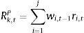
From the database of daily net asset values (NAV), the daily observed fund return is calculated for each fund as the relative change in NAV. However, the NAV return cannot be compared with the return of the fund portfolio holdings. The NAV return is net of the operating expenses, while the return of fund holdings does not include the subtraction corresponding to these expenses. To solve this incompatibility, the management fees are added back to the net fund return to obtain the gross fund return.
Daily returns are calculated for each fund over the period from December 1, 1999 through January 31, 2007. Therefore, a fund that exists throughout the sample period has 1,800 daily returns. For the entire sample of funds, a total of 177,792 daily fund returns are calculated.
4.3Return difference measureAs mentioned above, the key to identifying window-dressed portfolios is to analyze possible significant divergences between the daily return of fund portfolio holdings (Rk,tP) and the daily observed fund return (Rk,tF). These returns are calculated for each fund and each reported portfolio for a period of time spanning from a month before to a month after the reporting date (i.e., for t=−db, …, da). Following the approach of Meier and Schaumburg (2006), the return difference (RD) between these returns for fund k on day t is calculated as:
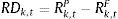
The analysis of the RD sign (i.e., positive or negative) is relevant to identify return patterns associated with portfolio manipulation practices. A significant positive RD implies that the buy-and-hold return of the reported portfolio outperforms the observed fund return. If this pattern occurs prior to the reporting date, it could indicate that the fund manipulates the portfolio by buying recently winner stocks and eliminating loser stocks. This window-dressing strategy results in a return of reported assets that is not representative of the portfolio held by the fund during the month, with the consequent difference in returns.
The window-dressing hypothesis states that fund managers are only motivated to improve the portfolio's image when they must disclose their portfolio holdings to clients. Therefore, one would expect that this trading strategy only appears before mandatory reports, which are reported quarterly for the Spanish market. This hypothesis can be verified in this study because our monthly database of portfolio holdings allows for the comparison of return patterns between disclosed and non-disclosed portfolios. Specifically, we expect to find a higher daily RD before the reporting dates for portfolios reported quarterly than for those in other months.
4.4Model specificationTo identify possible RD patterns associated with window-dressing practices, a detailed analysis of the RDs of each fund reported portfolio is conducted. Taking into account that a time series of RD is created for each reported portfolio, the RD study is based on a time series analysis of daily returns. These series elapse from db days before to da days after the reporting date.
Regarding the methodologies for a time series analysis, several financial studies employ linear regression models (OLS), assuming that the data are normally distributed, serial uncorrelated, and with constant variance. However, these assumptions are unrealistic to model some financial market variables. In particular, for financial market returns, the changes in variance over time have been widely documented.4 Therefore, models such as the Autoregressive Conditional Heteroscedastic (ARCH), introduced by Engle (1982), and the Generalized ARCH (GARCH), introduced by Bollerslev (1986), were developed to model changes in volatility.
The specification of a GARCH(p,q) model is given by the following equations:

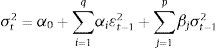
The equation of the mean (6) is written as a function of exogenous variables with an error term, while the variance Eq. (7) is written as a function of a constant, an ARCH, and a GARCH term. In the simplest form of GARCH models (i.e., the GARCH(1,1)), the variance equation is expressed as:
where the ARCH term (εt−12) contains information about volatility observed in the previous period, while the GARCH term (σt−12) contains information about the forecasted variance of the previous period.
The GARCH process defined by Bollerslev (1986) assumes that the conditional distribution of the error term (¿) is normal. However, the Student's t-distribution and the Generalized Error Distribution (GED) are widely employed. Independent of the distribution assumption, the GARCH models are typically estimated by the method of maximum likelihood.
Although the aim of this paper is to study the mean behaviour of the sample of the time series, the GARCH approach is employed to correct possible variance problems, such as heteroscedasticity and autocorrelation.
To determine the order of the GARCH model, some p, q combinations are applied to find the most accurate model for our sample. The results obtained suggest that the best model is the GARCH(1,1), which is in accordance with Bollerslev et al. (1986), who explain that the simple GARCH(1,1) model provides a good description of the data in most empirical applications. Once the order for the model has been specified, we find that the most accurate conditional distribution of the error term is the GED distribution. An advantage of the GED assumption is that it contains the normal distribution as a special case but also allows fatter and thinner tails than the ones in the normal distribution (Nelson, 1991). In summary, the time series analysis of the RDs will be performed by means of the GARCH(1,1) model, under the assumption that the errors follow a GED distribution.
5Identifying significant return differencesThis section focuses on the identification of filings where the reported portfolio is not informative of the actual return obtained by the fund. Once these portfolios are identified, we aim to provide evidence on two issues: first, to determine potential persistence in window-dresser funds; and second, to determine potential common characteristics in portfolios that have been manipulated. As previously mentioned, this study only focuses on the analysis of the mean to identify significant RDs and possible fund patterns. Given that the main goal is the identification of window-dressed portfolios, it is necessary to modify the mean equation (6) to differentiate the RD patterns before and after the reporting date because this phenomenon is mainly observed prior to reporting (Meier and Schaumburg, 2006; Elton et al., 2010). Therefore, the GARCH(1,1) model is specified with the following mean and variance equations:
where the equation of the mean (9) is written as a function of two dummy variables: BEFt and AFTt. BEFt takes the value of one for days before the reporting date and zero otherwise. In contrast, AFTt takes the value of one for days after the reporting date and zero otherwise. Note that in this equation, the t-test for β1 (β2) gives information about whether BEFt (AFTt) is significantly different from zero. Therefore, the estimation of this GARCH(1,1) model in each of the 6914 time series allows for the identification of portfolios with significant and positive RD before the reporting date, which are denominated hereafter as “identified portfolios”.

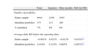
After the estimation process, 477 reported portfolios with a significantly positive BEFt coefficient (at 5% level) are found, which corresponds to 7% of the sample. The results are reported in Table 2. The average daily RD is significantly different (at the 1% level) between the entire sample and identified portfolios: −0.001% per day in the month leading up to the reporting date for the entire sample, and 0.104% for identified portfolios (Table 1).
Summary results for identified portfolios.
| Total | Quarters | Other months | Diff (Q,OM) | |
| Number of portfolios | ||||
| Entire sample | 6914 | 2359 | 4555 | |
| Identified portfolios | 477 | 213 | 264 | |
| % identified | 7% | 9% | 6% | |
| Average daily RD before the reporting date: | ||||
| Entire sample | −0.001% | 0.021% | −0.012% | 0.033%** |
| Identified portfolios | 0.104% | 0.152% | 0.065% | 0.087%** |
This table shows the number of portfolios and the average daily RD before the reporting date for the entire sample and the set of portfolios identified with a significant and positive BEFt coefficient from the GARCH estimation (Eqs. (9) and (10)). This information is also presented for months that coincide with mandatory disclosure dates (quarters) and other months. Moreover, the difference of the average daily RD between quarters (Q) and other months (OM) is reported in the final column.
This table also shows remarkable results when splitting the sample between months in which portfolios were disclosed (quarters) and other months. This classification reveals an interesting pattern consisting in that average daily RD is higher in portfolios reported on quarter-ends than in portfolios reported in other months, with differences statistically significant at a level of 1% for both the entire sample and the set of identified portfolios. This finding suggests that the main divergence between the return of the fund portfolio holdings and the observed fund return occurs prior to mandatory reports, which supports the window-dressing hypothesis. As expected under this hypothesis, identified portfolios reported on quarter-ends exhibit the highest average daily RD (0.152%). This result means that these mutual funds would have earned, on average, 0.152% more per day if they would have held the disclosed portfolio prior to the reporting date. This RD is even larger in our study than in Meier and Schaumburg's (2006) study; these authors find that the median return difference is approximately 0.05% per day in their sample of US mutual funds.
Fig. 1 uses box plots to better illustrate the RD behaviour for identified portfolios and their difference from the entire sample. For the entire sample (Panel A), the median is always near zero and the interquartile range before the reporting date ranges from −0.24% to 0.24%. The results for identified portfolios (Panel B) again show that the buy-and-hold return of the reported portfolio outperforms the observed fund return, especially prior to the reporting date, where the daily RD ranges from −0.40% to 0.44% and is in accordance with the expected portfolio manipulation pattern.
 and ending da days afterwards. The estimation of the GARCH(1,1) model (Eqs. (9) and (10)) allows for the identification of a set of reported portfolios with significant and positive BEFt coefficient. This figure shows the average daily RD for the entire sample (Panel A) and identified portfolios (Panel B). The boxes represent the interquartile range (i.e., the 25th and 75th percentile) and the line drawn across the boxes represents the median. The sample consists of 6,914 reported portfolios in Panel A and 477 in Panel B. portfolios.")
Pattern of daily RD for the entire sample and identified. For each reported portfolio, a time series of RD is created, starting db days before the reporting date (t=0) and ending da days afterwards. The estimation of the GARCH(1,1) model (Eqs. (9) and (10)) allows for the identification of a set of reported portfolios with significant and positive BEFt coefficient. This figure shows the average daily RD for the entire sample (Panel A) and identified portfolios (Panel B). The boxes represent the interquartile range (i.e., the 25th and 75th percentile) and the line drawn across the boxes represents the median. The sample consists of 6,914 reported portfolios in Panel A and 477 in Panel B. portfolios.
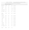
Portfolios that have been identified in the previous section have positive and significant RDs before the reporting dates; however, this condition is not enough to ensure that such portfolios have been manipulated according to window-dressing strategies. The window-dressing hypothesis states that fund managers are motivated to improve the portfolio's image when they must disclose their portfolio holdings to shareholders and clients. Therefore, one would expect this trading strategy to appear only near mandatory reports. The goal of this section is to analyze in detail the identified portfolios to determine whether fund managers follow certain cosmetic practices around portfolio disclosure to investors. Table 3 summarizes the main results related to the identified portfolios (by month).
Average daily RD for identified portfolios.
| Number of portfolios | Average daily RD for identified portfolios before the reporting date | |||
| Reported | Identified | % | ||
| Quarters | 2359 | 213 | 9% | 0.152% |
| March | 563 | 40 | 7% | 0.061% |
| June | 573 | 79 | 14% | 0.243% |
| September | 576 | 56 | 10% | 0.135% |
| December | 647 | 38 | 6% | 0.081% |
| Other months | 4555 | 264 | 6% | 0.065% |
| January | 558 | 36 | 6% | 0.057% |
| February | 563 | 33 | 6% | 0.082% |
| April | 565 | 30 | 5% | 0.094% |
| May | 568 | 46 | 8% | 0.064% |
| July | 572 | 41 | 7% | 0.057% |
| August | 576 | 28 | 5% | 0.038% |
| October | 577 | 27 | 5% | 0.068% |
| November | 576 | 23 | 4% | 0.061% |
| Total | 6914 | 477 | 7% | |
This table reports the main results of portfolios identified with significant and positive BEFt coefficients from the GARCH estimation (Eqs. (9) and (10)). By months, this table shows the number of portfolios reported and identified as well as the percentage of identified portfolios with respect to the sample. In addition, the average daily RD for identified portfolios before the reporting date is presented.
With regard to the number of portfolios, this table shows that June and September are the months with the highest percentage of identified portfolios with respect to the total number of reported portfolios in the sample (14% and 10% respectively). Moreover, when the average daily RD before the reporting date is analyzed, Table 3 reveals that the highest RD also corresponds to portfolios reported in June and September. In the previous section, Table 2 showed significant differences in daily RD of identified portfolios between quarter-end months and other months. Table 3 confirms former results and further details that the phenomenon is mostly driven by second and third quarter (June and September). The portfolio image at mid-year seems to be important in the Spanish industry compared to previous studies in which December is the month with higher window dressing activity. Note, however, that the frequency of our data allows us to deep in detail in other quarters rather than only the last one.
This differential pattern is better illustrated in Fig. 2. The comparison of the daily RD for portfolios that coincide with mandatory reports (Panel A) with those in other months (Panel B), reveals that something atypical occurs in quarterly reports. Before the reporting date, portfolios in Panel B exhibit a smaller dispersion and a median close to zero, while portfolios in Panel A show a positive RD, positive interquartile ranges, and a median of 0.08%. However, the RD behaviour for portfolios in June and September (Panels C and D) is even more remarkable because they display more positive interquartile ranges than the entire set of quarterly portfolios, and their median RD before the reporting date is approximately 0.20% and 0.06%, respectively (Fig. 1).
 and ending da days afterwards. The estimation of the GARCH(1,1) model (Eqs. (9) and (10)) allows for the identification of a set of reported portfolios with significant and positive BEFt coefficients. This figure illustrates the average daily RD for identified portfolios corresponding to quarterly mandatory reports (Panel A) and those in other months (Panel B). Moreover, Panels C and D show RD patterns in months with the highest percentage of identified portfolios with respect to the sample, June and September. The boxes represent the interquartile range (i.e., the 25th and 75th percentile) and the line drawn across the boxes represents the median. The sample consists of 213 portfolios in Panel A, 264 in Panel B, 79 in Panel C, and 56 in Panel D. portfolios.")
Pattern of daily RD for identified. For each reported portfolio, a time series of RD is created, starting db days before the reporting date (t=0) and ending da days afterwards. The estimation of the GARCH(1,1) model (Eqs. (9) and (10)) allows for the identification of a set of reported portfolios with significant and positive BEFt coefficients. This figure illustrates the average daily RD for identified portfolios corresponding to quarterly mandatory reports (Panel A) and those in other months (Panel B). Moreover, Panels C and D show RD patterns in months with the highest percentage of identified portfolios with respect to the sample, June and September. The boxes represent the interquartile range (i.e., the 25th and 75th percentile) and the line drawn across the boxes represents the median. The sample consists of 213 portfolios in Panel A, 264 in Panel B, 79 in Panel C, and 56 in Panel D. portfolios.
Regarding RD behaviour after the reporting date for quarterly portfolios, Fig. 2 shows that the average daily RD does not show a clear pattern; some days this difference is quite positive, while others it is very negative. This finding differs from the results obtained by Meier and Schaumburg (2006); they found no abnormal return differences after the reporting date, suggesting that the mutual funds might hold the reported portfolio over the next quarter. However, our results do not support this conclusion for the Spanish mutual funds, especially in June. This month funds exhibit significantly high turnover ratio which might explain those results.5
5.2Characteristics of window-dressed portfoliosThis section looks for potential common features in the portfolios that have been identified as window-dressed portfolios. Although the analysis only focuses on 213 portfolios, one might expect certain characteristics from funds that have manipulated their portfolios. For example, one would expect some of the following patterns: funds periodically window dress their portfolios; fund management companies follow window-dressing strategies in several funds that they manage; higher levels of window dressing occur in funds with poor past performance; and some coincidences in dates, among others.
In a first review of common characteristics in the sub-sample, we find that window-dressed portfolios are quite dispersed over funds, as 95 out of 125 funds in the sample have at least one portfolio identified as window dressed. In addition, the analysis of fund management companies for those funds with a higher percentage of window-dressed portfolios also shows a high dispersion level because a different company managed each fund.6
Regarding the dates of the identified portfolios, we find that each of the quarters of the sample period (29 in total) has at least one window-dressed portfolio. However, it is important to note that these portfolios are clustered over time, as about 40% correspond to three quarters in 2002 (specifically, June, September, and December). This fact is more interesting when it is related with the Ibex-35 performance on those dates because these were the months of the lowest profitability during the sample period.7 Therefore, these results might suggest that several funds found enough motivation to window dress their mandatory reports at the end of these bear market months, probably selling poor performing assets and buying recent winners to show high-quality portfolios at the end of the quarter. Although our finding contradicts the results of Meier and Schaumburg (2006), because they find that the use of window-dressing strategies is more likely in a bull market, it seems more reasonable to think that mutual funds need to engage in this type of strategies in poor performance periods, since they need to ensure that their clients are satisfied with the fund management.
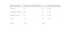
Finally, when funds are ranked by their past performance on the month before disclosure, the results in Table 4 show that 65% of the funds that manipulate their mandatory reports belong to medium-loser and loser return quartiles. Moreover, these funds have the characteristic of having a negative return of about −7.0% during the month leading up to the reporting date. This result might suggest that funds with poor past performance are more likely to manipulate their portfolios that are presented to clients. This behaviour of mutual funds is reasonable if one considers that many investors guide their decisions according to recent performance records (Chevalier and Ellison, 1997; Sirri and Tufano, 1998) (Table 4).
Past performance of window-dressed portfolios.
| Return quartile | Number of wd portfolios | % | Average fund return |
| Winner | 33 | 15 | −0.3% |
| Medium-Winner | 42 | 20 | −4.7% |
| Medium-Loser | 63 | 30 | −6.9% |
| Loser | 75 | 35 | −7.2% |
| Total | 213 | 100 | |
Each quarter, mutual funds are classified into four quartiles according to their cumulative return over the past month: Winner, Medium-Winner, Medium-Loser, and Loser. The Winner quartile contains the funds with the largest returns and the Loser quartile contains the funds with the smallest returns. This table reports, for each quartile, the number of window-dressed portfolios and the average fund return over the past month.
In summary, the analyses of identified portfolios that coincide with mandatory reports seem to indicate that the window-dressing practice is an isolated case within the sample of funds analyzed because these portfolios are distributed over funds and fund management companies. Nevertheless, the manipulated portfolios seem to be clustered over bear market periods, probably as a response to poor past performance.
6Summary and conclusionsSeveral studies have found evidence of the use of window-dressing practices by mutual funds by comparing portfolio holdings and analyzing their trading activity around disclosure dates. However, there are few studies in existing literature that analyze anomalies in mutual fund returns to identify these practices, and there is an even smaller number of studies that combine the analysis of observed fund returns with portfolio holdings information. In the latter subset, none of the studies use holdings data with a higher frequency than quarterly, which could limit their conclusions. Therefore, this paper aims to extend the study of portfolio manipulation around mandatory reports by examining daily observed fund returns and monthly portfolio holdings in Spain, a relevant European fund industry.
The detection of window-dressed portfolios is based on the analysis of the difference between the return of the reported fund holdings and the observed fund return. The estimation of a GARCH model allows for the identification of a low percentage of filings that have positive RD before the reporting date and that coincide with mandatory reports. The monthly database used allows for the comparison between disclosed and undisclosed identified portfolios, showing that the average daily RD is higher for quarterly portfolios than for those in other months. In addition, the results show that June and September are the months with the highest percentage of portfolios identified with respect to the total number of reported portfolios in the sample. The results also show that these portfolios have the highest RD before the reporting date. This finding is in accordance with expected results under the window-dressing hypothesis because those months coincide with mandatory reports.
The analyses of those portfolios identified as window-dressed portfolios suggest that window dressing is not a common practice in the Spanish equity funds. This conclusion is supported by the lesser proportion of filings identified in the extensive sample of portfolio holdings and the dispersion of these portfolios over funds and fund management companies. However, the results also suggest that funds with poor past performance are more likely to manipulate their portfolios and that window-dressed portfolios seem to be clustered over bear market periods, probably as a response to poor past performance.
The authors thank the UCEIF Foundation, research project ECO2009-12819-C03-02 of the Spanish Department of Science, and research project 268-159 of the University of Zaragoza for their financial support. We appreciate insightful comments from Miguel Ángel Martínez Sedano, Manuel Armada, Luis Vicente, and the participants of the XIX Finance Forum 2011 in Granada. Any possible errors in this article are the exclusive responsibility of the authors.
Law 35/2003, of November 4, on Collective Investment Schemes, establishes that managers must present a quarterly report for investors that includes, among other things, the portfolio composition of the fund.
The CNMV establishes in the CNMV Circular 1/2009, of February 4, that domestic equity funds are those that invest more than 75% of the portfolio in equities listed in Spanish stock exchange markets, including assets from Spanish issuers listed in other markets. The investment in stocks issued in Spain must be at least 90% of the equity portfolio, that is, at least 67% of the total portfolio. In addition, assets must be denominated in Euros, with a 30% limit in a non-Euro currency.
Returns for Spanish stocks are adjusted by dividends, stock splits, and seasoned equity offerings, while returns for European stocks are adjusted by dividends and stock splits.
See, for example, Fama (1965) and Lau et al. (1990).
We estimate the monthly portfolio turnover to explore the intensity of mutual fund trading throughout the calendar year. The results show that January, March and June are the months where the turnover ratio is significantly higher to the 12-month average ratio, at 1%significance level. These results are omitted for the sake of brevity, but this information is available upon request.
Tables with this information are not presented to avoid having large amounts of data without a significant contribution to the value of the analysis.
The monthly returns of Ibex-35 in June, September, and December 2002 were −13.04%, −15.60%, and −9.70%, respectively.

