


The goal of this article is to specify the role of financial analysts’ consensus in stock markets, specifically, the Eurostoxx Market, from January 2002 to December 2009. Financial analysts issue reports about companies quoted on the stock market. For each company and for a given time period, each report contains an estimate of its future earnings per share and dividends, its target price for the next twelve months and an investment recommendation such as ‘buy’, ‘sell’, or ‘hold’. Some firms collect these reports to calculate financial analysts’ consensus estimates. This article concludes that financial analysts’ consensus perform several functions: announcing in advance unexpected price changes (‘surprises’) through the target price, confirming previous estimations through revisions, and reflecting analysts’ convictions through the interpretation of their estimates. This role is modest but statistically significant in this market.
Financial analysts have been criticized for several reasons, especially in times of stock market and financial crisis: optimism bias in their estimates, weakened objectivity due to conflicts of interest, unrealistic target prices and passive monitoring of the market.
Despite these criticisms, the estimates of analysts are still used by many market participants, while financial data companies produce analyst consensus forecasts principally for investors. The consensus forecast is an average (i.e., median, in the case of the consensus provided by FactSet). It is assumed that the information value of the consensus forecast is known by all market participants and should already be incorporated into the security market price. If this is the case, then consensus does not affect the stock market price according to the Efficient Market Hypothesis and is information which will be of no value to the participants, supporting criticisms of analysts’ reports.
This article demonstrates that information in the consensus forecast is still useful for market participants even after 100 days, though the influence of this information is modest. To demonstrate this, three components of analysts’ reports are analyzed: estimated earnings, target prices and recommendations. Once the influence and informational content of these components have been assessed, a definition of the role of consensus among financial analysts is proposed.
The first section reviews previous research on financial analysts. The second section describes the sample that is the basis for the empirical analysis. The third section presents our research design and describes the models employed. The fourth section discusses the development and results of these models. In the fifth section, the role of analyst consensus is inferred from our models. The final section discusses the results of this research.
2The influence of analysts in the financial literatureA financial analyst's primary task is to scrutinize the financial condition of a company, assessing such characteristics as profitability, liquidity, and risk. This assessment is then presented in a report that contains earnings estimates, a target price that the analyst predicts the company's share price will attain within the next twelve months and a recommendation to investors to buy, sell or hold securities in the company.
Financial analysts may work in brokerage and securities companies that offer advisory and management services for the buying and selling of securities (sell-side analysts), in large investment institutions such as mutual funds or insurance companies (buy-side analysts) or as external professionals who advise several companies (independent analysts).
Given the internal use of buy-side analysts’ reports, this article will focus on both sell-side and independent analysts. Among these analysts, the article will focus on securities analysts and their role in the stock markets.
Three articles in recent decades have collected the results of academic research on financial analysts’ estimates and their influence on capital markets (Schipper, 1991; Brown, 1993; Ramnath et al., 2008). In these articles, it is clear that most research into the influence of analysts in the markets focuses on one of the three main components of analysts’ reports, i.e., earnings estimates, target prices or recommendations.
Regarding earnings estimates, the financial literature has shown that such estimates are superior to the predictions of time series models (Fried and Givoly, 1982; Brown et al., 1987; Wiedman, 1996). However, the information content has been found to lie in revisions of analysts’ earnings estimates of analysts rather than in the estimates themselves (Gleason and Lee, 2003; Aiolfi et al., 2010).
With respect to target prices, some studies show that they have more information content than recommendations, as target price is a more refined measure of company value (Da et al., 2008). Target prices have information value mainly in their revisions, although they have only a modest effect on yields if transaction costs are included (Barber et al., 2001; Brav and Lehavy, 2003).
As regards recommendations, the financial literature has shown that revisions in recommendations provide more information value than the level of recommendations (Stickel, 1995; Womack, 1996; Barber et al., 2001; Jegadeesh et al., 2004; Wang, 2012), although there is no agreement about the sign of revisions that offers the greatest information value.
While many studies have focused on revisions of each of the three components of analysts’ reports separately, studies that jointly investigate revisions of all three components are scarce. Those studies that exist have focused mainly on the additional information content provided by revisions of each component together with the other two. In addition, they focus on the complementary information content provided by the combination of the revisions of two of the three components (Francis and Soffer, 1997; Brav and Lehavy, 2003) or of all three components (Asquith et al., 2005; Feldman et al., 2012).
2.1The analyst consensusThe studies cited above show the influence of analysts, viewed as individuals, in particular markets. Few studies have examined the influence of analysts when they are considered as a consensus in a given market.
Analyst consensus has generally been used in the financial literature as a benchmark to highlight the performance of a single analyst against the average performance of a group of analysts (Cooper et al., 2001; Frankel et al., 2006). The consensus then allows the investor to form an opinion about a specific analyst (Park and Stice, 2000; Hong et al., 2000; Jegadeesh and Kim, 2010).
Previous research on the influence of analyst consensus has shown that revisions in consensus recommendations have a modest impact on capital markets. If transaction costs are taken into account, then revisions of consensus recommendations do not help investors achieve additional returns (Jegadeesh et al., 2004). What, then, is the use of an analyst consensus? To date the financial literature has not answered this question.
The aim of this paper is to identify the utility of analyst consensus by analyzing its content and influence in a specific market, jointly considering revisions of the three components of analysts’ reports. Our goal is to define the role of financial consensus in financial markets.
In this article, the consensus analysts’ forecast provided by FactSet for a particular month is defined as the median of the broker forecasts made in the last 100 days prior to the end of that month. This method uses the latest techniques for consensus (Wieland, 2011; Jegadeesh and Kim, 2010).
3Sample description3.1MarketData sample is obtained from quoted companies listed in the Eurostoxx index. This index, created by Stoxx Limited, is a broad and liquid subset from the STOXX Europe 600 index. With a variable number of components, it represents the companies with a large, medium and small capitalization from the 12 Eurozone countries. The Eurozone has received special attention during over recent years, amongst other reasons because of the high level of volatility in financial markets, markets which affect other emerging economies as well as other developed economies.
FactSet collects data from brokers on a voluntary basis, so there is potential for selection bias. This bias cannot be eliminated, as a company may not be followed either by analysts who collaborate with FactSet or by analysts in general. The selection of companies has been carried out according to the availability of data for the whole period.
3.2Period and frequencyThe sample period is set according to the availability of data from the FactSet database. The objective is to obtain the largest possible number of variables for the largest possible number of companies in each market and for the longest possible time period. The sample period is set to obtain the maximum number of observations possible and to ensure that the sample is balanced.
The period analyzed runs for 96 months from January 2002 until December 2009. The period starts with the recovery from the stock market crisis caused by the bursting of the dot.com bubble and ends with the financial crisis that began in 2007 but whose greatest impact would not begin until 2008 and would continue into 2009. For this reason, the period has two sub-periods: the pre-crisis stage (2002–2007) and the crisis stage (2008–2009), as seen in the behavior of the EUROSTOXX-50 index, shown in Chart 1.
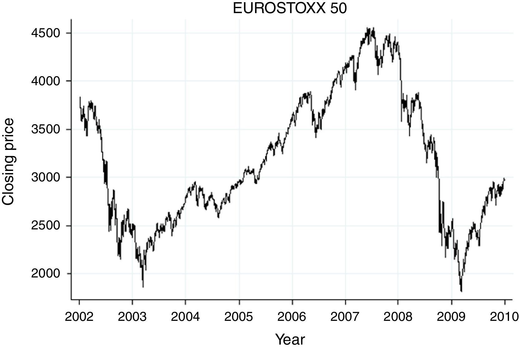
This division makes empirical analysis necessary both for the whole period and for each of the sub-periods. As it was a chain of events that led to the financial crisis, it is difficult to delimit the sub-periods; thus, delimitation was achieved by purely statistical means. Specifically, volatility was assessed and submitted to a Chow test to determine structural stability, as noted above.
Regarding data frequency, in most previous research, event time rather than calendar time has generally been used as a time reference, although articles combine both types (Ball and Bartov, 1995). Event time has the advantage of capturing the ability of analysts to detect market imperfections in setting prices in the light of available information about securities; thus, one can measure the short-term effect or the immediate impact of analysts’ estimates on the market. However, calendar time is actually easier for investors to use when they wish to establish strategies based on analysts’ recommendations. Thus, it is necessary to deepen the investigation of the influence of analysts on the market, using a calendar time reference, and for this reason, periodicity is monthly in this study, with data collected on the last day of each month. The window used by FactSet in the collection of this data is 100 days, which allows for the formation of a consensus based on more observations than that formed with data collected over a 45-day window.
3.3Sample data descriptionThe sample comprises 120 companies listed on the Eurostoxx index. As the analysis covers a 96-month period, the sample consists of 11,520 firm-month observations.
In this sample, 31 of the 120 companies belonged to the EUROSTOXX 50 on December 31, 2009, i.e., 25.83% of the companies in the sample. These 31 companies represent 76.83% of the total capitalization of the companies in the sample on that date.
The companies in the sample represent 57.95% of the capitalization of the Eurostoxx index on December 31, 2009. Those companies that belong to the EUROSTOXX 50 represent 68.72% of the capitalization of this index on that date. Sampled companies that belong to the EUROSTOXX Large, EUROSTOXX Mid and EUROSTOXX Small indexes, account for 62.25%, 38.16% and 35.35% of the capitalization of their corresponding indexes, respectively.
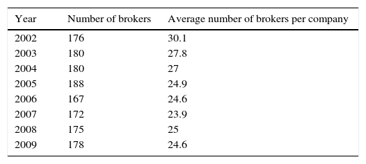
Consensus is not formed by a set of individual analysts but by a set of brokers that follow the evolution of securities prices in the stock market for the given 120 companies. Table 1 shows the average number of brokers that follow the securities prices of each company in the sample, along with the consensus figures.
4Methodology4.1The regression modelThis research requires the use of a dynamic panel data regression model (DPD), whose GMM estimator has the following characteristics:
- 1.
Difference-estimator: a difference-estimator is used, in view of the possibility that unobservable factors that change over time are correlated.
- 2.
Two-Step estimator: The relations among financial market participants are of a dynamic nature, and this is true in the case of financial analysts: they release their forecasts and these have an early impact on the markets, but after seeing these impacts they revise their forecasts again. This process has its statistical concretion in the presence of an endogenous lagged variable included among the explanatory variables. The two-step regressions are used to correct for possible endogeneity problems. In the first step, a model is estimated to try to explain the variable that causes endogeneity; this model is then used to estimate an endogeneity-free model.
- 3.
Robust estimator: Working with panel data of companies of different sizes, we are likely to find that the variability of large companies differs from that of small companies, giving rise to heteroskedasticity in the error terms (Wooldridge, 2006). To obviate possible heteroskedasticity in the errors, a robust estimator is used.
A model that meets these characteristics is the dynamic panel data (DPD) model proposed by Arellano and Bond (1991), whose general specification is as follows:
where δ denotes the intercept; i denotes the company i; i={1,…, N}; t denotes the month t; t={1,…, T}; l denotes the lag of the dependent variable, l={1,…, L}; k denotes the k explanatory variable; k={1,…, K}; αl is the coefficient of the dependent variable lagged l periods; xk,i,t is the observation of company i in the month t for the variable k; βk is the coefficient of explanatory variable k; μi indicates unobservable effects that differ between companies but not over time; εi,t indicates the coefficient of the random error term.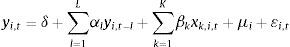
The Granger causality test (Granger, 1969) is applied to the model to ensure that the variable that captures the market reaction is statistically caused by these explanatory variables. The test for second-order serial correlation proposed by Arellano and Bond (1991) is also applied in order to verify the consistency of the estimators, as is the Sargan test (Sargan, 1964) for overidentifying restrictions in order to validate the use of additional instruments. The model also includes robust standard errors to take into account possible heteroskedasticity. The joint statistical significance of the estimated parameters test (Wald test) is also applied. Finally, supported by the Chow test, a model for each sub-period of the sample is statistically justified.
4.2Dependent variable that indicates the market reactionIn most models of market reactions to analysts’ forecasts, the dependent variable is the abnormal returns of companies studied by analysts. These returns are used to express exceptional variations in stock prices. Only in some models is the volatility the variable which is presumed to summarize the market effects of analysts’ reports (Athanassakos and Kalimipalli, 2004; Frankel et al., 2006; González and Gimeno, 2008; Schutte and Unlu, 2009). In this model, volatility is estimated as the dependent variable, capturing market reactions to financial analysts’ forecasts.
Time series of financial asset returns often exhibit the volatility clustering property: large changes in prices tend to cluster together, resulting in the persistence of the amplitudes of price changes, so that large variations in price (positive or negative) are expected after a large variation in price (of either sign), as noted by Mandelbrot (1963). A quantitative manifestation of this fact is that, while returns themselves are uncorrelated, the squared returns display a positive, significant and slowly decaying autocorrelation. This serial correlation in squared returns has been modeled by Bollerslev (1986) with the Generalized ARCH (GARCH) model.
Volatility is therefore calculated using the GARCH (1,1) model (Bollerslev, 1986), which works as an adaptive process that takes into account the conditioning variances at each stage so that clusters of high volatility can be grouped together.
4.3Explanatory variables related to analyst consensusThe research data contain financial analysts’ earnings estimates (and their revisions), target prices (and their revisions) and recommendations (and their revisions), provided by FactSet.
As noted above, prior investigations have recognized that analysts’ revisions of estimates have a greater influence on the market than initial estimates. Therefore, the explanatory variables in the models are revisions of earnings estimates, of target prices and of recommendations. For this reason, the data provided by FactSet are grouped around the following sets of variables:
- -
Revisions of earnings estimates. Number of revisions of consensus earnings per share in a month: upward revisions (eeps1revup and eeps2revup), downward revisions (eeps1revdwn and eeps2revdwn), and revisions that do not change earnings estimates (eeps1revunch and eeps2revunch) for the end of the current year and for the end of the following year. For example: Number of revisions of consensus earnings per share estimates available on 01/31/2002 for 12/31/2002 and 12/31/2003.
- -
Revisions of target prices. Number of upward revisions (tprevup), downward revisions (tprevdwn) and revisions in which target prices are unchanged (tprevunch).
- -
Revisions of recommendations. Number of upward revisions (reupward), downward revisions (redownward) and revisions in which the recommendation is unchanged (reunchanged). An upward revision of a recommendation occurs when there is change in the level of recommendation in the direction sell-hold-buy. A downward revision of a recommendation occurs when there is change in the level recommendation in the direction buy-hold-sell.
To ensure multicollinearity-free selection, the condition index is reported.
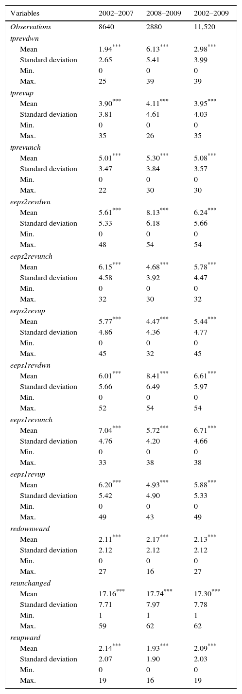
4.4Descriptive statisticsTable 2 shows the descriptive statistics of the explanatory variables:
Descriptive statistics.
| Variables | 2002–2007 | 2008–2009 | 2002–2009 |
|---|---|---|---|
| Observations | 8640 | 2880 | 11,520 |
| tprevdwn | |||
| Mean | 1.94*** | 6.13*** | 2.98*** |
| Standard deviation | 2.65 | 5.41 | 3.99 |
| Min. | 0 | 0 | 0 |
| Max. | 25 | 39 | 39 |
| tprevup | |||
| Mean | 3.90*** | 4.11*** | 3.95*** |
| Standard deviation | 3.81 | 4.61 | 4.03 |
| Min. | 0 | 0 | 0 |
| Max. | 35 | 26 | 35 |
| tprevunch | |||
| Mean | 5.01*** | 5.30*** | 5.08*** |
| Standard deviation | 3.47 | 3.84 | 3.57 |
| Min. | 0 | 0 | 0 |
| Max. | 22 | 30 | 30 |
| eeps2revdwn | |||
| Mean | 5.61*** | 8.13*** | 6.24*** |
| Standard deviation | 5.33 | 6.18 | 5.66 |
| Min. | 0 | 0 | 0 |
| Max. | 48 | 54 | 54 |
| eeps2revunch | |||
| Mean | 6.15*** | 4.68*** | 5.78*** |
| Standard deviation | 4.58 | 3.92 | 4.47 |
| Min. | 0 | 0 | 0 |
| Max. | 32 | 30 | 32 |
| eeps2revup | |||
| Mean | 5.77*** | 4.47*** | 5.44*** |
| Standard deviation | 4.86 | 4.36 | 4.77 |
| Min. | 0 | 0 | 0 |
| Max. | 45 | 32 | 45 |
| eeps1revdwn | |||
| Mean | 6.01*** | 8.41*** | 6.61*** |
| Standard deviation | 5.66 | 6.49 | 5.97 |
| Min. | 0 | 0 | 0 |
| Max. | 52 | 54 | 54 |
| eeps1revunch | |||
| Mean | 7.04*** | 5.72*** | 6.71*** |
| Standard deviation | 4.76 | 4.20 | 4.66 |
| Min. | 0 | 0 | 0 |
| Max. | 33 | 38 | 38 |
| eeps1revup | |||
| Mean | 6.20*** | 4.93*** | 5.88*** |
| Standard deviation | 5.42 | 4.90 | 5.33 |
| Min. | 0 | 0 | 0 |
| Max. | 49 | 43 | 49 |
| redownward | |||
| Mean | 2.11*** | 2.17*** | 2.13*** |
| Standard deviation | 2.12 | 2.12 | 2.12 |
| Min. | 0 | 0 | 0 |
| Max. | 27 | 16 | 27 |
| reunchanged | |||
| Mean | 17.16*** | 17.74*** | 17.30*** |
| Standard deviation | 7.71 | 7.97 | 7.78 |
| Min. | 1 | 1 | 1 |
| Max. | 59 | 62 | 62 |
| reupward | |||
| Mean | 2.14*** | 1.93*** | 2.09*** |
| Standard deviation | 2.07 | 1.90 | 2.03 |
| Min. | 0 | 0 | 0 |
| Max. | 19 | 16 | 19 |
This table provides descriptive statistics on the revisions of analyst consensus estimates. Variables: tprevdwn is the number of monthly downward revisions of consensus target price; tprevup is the number of monthly upward revisions of consensus target price; tprevunch is the number of monthly revisions in which target price remains unchanged; eeps2revdwn is the number of downward revisions of consensus earnings per share for the end of the following year; eeps2revunch is the number of monthly revisions that do not change consensus earnings estimates for the end of the following year; eeps2revup is the number of upward revisions of consensus earnings per share for the end of the following year; eeps1revdwn is the number of downward revisions of consensus earnings per share for the current year; eeps1revunch is the number of monthly revisions that do not change consensus earnings estimates for the current year; eeps1revup is the number of upward revisions of consensus earnings per share for the current year; redownward: number of monthly downward revisions of consensus recommendation (an downward revision of a recommendation occurs when there is a change in the level of recommendation in the direction buy-hold-sell); reunchanged: number of monthly revisions in which the recommendation is unchanged; reupward: number of monthly upward revisions of consensus recommendation (an upward revision of a recommendation occurs when there is a change in the level of recommendation in the direction sell-hold-buy).
Regarding revisions of expected earnings, it can be observed that, for the period 2008–2009, the average number of monthly downward revisions increased with respect to the average for the period 2002–2007. This was the result of the pessimistic perspectives arising from the financial crisis.
This explains that during the period 2008–2009, the average number of downward revisions of target prices increased. There is a significant change in 2008–2009 compared with 2002–2007: the average number of monthly downward revisions ranges from 1.94 to 6.13.
However the average number of downward revisions of the level of recommendations hardly varied from 2002–2007 to 2008–2009. In general, the average number of monthly revisions of the level of recommendations hardly varied from one period to another.
4.5Groups of modelsTo construct all the models and to avoid the problem of autocorrelation, it has been necessary to consider five lags of the dependent variable as independent variables in all models. This is because problems of autocorrelation arise when fewer lags are analyzed. Hence the volatility (LNVolatility) of the dependent variable is explained in each model by five lags of itself and by the selected variables that represent revisions of financial analysts’ consensus views.
We construct 6 groups of models:
- 1.
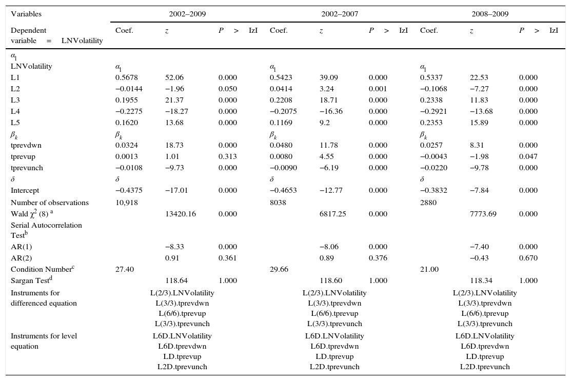
Models with target price revisions: These models are composed of the number of monthly revisions of consensus target price as explanatory variables.
- 2.
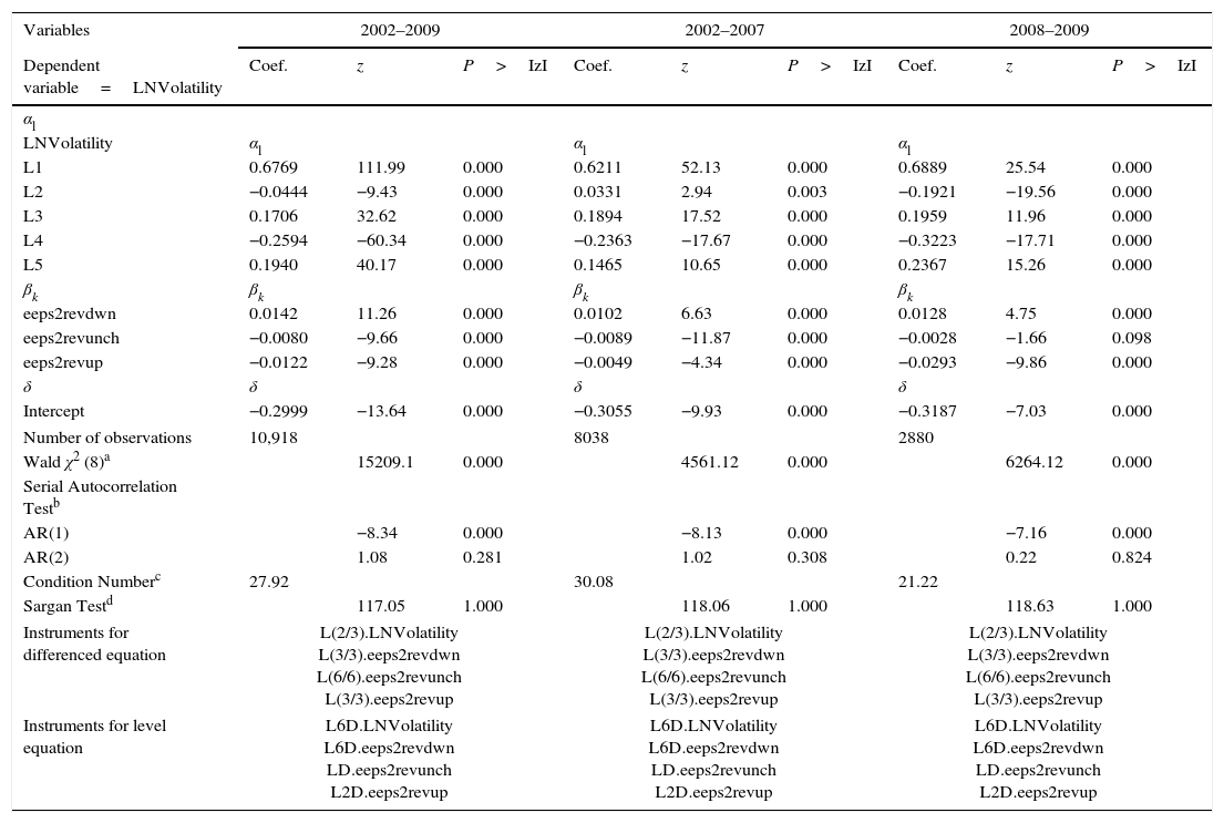
Models with estimated next-year EPS revisions: In these models, the explanatory variables are the number of monthly revisions of consensus earnings per share for the end of the following year.
- 3.
Models with estimated current-year EPS revisions: Here, the explanatory variables are the number of monthly revisions of consensus earnings per share for the end of the current year.
- 4.
Models with recommendations revisions: These models are composed of the number of monthly revisions of recommendations as explanatory variables.
- 5.
Models with significant variables: In these models, the explanatory variables are selected after constructing the models with all variables that represent revisions of financial analysts’ consensus and choosing those variables which are significant ones. These variables are the following: tprevdwn, eeps2revdwn and reupward.
- 6.
Models in line with previous research: In these models four criteria are used to select the three variables in the models:
- (i)
One variable from each set of the financial analyst's report, starting with the number of downward revisions of target prices.
- (ii)
A significant correlation with the dependent variable (LNVolatility).
- (iii)
The passing of the Granger test, to ensure statistical causality.
- (iv)
The lowest correlation with the other explanatory variables, to avoid multicollinearity.
In the light of these criteria, the explanatory variables selected as suitable for the models are the following: tprevdwn, eeps2revunch and reupward. This selection is in line with previous research.
- (i)
The annex shows the tables that list all these groups of models except the table for the chosen group.
4.6Choosing the group of modelsWe choose that group of models that captures the most significant effects of changes in analysts’ consensus revisions on volatility.
To see the effects of changes in analyst consensus on volatility, it is necessary to compare the residual errors of the models that include analysts’ estimates with the residual errors of those that do not include analysts’ estimates, i.e., models in which volatility in a given month is a function of volatility in the preceding months. This comparison yields the following results.
Residual errors reflect the portion of the variation in the dependent variable which is not explained by the independent variables. When the variables reflecting revisions of analyst consensus are included in the model, unexplained variations in the dependent variable are reduced. Thus, there is less uncertainty about the factors that influence changes in volatility in models that include analysts’ estimates than in those that do not. Such models therefore provide more information about the volatility of the markets and the factors involved the evolution of volatility.
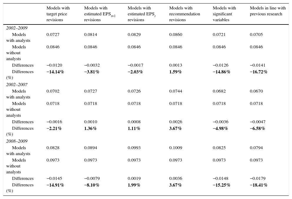
Table 3 shows that the explanatory power of variables that reflect analysts’ estimates increases significantly during the crisis sub-period. That is, investors pay more attention to analysts’ estimates in times of downward trending stock prices than in times of rising prices. In times of crisis, uncertainty evidently compels investors to seek more information on the forecasts of securities analysts.
Standard deviation of residuals.
| Models with target price revisions | Models with estimated EPSt+1 revisions | Models with estimated EPSt revisions | Models with recommendation revisions | Models with significant variables | Models in line with previous research | |
|---|---|---|---|---|---|---|
| 2002–2009 | ||||||
| Models with analysts | 0.0727 | 0.0814 | 0.0829 | 0.0860 | 0.0721 | 0.0705 |
| Models without analysts | 0.0846 | 0.0846 | 0.0846 | 0.0846 | 0.0846 | 0.0846 |
| Differences | −0.0120 | −0.0032 | −0.0017 | 0.0013 | −0.0126 | −0.0141 |
| Differences (%) | −14.14% | −3.81% | −2.03% | 1.59% | −14.86% | −16.72% |
| 2002–2007 | ||||||
| Models with analysts | 0.0702 | 0.0727 | 0.0726 | 0.0744 | 0.0682 | 0.0670 |
| Models without analysts | 0.0718 | 0.0718 | 0.0718 | 0.0718 | 0.0718 | 0.0718 |
| Differences | −0.0016 | 0.0010 | 0.0008 | 0.0026 | −0.0036 | −0.0047 |
| Differences (%) | −2.21% | 1.36% | 1.11% | 3.67% | −4.98% | −6.58% |
| 2008–2009 | ||||||
| Models with analysts | 0.0828 | 0.0894 | 0.0993 | 0.1009 | 0.0825 | 0.0794 |
| Models without analysts | 0.0973 | 0.0973 | 0.0973 | 0.0973 | 0.0973 | 0.0973 |
| Differences | −0.0145 | −0.0079 | 0.0019 | 0.0036 | −0.0148 | −0.0179 |
| Differences (%) | −14.91% | −8.10% | 1.99% | 3.67% | −15.25% | −18.41% |
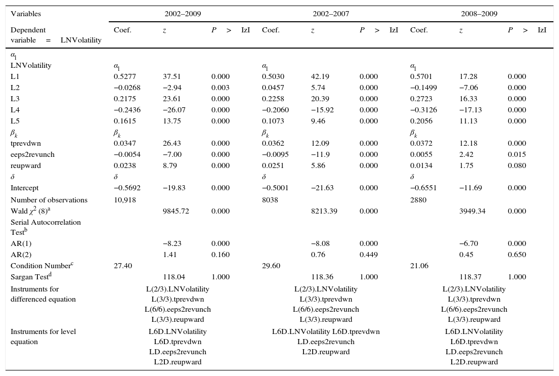
According to Table 3, among all groups the group of models in line with previous research provides more information about the volatility of the markets in all periods. This group has the lowest standard deviation of residuals in every period and reduces by 16.72% the unexplained variations in the dependent variable in 2002–2009. Table 4 lists this group of models:
Models in line with previous research.
| Variables | 2002–2009 | 2002–2007 | 2008–2009 | ||||||
|---|---|---|---|---|---|---|---|---|---|
| Dependent variable=LNVolatility | Coef. | z | P>IzI | Coef. | z | P>IzI | Coef. | z | P>IzI |
| αl | |||||||||
| LNVolatility | αl | αl | αl | ||||||
| L1 | 0.5277 | 37.51 | 0.000 | 0.5030 | 42.19 | 0.000 | 0.5701 | 17.28 | 0.000 |
| L2 | −0.0268 | −2.94 | 0.003 | 0.0457 | 5.74 | 0.000 | −0.1499 | −7.06 | 0.000 |
| L3 | 0.2175 | 23.61 | 0.000 | 0.2258 | 20.39 | 0.000 | 0.2723 | 16.33 | 0.000 |
| L4 | −0.2436 | −26.07 | 0.000 | −0.2060 | −15.92 | 0.000 | −0.3126 | −17.13 | 0.000 |
| L5 | 0.1615 | 13.75 | 0.000 | 0.1073 | 9.46 | 0.000 | 0.2056 | 11.13 | 0.000 |
| βk | βk | βk | βk | ||||||
| tprevdwn | 0.0347 | 26.43 | 0.000 | 0.0362 | 12.09 | 0.000 | 0.0372 | 12.18 | 0.000 |
| eeps2revunch | −0.0054 | −7.00 | 0.000 | −0.0095 | −11.9 | 0.000 | 0.0055 | 2.42 | 0.015 |
| reupward | 0.0238 | 8.79 | 0.000 | 0.0251 | 5.86 | 0.000 | 0.0134 | 1.75 | 0.080 |
| δ | δ | δ | δ | ||||||
| Intercept | −0.5692 | −19.83 | 0.000 | −0.5001 | −21.63 | 0.000 | −0.6551 | −11.69 | 0.000 |
| Number of observations | 10,918 | 8038 | 2880 | ||||||
| Wald χ2 (8)a | 9845.72 | 0.000 | 8213.39 | 0.000 | 3949.34 | 0.000 | |||
| Serial Autocorrelation Testb | |||||||||
| AR(1) | −8.23 | 0.000 | −8.08 | 0.000 | −6.70 | 0.000 | |||
| AR(2) | 1.41 | 0.160 | 0.76 | 0.449 | 0.45 | 0.650 | |||
| Condition Numberc | 27.40 | 29.60 | 21.06 | ||||||
| Sargan Testd | 118.04 | 1.000 | 118.36 | 1.000 | 118.37 | 1.000 | |||
| Instruments for differenced equation | L(2/3).LNVolatility L(3/3).tprevdwn L(6/6).eeps2revunch L(3/3).reupward | L(2/3).LNVolatility L(3/3).tprevdwn L(6/6).eeps2revunch L(3/3).reupward | L(2/3).LNVolatility L(3/3).tprevdwn L(6/6).eeps2revunch L(3/3).reupward | ||||||
| Instruments for level equation | L6D.LNVolatility L6D.tprevdwn LD.eeps2revunch L2D.reupward | L6D.LNVolatility L6D.tprevdwn LD.eeps2revunch L2D.reupward | L6D.LNVolatility L6D.tprevdwn LD.eeps2revunch L2D.reupward | ||||||
This table reports the result when volatility are regressed on various explanatory variables. LNVolatility is the monthly volatility and is estimated as the dependent variable, capturing market reactions to financial analysts’ consensus forecasts through a DPD model in differences and in two steps (Arellano and Bond, 1991). Monthly volatility is calculated using the GARCH (1,1) model (Bollerslev, 1986); LNVolatility L1, L2, L3, L4, and L5, are the monthly volatility lagged one, two, three, four, and five months; tprevdwn is the number of monthly downward revisions of consensus target price; eeps2revunch is the number of monthly revisions that do not change consensus earnings estimates for the end of the following year; reupward: number of monthly upward revisions of consensus recommendation (an upward revision of a recommendation occurs when there is a change in the level of recommendation in the direction sell-hold-buy).
This table offers the following observations: (1) all variables that represent revisions of financial analysts’ consensus views are significant in each model; this is the most significant result, in view of the purpose of this study; (2) all eight explanatory variables, viewed as a whole, are significant; (3) the three explanatory variables representing the consensus views of financial analysts, viewed collectively, are significant. In view of the resulting models (Table 4), it is worth noting the following:
- 1.
Volatility as measured in previous months influences volatility in the present month. The persistence of volatility is most significant in periods of crisis, a finding that appears logical, given that crises are periods of considerable uncertainty.
- 2.
The parameters indicating downward target price revisions (tprevdwn) increase in periods of crisis: revisions that lower the target price of companies increase when the expectations of their future earnings, of their sectors’ earnings and of European macroeconomic indicators, worsen.
- 3.
The parameters indicating revisions that modify expected EPS in the following year (eeps2revunch) always appear with negative signs: when the expected EPS for the following year does not change, there is uncertainty regarding the analyzed securities and thus their volatility is reduced.
- 4.
The strength and significance of the variable reupward (revisions that upgrade the level of a recommendation) both decline during periods of crisis. This finding appears logical, as expectations tend to worsen in periods of crisis.
The test of structural stability of the model (Chow test) is applied to check whether consideration of two sub-periods (a pre-crisis sub-period and a crisis sub-period) is warranted. This test is applied by using the data of each sub-period to form two samples and creating two variables from each explanatory variable: the variables that end in 1 refer to the pre-crisis sub-period; the variables that end in 2 refer to the crisis sub-period. A DPD model is then applied using all the variables, to check whether the coefficients of the variables that end in 1 match those that end in 2. The null hypothesis is that the coefficients match, i.e.:
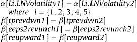
The test yields the following results
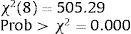
The coefficients of the variables of the pre-crisis sub-period do not match those of the variables of the crisis sub-period. Thus, a model for each sub-period is warranted.
5Contribution of the analyst consensusOnce the models presented in Table 4 are confirmed, we examine the influence of each variable on variations in volatility, in particular, the role of analyst consensus in the markets.
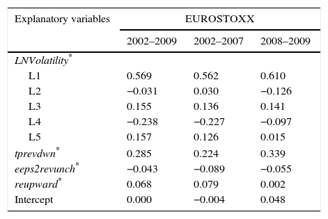
5.1The influence of the explanatory variables on volatilityIn order to quantify the effect of the explanatory variables on volatility, each variable is first standardized, and the models re-estimated. The variable coefficients are then compared. Table 5 shows the results.
Influence of the explanatory variables on volatility.
| Explanatory variables | EUROSTOXX | ||
|---|---|---|---|
| 2002–2009 | 2002–2007 | 2008–2009 | |
| LNVolatility* | |||
| L1 | 0.569 | 0.562 | 0.610 |
| L2 | −0.031 | 0.030 | −0.126 |
| L3 | 0.155 | 0.136 | 0.141 |
| L4 | −0.238 | −0.227 | −0.097 |
| L5 | 0.157 | 0.126 | 0.015 |
| tprevdwn* | 0.285 | 0.224 | 0.339 |
| eeps2revunch* | −0.043 | −0.089 | −0.055 |
| reupward* | 0.068 | 0.079 | 0.002 |
| Intercept | 0.000 | −0.004 | 0.048 |
This table reports the result when volatility are regressed on various explanatory variables. Explanatory variables are standarized in order to compare their contributions to volatility. LNVolatility L1, L2, L3, L4, and L5, are the monthly volatility lagged one, two, three, four, and five months and are calculated using the GARCH (1,1) model (Bollerslev, 1986); tprevdwn is the number of monthly downward revisions of consensus target price; eeps2revunch is the number of monthly revisions that do not change consensus earnings estimates for the end of the following year; reupward is number of monthly upward revisions of consensus recommendation (an upward revision of a recommendation occurs when there is a change in the level of recommendation in the direction sell-hold-buy).
It is evident that of the variables reflecting analyst consensus, that which corresponds to the number of downward revisions of the target price (tprevdwn) has the strongest influence (with respect to the absolute values) on volatility. This result is consistent with results of previous research: more information is obtained from estimates of target price than from estimates of a company's future earnings (estimates of future cash flows adjusted to risk), from estimates of future profitability of the industry to which that company belongs, or from assessments of macroeconomic factors that affect the market as a whole (Asquith et al., 2005; Bradshaw, 2002). This variable is also the second most influential in the entire model, the first being the previous month's volatility. During the crisis sub-period, the influence of downward revisions of target price on volatility strengthens. If investors are sensitive to downward revisions of target prices, this sensitivity increases considerably in periods of falling stock prices.
The next most influential variable (in absolute terms), among those reflecting analyst consensus, is the variable for revisions of earnings estimates where forecasts for the following year's EPS remain unchanged (eeps2revunch) (though this is not the case for the full period, 2002–2009). These revisions reduce volatility; thus, the coefficient has a negative sign in all models. This is as expected, as uncertainty about next year should exceed uncertainty about the current year; and if the revisions do not entail variation in estimated earnings, then uncertainty should decrease.
Finally, the least influential variable is upward revisions of recommendations (reupward). According to these models, investors pay more attention to target price and earnings estimates than to recommendations, although they do not altogether ignore the latter. This is consistent with the idea that the value of recommendations lies in the level of commitment of the analysts in providing their estimates; but the most interesting information for investors is evidently the estimates themselves.
5.2Contribution of the analyst consensus in stock marketsAfter showing the impact of each explanatory variable on volatility, the next step is to assess the implications of the variables with respect to the influence of analyst consensus on markets.
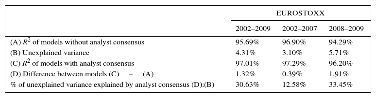
To determine the influence of analysts on variations in volatility, it is helpful to examine the coefficient of determination (R2) for both types of models, those that include the variables reflecting analyst estimates and those that do not. The coefficient of determination is defined as follows:
where Sres2, variance of residuals of the models; SLNVol2, variance of the dependent variable LNVolatility.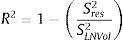
Without contextualizing their results, financial analyst consensus seem to add very little explanatory power. Models are intended to capture the idea that monthly volatility contains information about the last 120 days (not only from the analyst consensus, which is supposed to be fully known by all market participants, but also from the volatility that has taken place five months previously, i.e., approximately 120 days). Taking this into account, the unexplained variance must be close to 0. Information managed by analyst consensus through their revisions in the last 100 days has been thought to have no influence on the monthly volatility since it is assumed that such information has already been incorporated in stock prices. However, this is not the case as is illustrated in Table 6.
The coefficient of determination of the models.
| EUROSTOXX | |||
|---|---|---|---|
| 2002–2009 | 2002–2007 | 2008–2009 | |
| (A) R2 of models without analyst consensus | 95.69% | 96.90% | 94.29% |
| (B) Unexplained variance | 4.31% | 3.10% | 5.71% |
| (C) R2 of models with analyst consensus | 97.01% | 97.29% | 96.20% |
| (D) Difference between models (C)−(A) | 1.32% | 0.39% | 1.91% |
| % of unexplained variance explained by analyst consensus (D):(B) | 30.63% | 12.58% | 33.45% |
For the whole period, the 30.63% of the unexplained variance obtained by using only the models without analysts is explained by analysts. This percentage increases during the crisis period. Something happens in the financial markets that causes some public information to take a long time to be incorporated into financial assets prices. From this perspective, I would not consider the explanatory power added by analysts to be small.
6Comments on the resultsThe influence of analyst consensus on market volatility is modest. Though modest, this contribution is significant, suggesting that other possible factors in market movements—factors not specified in the model—are less significant.
The financial literature has confirmed the optimism bias of financial analysts in their forecasts. If investors are aware of this bias, then they will expect that any revision made by analysts will be likely to be upward rather than downward. For this reason, it is usually expected that downward revisions will convey unexpected information and involve a significant reaction from investors. The models in Table 4 show that downward revisions of target prices significantly influence the market by increasing volatility.
Target prices are arrived at by taking into account, amongst other things, estimates of earnings. Consequently, a common expectation is that downward revisions will exert more influence on the market than upward revisions. Table 5 confirms this expectation: among the variables that represent analysts’ consensus, downward revisions of target prices exert the strongest influence on volatility.
Analysts can revise any of three groups of estimates: target prices, future earnings, and recommendations. All the studies of the role of financial analysts to date, however, have focused on only one or two of these groups (for example, on the future earnings and/or on recommendations). The present empirical analysis demonstrates that the three groups of information simultaneously influence volatility since each group of estimates provides marginal information not captured by the other groups. This general model thus describes the following functions that together define the role of the securities analysts’ consensus:
- (a)
Revisions of target price and the element of surprise
In line with previous financial literature, the consensus of financial analysts is seen to be affected by individual analysts’ optimism bias (Brav and Lehavy, 2003; Cowen et al., 2006; Kerl and Walter, 2008). As shown in the literature, this persistence of optimism bias is known about by the market participants. Therefore, revisions of the consensus target price that push the consensus in a direction contrary to the one indicated by the optimism of analysts have a stronger impact on markets than upward revisions. Investors know that when analysts move the target price downward after its revision, it means that unexpected information has appeared.
Thus, downward revisions of target prices capture the element of surprise, i.e., the unexpected factor in the future development of the company. This element of surprise produces an upward variation in volatility.
- (b)
Revisions of estimated future earnings and the Confirmation Factor
Through revisions, analysts update their estimates with new information. When revisions leave the expected EPS for the following year intact, the degree of uncertainty is reduced and the new information that prompts analysts to revise their estimates confirms those estimates. Consequently, analysts as a whole provide a “confirming factor” to investors through the revisions of estimated future earnings.
- (c)
Revisions of the analysts’ recommendations and the Commitment Factor
Analysts’ recommendations also exert an influence, although to a lesser extent than the other two components of the analyst's report. This is explained by the fact that the same recommendation issued by one analyst does not produce the same reaction on the part of all investors, even if the analyst enjoys the same reputation among all investors. This is not unusual since each investor is not starting from exactly the same position in the market, i.e., each portfolio does not have the same asset allocation. As a result, the effect of a specific recommendation (or of a revision that modifies a specific recommendation) will depend, among other factors, on the asset allocation of each investor at the time the analysts recommended to buy, sell or hold certain securities.
It thus makes sense to consider the value of the analyst's recommendation, together with the other two components of her (his) reports. As the financial literature already shows, when an analyst offers a recommendation after making her (his) estimates, she (he) is offering an interpretation of these estimates. Thus the analyst, through interpretation, commits herself (himself) to her (his) estimates.
It is logical to expect that revisions that upgrade the level of recommendation convey this commitment factor. These revisions produce an increase in on volatility because they encourage investors to make changes toward long positions with the recommended stock, encouraging its trading. It is therefore the case that analyst consensus affects the stock market price though in a modest way.
Future research might involve the repetition of this analysis for other markets (US markets, emerging markets) and with data from other sources (Reuters, IBES) in order to compare results.
Models with target price revisions.
| Variables | 2002–2009 | 2002–2007 | 2008–2009 | ||||||
|---|---|---|---|---|---|---|---|---|---|
| Dependent variable=LNVolatility | Coef. | z | P>IzI | Coef. | z | P>IzI | Coef. | z | P>IzI |
| αl | |||||||||
| LNVolatility | αl | αl | αl | ||||||
| L1 | 0.5678 | 52.06 | 0.000 | 0.5423 | 39.09 | 0.000 | 0.5337 | 22.53 | 0.000 |
| L2 | −0.0144 | −1.96 | 0.050 | 0.0414 | 3.24 | 0.001 | −0.1068 | −7.27 | 0.000 |
| L3 | 0.1955 | 21.37 | 0.000 | 0.2208 | 18.71 | 0.000 | 0.2338 | 11.83 | 0.000 |
| L4 | −0.2275 | −18.27 | 0.000 | −0.2075 | −16.36 | 0.000 | −0.2921 | −13.68 | 0.000 |
| L5 | 0.1620 | 13.68 | 0.000 | 0.1169 | 9.2 | 0.000 | 0.2353 | 15.89 | 0.000 |
| βk | βk | βk | βk | ||||||
| tprevdwn | 0.0324 | 18.73 | 0.000 | 0.0480 | 11.78 | 0.000 | 0.0257 | 8.31 | 0.000 |
| tprevup | 0.0013 | 1.01 | 0.313 | 0.0080 | 4.55 | 0.000 | −0.0043 | −1.98 | 0.047 |
| tprevunch | −0.0108 | −9.73 | 0.000 | −0.0090 | −6.19 | 0.000 | −0.0220 | −9.78 | 0.000 |
| δ | δ | δ | δ | ||||||
| Intercept | −0.4375 | −17.01 | 0.000 | −0.4653 | −12.77 | 0.000 | −0.3832 | −7.84 | 0.000 |
| Number of observations | 10,918 | 8038 | 2880 | ||||||
| Wald χ2 (8) a | 13420.16 | 0.000 | 6817.25 | 0.000 | 7773.69 | 0.000 | |||
| Serial Autocorrelation Testb | |||||||||
| AR(1) | −8.33 | 0.000 | −8.06 | 0.000 | −7.40 | 0.000 | |||
| AR(2) | 0.91 | 0.361 | 0.89 | 0.376 | −0.43 | 0.670 | |||
| Condition Numberc | 27.40 | 29.66 | 21.00 | ||||||
| Sargan Testd | 118.64 | 1.000 | 118.60 | 1.000 | 118.34 | 1.000 | |||
| Instruments for differenced equation | L(2/3).LNVolatility L(3/3).tprevdwn L(6/6).tprevup L(3/3).tprevunch | L(2/3).LNVolatility L(3/3).tprevdwn L(6/6).tprevup L(3/3).tprevunch | L(2/3).LNVolatility L(3/3).tprevdwn L(6/6).tprevup L(3/3).tprevunch | ||||||
| Instruments for level equation | L6D.LNVolatility L6D.tprevdwn LD.tprevup L2D.tprevunch | L6D.LNVolatility L6D.tprevdwn LD.tprevup L2D.tprevunch | L6D.LNVolatility L6D.tprevdwn LD.tprevup L2D.tprevunch | ||||||
This table reports the result when volatility are regressed on various explanatory variables. LNVolatility is the monthly volatility and is estimated as the dependent variable, capturing market reactions to financial analysts’ consensus forecasts through a DPD model in differences and in two steps (Arellano and Bond, 1991). Monthly volatility is calculated using the GARCH (1,1) model (Bollerslev, 1986); LNVolatility L1, L2, L3, L4, and L5, are the monthly volatility lagged one, two, three, four, and five months; tprevup is the number of monthly upward revisions of consensus target price; tprevdwn is the number of monthly downward revisions of consensus target price; tprevunch is the number of monthly revisions in which target price remains unchanged.
Models with estimated EPSt+1 revisions.
| Variables | 2002–2009 | 2002–2007 | 2008–2009 | ||||||
|---|---|---|---|---|---|---|---|---|---|
| Dependent variable=LNVolatility | Coef. | z | P>IzI | Coef. | z | P>IzI | Coef. | z | P>IzI |
| αl | |||||||||
| LNVolatility | αl | αl | αl | ||||||
| L1 | 0.6769 | 111.99 | 0.000 | 0.6211 | 52.13 | 0.000 | 0.6889 | 25.54 | 0.000 |
| L2 | −0.0444 | −9.43 | 0.000 | 0.0331 | 2.94 | 0.003 | −0.1921 | −19.56 | 0.000 |
| L3 | 0.1706 | 32.62 | 0.000 | 0.1894 | 17.52 | 0.000 | 0.1959 | 11.96 | 0.000 |
| L4 | −0.2594 | −60.34 | 0.000 | −0.2363 | −17.67 | 0.000 | −0.3223 | −17.71 | 0.000 |
| L5 | 0.1940 | 40.17 | 0.000 | 0.1465 | 10.65 | 0.000 | 0.2367 | 15.26 | 0.000 |
| βk | βk | βk | βk | ||||||
| eeps2revdwn | 0.0142 | 11.26 | 0.000 | 0.0102 | 6.63 | 0.000 | 0.0128 | 4.75 | 0.000 |
| eeps2revunch | −0.0080 | −9.66 | 0.000 | −0.0089 | −11.87 | 0.000 | −0.0028 | −1.66 | 0.098 |
| eeps2revup | −0.0122 | −9.28 | 0.000 | −0.0049 | −4.34 | 0.000 | −0.0293 | −9.86 | 0.000 |
| δ | δ | δ | δ | ||||||
| Intercept | −0.2999 | −13.64 | 0.000 | −0.3055 | −9.93 | 0.000 | −0.3187 | −7.03 | 0.000 |
| Number of observations | 10,918 | 8038 | 2880 | ||||||
| Wald χ2 (8)a | 15209.1 | 0.000 | 4561.12 | 0.000 | 6264.12 | 0.000 | |||
| Serial Autocorrelation Testb | |||||||||
| AR(1) | −8.34 | 0.000 | −8.13 | 0.000 | −7.16 | 0.000 | |||
| AR(2) | 1.08 | 0.281 | 1.02 | 0.308 | 0.22 | 0.824 | |||
| Condition Numberc | 27.92 | 30.08 | 21.22 | ||||||
| Sargan Testd | 117.05 | 1.000 | 118.06 | 1.000 | 118.63 | 1.000 | |||
| Instruments for differenced equation | L(2/3).LNVolatility L(3/3).eeps2revdwn L(6/6).eeps2revunch L(3/3).eeps2revup | L(2/3).LNVolatility L(3/3).eeps2revdwn L(6/6).eeps2revunch L(3/3).eeps2revup | L(2/3).LNVolatility L(3/3).eeps2revdwn L(6/6).eeps2revunch L(3/3).eeps2revup | ||||||
| Instruments for level equation | L6D.LNVolatility L6D.eeps2revdwn LD.eeps2revunch L2D.eeps2revup | L6D.LNVolatility L6D.eeps2revdwn LD.eeps2revunch L2D.eeps2revup | L6D.LNVolatility L6D.eeps2revdwn LD.eeps2revunch L2D.eeps2revup | ||||||
This table reports the result when volatility are regressed on various explanatory variables. LNVolatility is the monthly volatility and is estimated as the dependent variable, capturing market reactions to financial analysts’ consensus forecasts through a DPD model in differences and in two steps (Arellano and Bond, 1991). Monthly volatility is calculated using the GARCH (1,1) model (Bollerslev, 1986); LNVolatility L1, L2, L3, L4, and L5, are the monthly volatility lagged one, two, three, four, and five months; eeps2revup is the number of upward revisions of consensus earnings per share for the end of the following year; eeps2revdwn is the number of downward revisions of consensus earnings per share for the end of the following year; eeps2revunch is the number of monthly revisions that do not change consensus earnings estimates for the end of the following year.
Models with estimated EPSt revisions.
| Variables | 2002–2009 | 2002–2007 | 2008–2009 | ||||||
|---|---|---|---|---|---|---|---|---|---|
| Dependent variable=LNVolatility | Coef. | z | P>IzI | Coef. | z | P>IzI | Coef. | z | P>IzI |
| αl | |||||||||
| LNVolatility | αl | αl | αl | ||||||
| L1 | 0.7215 | 62.99 | 0.000 | 0.6108 | 44.63 | 0.000 | 0.8244 | 43.67 | 0.000 |
| L2 | −0.0412 | −4.51 | 0.000 | 0.0331 | 2.80 | 0.005 | −0.2049 | −17.69 | 0.000 |
| L3 | 0.1684 | 17.21 | 0.000 | 0.2045 | 18.71 | 0.000 | 0.1452 | 8.56 | 0.000 |
| L4 | −0.2441 | −20.14 | 0.000 | −0.2363 | −19.30 | 0.000 | −0.2609 | −13.71 | 0.000 |
| L5 | 0.1723 | 19.67 | 0.000 | 0.1247 | 13.29 | 0.000 | 0.2003 | 15.93 | 0.000 |
| βk | βk | βk | βk | ||||||
| eeps1revdwn | 0.0119 | 4.98 | 0.000 | 0.0123 | 4.69 | 0.000 | 0.0044 | 2.27 | 0.023 |
| eeps1revunch | −0.0029 | −1.73 | 0.084 | −0.0068 | −3.34 | 0.001 | 0.0099 | 3.97 | 0.000 |
| eeps1revup | −0.0091 | −5.12 | 0.000 | −0.0041 | −2.01 | 0.044 | −0.0243 | −6.96 | 0.000 |
| δ | δ | δ | δ | ||||||
| Intercept | −0.2804 | −6.88 | 0.000 | −0.3538 | −8.74 | 0.000 | −0.2451 | −5.31 | 0.000 |
| Number of observations | 10,918 | 8038 | 2880 | ||||||
| Wald χ2 (8)a | 9120.74 | 0.000 | 7346.99 | 0.000 | 5035.16 | 0.000 | |||
| Serial Autocorrelation Test b | |||||||||
| AR(1) | −8.31 | 0.000 | −8.04 | 0.000 | −7.48 | 0.000 | |||
| AR(2) | 1.13 | 0.257 | 1.15 | 0.249 | −1.16 | 0.2478 | |||
| Condition Numberc | 27.94 | 30.10 | 21.26 | ||||||
| Sargan Testd | 117.55 | 1.000 | 118.43 | 1.000 | 117.95 | 1.000 | |||
| Instruments for differenced equation | L(2/3).LNVolatility L(3/3).eeps1revdwn L(6/6).eeps1revunch L(3/3).eeps1revup | L(2/3).LNVolatility L(3/3).eeps1revdwn L(6/6).eeps1revunch L(3/3).eeps1revup | L(2/3).LNVolatility L(3/3).eeps1revdwn L(6/6).eeps1revunch L(3/3).eeps1revup | ||||||
| Instruments for level equation | L6D.LNVolatility L6D.eeps1revdwn LD.eeps1revunch L2D.eeps1revup | L6D.LNVolatility L6D.eeps1revdwn LD.eeps1revunch L2D.eeps1revup | L6D.LNVolatility L6D.eeps1revdwn LD.eeps1revunch L2D.eeps1revup | ||||||
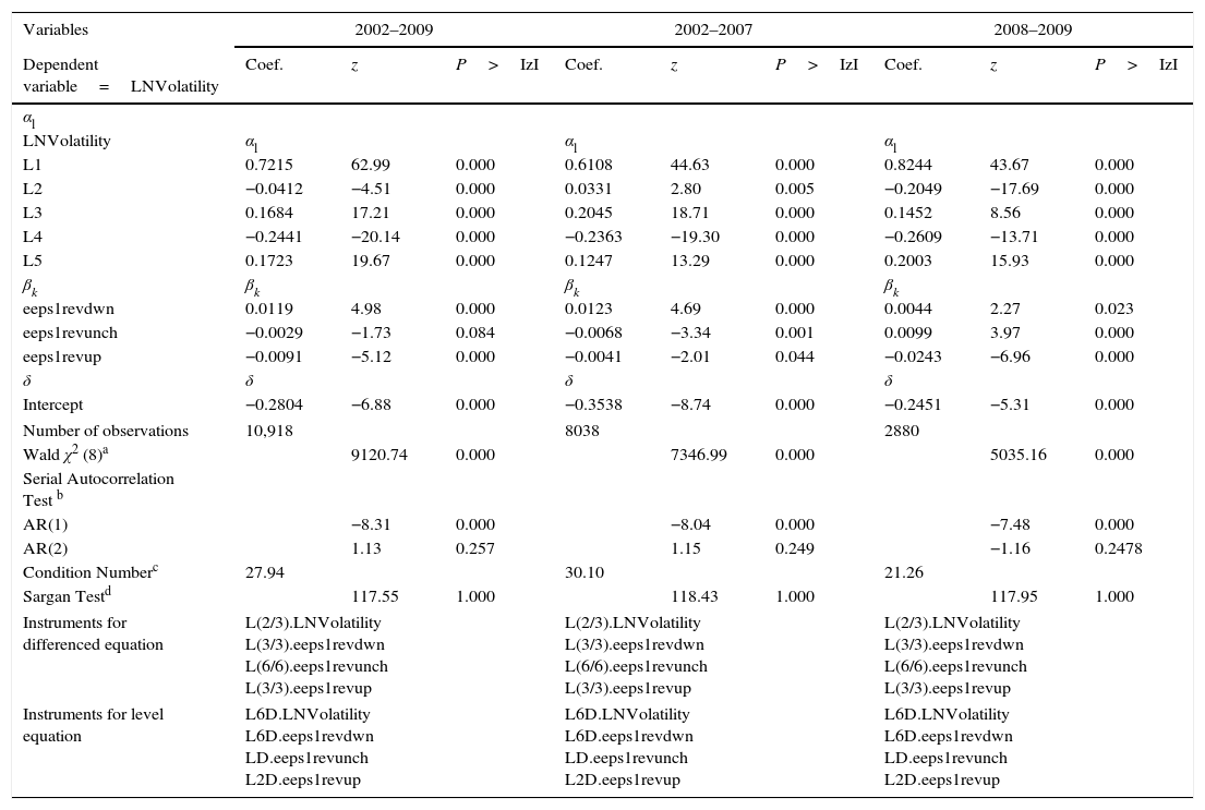
This table reports the result when volatility are regressed on various explanatory variables. LNVolatility is the monthly volatility and is estimated as the dependent variable, capturing market reactions to financial analysts’ consensus forecasts through a DPD model in differences and in two steps (Arellano and Bond, 1991). Monthly volatility is calculated using the GARCH (1,1) model (Bollerslev, 1986); LNVolatility L1, L2, L3, L4, and L5, are the monthly volatility lagged one, two, three, four, and five months; eeps1revup is the number of upward revisions of consensus earnings per share for the current year; eeps1revdwn is the number of downward revisions of consensus earnings per share for the current year; eeps1revunch is the number of monthly revisions that do not change consensus earnings estimates for the current year.
Model with recommendation revisions.
| Variables | 2002–2009 | 2002–2007 | 2008–2009 | ||||||
|---|---|---|---|---|---|---|---|---|---|
| Dependent variable=LNVolatility | Coef. | z | P>IzI | Coef. | z | P>IzI | Coef. | z | P>IzI |
| αl | |||||||||
| LNVolatility | αl | αl | αl | ||||||
| L1 | 0.7952 | 103.32 | 0.000 | 0.6611 | 47.98 | 0.000 | 0.8354 | 44.79 | 0.000 |
| L2 | −0.0442 | −6.39 | 0.000 | 0.0376 | 2.82 | 0.005 | −0.1860 | −6.91 | 0.000 |
| L3 | 0.1737 | 20.41 | 0.000 | 0.1985 | 18.5 | 0.000 | 0.2097 | 8.59 | 0.000 |
| L4 | −0.2204 | −24.07 | 0.000 | −0.2004 | −14.77 | 0.000 | −0.3072 | −17.76 | 0.000 |
| L5 | 0.1694 | 23.18 | 0.000 | 0.1300 | 10.52 | 0.000 | 0.1590 | 12.44 | 0.000 |
| βk | βk | βk | βk | ||||||
| redownward | −0.0063 | −3.43 | 0.001 | −0.0164 | −4.91 | 0.000 | 0.0274 | 4.18 | 0.000 |
| reunchanged | −0.0007 | −0.98 | 0.329 | −0.0024 | −2.61 | 0.009 | −0.0044 | −2.36 | 0.018 |
| reupward | 0.0111 | 5.50 | 0.000 | 0.0272 | 9.03 | 0.000 | −0.0190 | −3.37 | 0.001 |
| δ | δ | δ | δ | ||||||
| Intercept | −0.1532 | −9.26 | 0.000 | −0.2158 | −10.22 | 0.000 | −0.2089 | −5.04 | 0.000 |
| Number of observations | 10,918 | 8038 | 2880 | ||||||
| Wald χ2 (8)a | 23663.7 | 0.000 | 10087.46 | 0.000 | 6077.32 | 0.000 | |||
| Serial Autocorrelation Testb | |||||||||
| AR(1) | −8.37 | 0.000 | −7.83 | 0.000 | −7.16 | 0.000 | |||
| AR(2) | 1.64 | 0.102 | 1.31 | 0.191 | −0.09 | 0.9262 | |||
| Condition Numberc | 28.11 | 30.28 | 21.35 | ||||||
| Sargan Testd | 119.20 | 1.000 | 118.81 | 1.000 | 119.01 | 1.000 | |||
| Instruments for differenced equation | L(2/3).LNVolatility L(3/3).redownward L(6/6).reunchanged L(3/3).reupward | L(2/3).LNVolatility L(3/3).redownward L(6/6).reunchanged L(3/3).reupward | L(2/3).LNVolatility L(3/3).redownward L(6/6).reunchanged L(3/3).reupward | ||||||
| Instruments for level equation | L6D.LNVolatility L6D.redownward LD.reunchanged L2D.reupward | L6D.LNVolatility L6D.redownward LD.reunchanged L2D.reupward | L6D.LNVolatility L6D.redownward LD.reunchanged L2D.reupward | ||||||
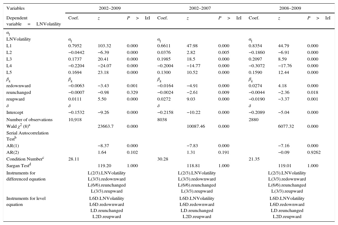
This table reports the result when volatility are regressed on various explanatory variables. LNVolatility is the monthly volatility and is estimated as the dependent variable, capturing market reactions to financial analysts’ consensus forecasts through a DPD model in differences and in two steps (Arellano and Bond, 1991). Monthly volatility is calculated using the GARCH (1,1) model (Bollerslev, 1986); LNVolatility L1, L2, L3, L4, and L5, are the monthly volatility lagged one, two, three, four, and five months; redownward: number of monthly downward revisions of consensus recommendation (an downward revision of a recommendation occurs when there is a change in the level of recommendation in the direction buy-hold-sell); reunchanged: number of monthly revisions in which the recommendation is unchanged; reupward: number of monthly upward revisions of consensus recommendation (an upward revision of a recommendation occurs when there is a change in the level of recommendation in the direction sell-hold-buy).
Models with significant variables.
| Variables | 2002–2009 | 2002–2007 | 2008–2009 | ||||||
|---|---|---|---|---|---|---|---|---|---|
| Dependent variable=LNVolatility | Coef. | z | P>IzI | Coef. | z | P>IzI | Coef. | z | P>IzI |
| αl | |||||||||
| LNVolatility | αl | αl | αl | ||||||
| L1 | 0.5822 | 38.05 | 0.000 | 0.5535 | 36.07 | 0.000 | 0.6285 | 14.18 | 0.000 |
| L2 | −0.0322 | −4.62 | 0.000 | 0.0315 | 1.59 | 0.112 | −0.1549 | −5.94 | 0.000 |
| L3 | 0.2052 | 29.72 | 0.000 | 0.2199 | 8.15 | 0.000 | 0.2228 | 15.53 | 0.000 |
| L4 | −0.2242 | −22.75 | 0.000 | −0.1920 | −13.55 | 0.000 | −0.2840 | −14.54 | 0.000 |
| L5 | 0.1679 | 15.15 | 0.000 | 0.1140 | 8.15 | 0.000 | 0.2336 | 12.11 | 0.000 |
| βk | βk | βk | βk | ||||||
| tprevdwn | 0.0365 | 23.26 | 0.000 | 0.0407 | 14.56 | 0.000 | 0.0407 | 11.01 | 0.000 |
| eeps2revdwn | −0.0085 | −7.44 | 0.000 | −0.0085 | −5.08 | 0.000 | −0.0172 | −8.5 | 0.000 |
| reupward | 0.0264 | 10.28 | 0.000 | 0.0291 | 8.7 | 0.000 | 0.0141 | 1.76 | 0.078 |
| δ | δ | δ | δ | ||||||
| Intercept | −0.482 | −22.3 | 0.000 | −0.4606 | −17.72 | 0.000 | −0.4574 | −7.5 | 0.000 |
| Number of observations | 10,918 | 8038 | 2880 | ||||||
| Wald χ2 (8)a | 15641.2 | 0.000 | 8337.27 | 0.000 | 4540.51 | 0.000 | |||
| Serial Autocorrelation Testb | |||||||||
| AR(1) | −8.22 | 0.000 | −7.94 | 0.000 | −6.6577 | 0.000 | |||
| AR(2) | 1.63 | 0.102 | 1.06 | 0.291 | −0.05971 | 0.9524 | |||
| Condition numberc | 27.09 | 29.24 | 21.09 | ||||||
| Sargan Testd | 117.24 | 1.000 | 118.27 | 1.000 | 118.415 | 1.0000 | |||
| Instruments for differenced equation | L(2/3).LNVolatility L(3/3).tprevdwn L(6/6).eeps2revdwn L(3/3).reupward | L(2/3).LNVolatility L(3/3).tprevdwn L(6/6).eeps2revdwn L(3/3).reupward | L(2/3).LNVolatility L(3/3).tprevdwn L(6/6).eeps2revdwn L(3/3).reupward | ||||||
| Instruments for level equation | L6D.LNVolatility L6D.tprevdwn LD.eeps2revdwn L2D.reupward | L6D.LNVolatility L6D.tprevdwn LD.eeps2revdwn L2D.reupward | L6D.LNVolatility L6D.tprevdwn LD.eeps2revdwn L2D.reupward | ||||||
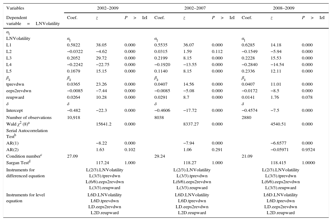
This table reports the result when volatility are regressed on various explanatory variables. LNVolatility is the monthly volatility and is estimated as the dependent variable, capturing market reactions to financial analysts’ consensus forecasts through a DPD model in differences and in two steps (Arellano and Bond, 1991). Monthly volatility is calculated using the GARCH (1,1) model (Bollerslev, 1986); LNVolatility L1, L2, L3, L4, and L5, are the monthly volatility lagged one, two, three, four, and five months; tprevdwn is the number of monthly downward revisions of consensus target price; eeps2revdwn is the number of downward revisions of consensus earnings per share for the end of the following year; reupward: number of monthly upward revisions of consensus recommendation (an upward revision of a recommendation occurs when there is a change in the level of recommendation in the direction sell-hold-buy).
The following are the supplementary data to this article:
The author gratefully acknowledges the research assistance of professors Teresa Corzo and Ricardo Gimeno. The author also thanks professor Margarita Prat for her valuable comments.

