


The relevance of systemic risk was highlighted by the economic and financial crisis starting in mid-2007. Supervisors and regulators recognized the need to improve the process of identification, management and mitigation of systemic risk. This paper introduces a Spanish Financial Market Stress Indicator (FMSI), similar to the “Composite Indicator of Systemic Stress” that Holló et al. (2012) proposed for the euro area as a whole. This indicator, which represents a real-time measure of systemic risk, tries to quantify stress in the Spanish financial system and describes the contribution of each financial market segment (bond market, equity market, money market, financial intermediaries, forex markets and derivatives) to the total stress in the system. The methodology takes into account time-varying correlations between market segments. The study analyses the ability of the FMSI to identify past periods of high financial stress and presents two econometric approaches with the aim of classifying observations into different stress regimes and of determining if financial stress has a negative impact on the real economy.
The global economic and financial crisis that many economies suffered after the collapse of Lehman Brothers in 2008 highlighted the importance of systemic risk. Following the crisis, authorities and financial supervisors realized that the identification of systemic risks deserved more attention. There was also a revision to the definition of systemic risk published by international institutions (IMF, FBS, BIS and IOSCO). One of the main lessons of this process was the recognition of the role that both banking and securities regulators had to play in this area. There have been many and various studies looking at some aspect of systemic risk in recent years. In general, current research is related to one or more relevant factors when considering systemic risk: size, interconnectedness, lack of substitutes and concentration, lack of transparency, leverage, market participant behaviour, information asymmetry and moral hazard.
There is a group of papers that, with the objective of measuring systemic risk, have developed Financial Stress Indexes (FSI) or fragility indexes. Some of these are coincident measures (like thermometers) that try to capture the level of financial stress in real time and others are forward-looking indicators. Other approaches have in common the definition of systemic risk as an extreme loss on a portfolio of assets related to financial intermediaries’ balance sheets. This definition of systemic risk focuses on the financial health of intermediaries, rather than on monetary and credit conditions. Finally, during the global financial and economic crisis, and especially in the context of the European sovereign debt crisis, many studies focused on the phenomenon of contagion.
This paper introduces a Spanish Financial Market Stress Indicator (FMSI), similar to the “Composite Indicator of Systemic Stress” that Holló et al. (2012) proposed for the euro area as a whole. This kind of indicator, which can be included in the group of Financial Stress Indicators (FSI), represents a coincident measure of systemic risk and tries to quantify and summarize the stress in the Spanish financial system in a single statistic. As well as summarizing the statistical design of the indicator, we provide a threefold evaluation of the FMSI and propose some applications in the context of the CNMV's supervisory duties.
The remainder of the paper is structured as follows: Section 2 summarizes the background and academic literature regarding systemic risk and explains the motivation for this paper. Section 3 provides the details of the statistical design of the Spanish FMSI, including the selection of markets and variables, the construction of the sub-indices and their aggregation into the composite indicator. Section 4 evaluates the indicator in terms of its ability to identify past episodes of stress in the Spanish financial system. This section also presents the results of two econometric approaches related to the theory of switching regimes and to the potential impact of financial stress on domestic output. Finally, Section 5 lays out the main conclusions.
2Theoretical background and related literatureFollowing the global financial crisis, which started by mid-2007, international authorities and governments realized that financial stability analysis and the process of identification of systemic risks should receive more attention. In their conclusions it was clear that both banking and securities regulators had to play a role in this area. In 2009, the International Monetary Fund (IMF), the Financial Stability Board (FSB) and the Bank of International Settlements (BIS) set out an approach to assessing the systemic importance of financial institutions, markets and instruments. These institutions described systemic risk as: “[…] the risk of disruption to financial services that is (i) caused by an impairment of all or parts of the financial system and (ii) has the potential to have serious negative consequences for the real economy2.”
In 2010 the Board of the International Organization of Securities Commissions (IOSCO) adopted two new principles (6 and 7) related to the process of monitoring, mitigating and managing systemic risk and to the process of reviewing the perimeter of regulation. Moreover, in 2011, IOSCO published a definition of systemic risk very close to that of IMF/FSB/BIS: “Systemic risk refers to the potential that an event, action, or series of events or actions will have a widespread adverse effect on the financial system and, in consequence, on the economy3”.
However, IOSCO elaborated on this definition, enumerating several factors which potentially can increase systemic risk. They mentioned the design, distribution or behaviour under stressed conditions of certain investment products, the activities or failure of a regulated entity, a market disruption or an impairment of a market's integrity. From IOSCO's perspective systemic risk can also take the form of a more gradual erosion of market trust caused by inadequate investor protection standards, lax enforcement, insufficient disclosure requirements, inadequate resolution regimes or other factors.
The academic research community has pursued a plentiful variety of approaches in the area of financial stability.4 In general, academic research has concentrated on one or more relevant factors to consider when assessing systemic risk: size, interconnectedness, lack of substitutes and concentration, lack of transparency, leverage, market participant behaviour, information asymmetry and moral hazard. A vast number of papers are based on banking industry data, as it was considered the main source of systemic risk.5 Since the beginning of the global financial crisis, many empirical studies have been performed on the basis of a more global approach.
There are several broad streams of studies that involve some kind of evaluation of systemic risk. There is a group of papers that, with the objective of measuring systemic risk, have developed Financial Stress Indexes (FSI) or fragility indexes. Some of these are coincident measures (like thermometers) that try to capture the level of financial stress on real time. Others are forward-looking indicators that, for example, calibrate the likelihood of simultaneous failure of a large number of financial intermediaries. The study of Illing and Liu (2006) can be considered as a seminal paper in this category. They develop a FSI for the Canadian financial system and propose several approaches to aggregate individual stress indicators into a composite stress index. Other relevant papers are Nelson and Perli (2007), Kritzman et al. (2010), Caldarelli et al. (2009), and Holló et al. (2012). Holló et al. (2012) perform a Composite Indicator of Systemic Stress (CISS) for the euro area, based on data of five segments of European financial markets (equity markets, bond markets, money markets, financial intermediaries and forex markets). They compute the Cumulative Distribution Function (CDF) of fifteen variables and take into account potential cross-correlations between market segments.
Other approaches have in common the definition of systemic risk as an extreme loss on a portfolio of assets related to financial intermediaries’ balance sheets. This definition of systemic risk focuses on the financial health of intermediaries, rather than on monetary and credit conditions. Examples of this methodology can be found in Segoviano and Goodhart (2009), Acharya et al. (2010), Adrian and Brunnermeier (2011), Huang et al. (2011), Gray and Jobst (2011), Brownlees and Engle (2012) and Hovakimian et al. (2012).
During the global financial and economic crisis, and especially in the context of the European sovereign debt crisis, many studies focused on the phenomenon of contagion. Relevant papers in this topic are Forbes and Rigobon (2001), Hyde et al. (2007), Diebold and Yilmaz (2009), Billio et al. (2010) and Caporin et al. (2013). Some studies show that correlations tend to increase during market crashes. As a consequence, the exposure to different countries’ equity markets offers less diversification in down markets than in up markets. This pattern has been shown to apply in other industries also6 (affecting the returns of global industries, individual stocks, hedge funds and international bond markets). The presence of sudden regime shifts, considered by some authors as a symptom of systemic risk, has also been tested by many studies. In general there is a perception that every economy shows two types of regimes: regimes of GDP growth and low volatility and regimes characterized by GDP contraction and high volatility (usually in the context of high uncertainty). Several papers show the existence of sudden regime shifts not only in the context of GDP but also in other economic or financial areas of interest like short-term interest rates, inflation or market turbulence.7
This paper introduces a Spanish Financial Market Stress Indicator (FMSI), similar to the “Composite Indicator of Systemic Stress” that Holló et al. (2012) proposed for the euro area as a whole.8 This kind of indicator, which can be included in the group of Financial Stress Indicators (FSI), represents a coincident measure of systemic risk and tries to quantify and summarize the stress in the Spanish financial system in a single statistic. Of course, this kind of approach may have some disadvantages due to the potential excessive simplification in the evaluation of systemic risk. However, it offers some useful characteristics. Firstly, it allows the real-time evaluation of financial stress in the whole financial system and the identification of past episodes of financial stress. Secondly, it can provide the basis information for an early warning signal model that assesses when the system may be nearing a high financial stress episode. It can also be used to test the impact of any policy measure regarding financial stability.
One of the major strengths of the Spanish FMSI is related to its ample coverage of the financial system. As we stated earlier, one of the main lessons drawn from the financial crisis was the importance of the financial sector as a whole and not only the banking sector as a potential source of generating and propagating systemic risk. Taking these considerations into account, and following the approach of Holló et al. (2012), we have computed information on six financial market segments that we consider crucial to evaluating any potential source of financial stress: the money market, equity market, bond market, financial intermediaries, derivatives market and forex market9 (see Fig. 1). Although this indicator represents a considerable improvement with respect to previous indicators in terms of the quantity and quality of data and of its coverage of the financial system, it is necessary to highlight two limitations. Firstly, financial intermediaries’ information is basically banking sector information and only some insurance companies’ data has been included. As part of its supervisory duties, the CNMV receives data on other relevant financial intermediaries such as mutual funds and investment services firms but not at the desired frequency (daily). Secondly, the indicator does not include information on financial infrastructure due to a lack of data.

Our Spanish FMSI comprises 18 market-based financial stress variables equally split into the six financial segments mentioned above. Stress in financial markets is characterized by the increase in uncertainty, the asymmetry of information and the rise in the risk aversion among investors (preference for safer and more liquid assets). Our 18 stress variables that, in general, represent changes in volatility, credit spreads, liquidity and loss of value in different instruments can be considered as good indicators of these characteristics of stress in financial markets.
Under the methodology of Holló et al. (2012), we compute the empirical CDF of each variable and construct a separate financial stress sub-index for each of the six financial segments considered. In order to aggregate these sub-indices into the global Spanish FMSI we also apply basic portfolio theory, which is one of the most important methodological innovations of our reference paper. This portfolio-theoretic aggregation takes into account the time-varying cross-correlations between our six sub-indices. As a consequence of this methodology, our Spanish FMSI puts relatively more weight on high stress financial situations, due to the fact that stress tends to be high in several market segments at the same time. At the end, we try to capture the situation when financial instability is spread across the whole financial system after systemic risk materializes.
This study also connects with the literature related to switching regimes that was presented earlier. We estimate an autoregressive Markov-switching model in order to identify the potential existence of different financial stress regimes according to the data provided by the FMSI. This kind of methodology allows us to evaluate in real time the possibility of being near a high financial stress episode and, if this is the case, the adoption of relevant policy measures to mitigate the risk.
Finally, and taking into account that the propagation of a systemic risk should have some economic impact (according to all definitions of systemic risk), we estimate a threshold vector autoregression (TVAR) to assess the interaction between our Spanish FMSI and some measures of economic activity. We try to identify one FMSI threshold at or above which financial stress is really high and may have a strong negative effect on the real economy. The relationship between financial system and real economy has also been explored by many studies.10
3Statistical design of the Spanish FMSI3.1Selection of markets and variablesIn order to measure systemic risk across the Spanish financial system, we consider the money market, bond market, equity market, financial intermediaries, foreign exchange market and derivatives market as good representations of different segments of the financial system. Each of these segments will be presented as a sub-index of the FMSI and will provide specific information for our composite indicator.
We include three variables in each of the market segments, so that the composite indicator comprises 18 individual stress indicators, with the aim of measuring systemic risk in real time. For that purpose, we use data which is available on a daily or weekly basis. We basically include asset return volatilities, risk spreads and liquidity indicators to capture the main symptoms of financial stress. Long-term variables have been computed in order to cover as many financial stress episodes and business cycles as possible. The three variables in each market segment should provide complementary information to the indicator, although we expect a high correlation between them during episodes of high financial stress (Holló et al., 2012).
In what follows, a brief description of each market, their compounded variables11 and the data source is presented and organized by the representative market segment.12
- •
Money market: this sub-index should reflect liquidity and counterparty risk in the inter-bank market (Heider et al., 2010 or Acharya and Skeie, 2011). In general, money market variables capture some features like flight-to-quality and flight-to-liquidity effects, as well as the price impacts of adverse selection problems in banking during stress periods.
- ∘
Realized volatility of the three-month Euribor rate: realized volatility calculated as the weekly average of absolute daily rate changes, transformed by its recursive sample CDF. Data start 30 Dec. 1998. Source: Thomson Datastream. The volatility can reflect features like flight-to-quality, flight-to-liquidity and/or increasing asymmetric information; therefore a positive relationship with systemic risk is highly expected.
- ∘
Interest rate spread between three-month Euribor and three-month Spanish Treasury Bills: weekly average of daily data, transformed by its recursive sample CDF. Data start 30 Dec. 1998 and 24 Mar. 1988 respectively. Source: Thomson Datastream. This variable represents a measure of liquidity and counterparty risk, and shows the convenience premium on short-term Treasury paper.
- ∘
Three-month Libor-OIS spread: weekly average of daily difference between three-month OIS and three-month Libor data, transformed by its recursive sample CDF. Data start 30 Dec. 1998 and 17 May. 1999 respectively. Source: Thomson Datastream. It is a measurement of liquidity and credit risk and also reflects the risk premium associated with lending to commercial banks. Therefore spread increases can be interpreted as a signal of high vulnerability in the financial system.
- ∘
- •
Bond market: Movements in this market are related to sovereign risk and concerns about solvency and liquidity conditions in the corporate bond market. They can also be a consequence of an increase in the uncertainty or the risk aversion of investors. In addition sudden variations of the variables included in this market will have considerable impact not only on financial institutions but also on households.
- ∘
Realized volatility of the Spanish ten-year benchmark government bond index: weekly average of absolute daily yield changes, transformed by its recursive sample CDF. Data start 4 Apr. 1991. Source: Thomson Datastream. Increases in the volatility can be a consequence of investor's concerns about Government default risk.
- ∘
Yield spread between the Spanish ten-year government bond and German ten-year government bond: weekly average of daily difference between Spanish and German ten-year bonds, transformed by its recursive sample CDF. Data start 4 Apr. 1991 and 1 Jan. 1980 respectively. Source: Thomson Datastream. This variable is a measure of sovereign risk premium as long as the German bond is considered the safest and most liquid sovereign bond of the euro area.
- ∘
Bid-ask spread of Spanish government bonds: weekly average of daily bid-ask spread, transformed by its recursive sample CDF. Data start 11 Aug. 1997. Source: Bloomberg. This variable reflects liquidity conditions in bond markets.
- ∘
- •
Equity markets: equity market variables capture shifts in volatility, liquidity and sudden asset price movements that are common in periods of financial stress.
- ∘
Volatility of Spanish non-financial corporation index: weekly average of absolute daily log returns of the non-financial sector stock market index, transformed by its recursive sample CDF. Data start 2 Mar. 1987. Source: Thomson Datastream. In general, asset price volatility indicators point to stress in the stocks markets.
- ∘
CMAX of Spanish non-financial corporation index: weekly average of daily maximum cumulated index losses of Spanish non-financial corporation index, over a moving two-year window, transformed by its recursive sample CDF. Data start 2 Mar. 1987. Source: Thomson Datastream. The CMAX13 measurement is used to determine periods of crisis in international equity markets (Patel and Sarkar (1998) and Coudert and Gex (2006)), but most recently is often used as an input in stress indicators (Illing and Liu, 2006). Significant falls in price assets are captured by high levels of this variable.
- ∘
Ibex 35 liquidity: weekly average of daily bid-ask spread, transformed by its recursive sample CDF. Data start 9 Jul. 2003.14 Source: Thomson Datastream. High financial stress levels are usually accompanied by drops in equity liquidity.
- ∘
- •
Financial intermediaries: Financial intermediaries play a major role in the correct functioning of the financial system. High increases in stress conditions for these institutions can be spread across the financial system and potentially have a strong negative impact on the real economy. The variables included in this market refer to volatility, credit risk and price movements.
- ∘
Realized volatility of the idiosyncratic equity return of the banking sector market index relative to Ibex 35 returns: idiosyncratic return calculated as the intercept from an OLS regression of daily log bank returns on the log market return over a moving two-year window; realized volatility calculated as the weekly average of absolute daily idiosyncratic returns, transformed by its recursive sample CDF. Data start 2 Mar. 1987. Source: Thomson Datastream. Increases in this indicator are interpreted as investors’ experiencing high uncertainty and/or concerns about banking sector default risk.
- ∘
Financial sector credit risk spread: weekly average of daily CDS of five important Spanish banks, transformed by its recursive sample CDF. Data start 2 Jul. 2007.15 Source: Thomson Datastream. High values in risk premium of these institutions imply a worsening in financing conditions that could be disseminated across the economy.
- ∘
CMAX of financial sector index combined with the inverse of its price-book ratio: weekly average of daily maximum cumulated index losses of Spanish financial sector index, over a moving two-year window and the inverse of the price-book ratio of these market, both transformed by their recursive sample CDF and then multiplied together. The final variable is obtained by taking the square root of this product. Data start 2 Mar. 1987 and 1 Jan. 1990 respectively. Source: Thomson Datastream. High values of this variable are a consequence of high values in CMAX and in price-book ratio, which means that the present market value of a corporation has fallen significantly below its book value.
- ∘
- •
Foreign Exchange market: this sub-index reflects large movements in foreign exchange markets. These movements are particularly relevant for those institutions heavily dependent on non-domestic liabilities and also for those with a high exposure to non-domestic assets.
- ∘
Realized volatility of the euro exchange rate vis-à-vis the US dollar: weekly average of absolute daily log foreign exchange returns, transformed by its recursive sample CDF. Data start 1 Jan. 1980. Source: Thomson Datastream.
- ∘
Realized volatility of the euro exchange rate vis-à-vis the Japanese Yen: weekly average of absolute daily log foreign exchange returns, transformed by its recursive sample CDF. Data start 1 Jan. 1980. Source: Thomson Datastream.
- ∘
Realized volatility of the euro exchange rate vis-à-vis the British Pound: weekly average of absolute daily log foreign exchange returns, transformed by its recursive sample CDF. Data start 1 Jan. 1980. Source: Thomson Datastream.
- ∘
- •
Derivatives market: Derivatives markets represent a special segment of the financial system in the sense that they are based upon another market, the underlying market. Their potential role in systemic risk was recognized by authorities during the last crisis, and has prompted some reforms, for example, in the OTC derivatives segment. The fluctuation of some relevant indicators of these markets can also be interpreted as signs of increasing uncertainty, risk aversion and financial stress.
- ∘
Realized volatility of IBEX-35 options: weekly average of daily implicit volatility of the IBEX 35 index, transformed by its recursive sample CDF. Data start 4 Jan. 1999. Source: Thomson Datastream.
- ∘
Realized volatility of IBEX-35 future open position: weekly average of daily volatility of the MEFF-IBEX 35 open interest index over a 60-day moving window, transformed by its recursive sample CDF. Data start 20 Apr. 1992. Source: Thomson Datastream.
- ∘
Realized volatility of commodities index: weekly average of daily oil price volatility, transformed by its recursive sample CDF. Data start 1 Jan. 1980. Source: Thomson Datastream.
- ∘
In order to obtain a unique sub-index for each of the representative markets, it is necessary to transform each raw variable into a standardized one and then aggregate these new variables. The academic literature suggests several methodologies for transforming the variables. For example, Morris (2010) proposes an empirical normalization which consists of subtracting the sample mean of the variable and dividing this difference by the sample standard deviation. Louzis and Vouldis (2012) follow a logistic transformation in order to standardize the raw variables. However, these approaches are based on the assumption of normally distributed variables, an assumption that is often violated by the nature of the financial market indicators. This fact implies some kind of robustness problems with the composite indicator. Requiring robustness in the time dimension is an important issue in order to create a real-time indicator, especially if it is going to be used as an early warning signal. For this reason we have used the transformation based in the empirical cumulative distribution function (CDF), such as in Holló et al. (2012).
Let us denote the data set of a particular variable xt as x=(x1,x2,…,xn) with n the total number of observations in the sample. The ordered sample is denoted (x1,x2,…,xn) where x1≤x2≤…≤xn and r is referred to as the ranking number assigned to a particular realization of xt. The values in the original data set are arranged such that xn represents the sample maximum and xn represents the sample minimum. The transformed variables zt are then computed from the original variables xt on the basis of the empirical CDF Fnxt as follows:
for t=1,2,…,n. The empirical CDF Fnx* measures the total number of observations xt not exceeding a particular value x* (which equals the corresponding ranking number x*) divided by the total number of observations in the sample (see Spanos, 1999). If a value x occurs more than once, the ranking number assigned to each of the observations is set to the average ranking. The empirical CDF is hence a function which is non-decreasing and piecewise constant with jumps being multiples of 1/n at the observed points. This results in transformed variables which are unit-free and measured on an ordinal scale with range (0,1].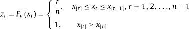
This transformation is applied recursively over expanding samples in order to feature the real-time character of the indicator. The pre-recursion period for each variable runs from its first historical value to 4 January 2002, and all subsequent observations are transformed recursively on the basis of ordered samples recalculated with one new observation added at a time:
for T=1,2,…,N with N indicating the end of the full data sample.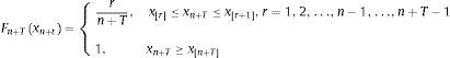
Once the transformation of the three stress factors (j=1,2,3) for each market (i=1,2,3,4,5,6) is computed, we end up with a data set of 18 homogenized stress factors. In order to obtain markets’ sub-indices, we perform the arithmetic average16 of the homogenized stress factors, which implies that each factor is equally weighted within the sub-index.
3.3Aggregation of sub-indices into the composite indicator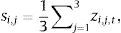
The next step is the aggregation of the six sub-indices into a simple indicator to measure the systemic stress. Following standard portfolio theory; we have taken into account cross-correlations between individual assets returns. The methodology was proposed by Holló et al. (2012) and also implemented by and Louzis and Vouldis (2012), Milwood (2012) and Cabrera et al. (2014), for the design of systemic risk indicators in Greece, Jamaica and Colombia, respectively. Proceeding under this theory, the composite indicator puts more emphasis on situations where stress is predominant in several markets at the same time. The idea underlying this approach is to capture systemic risk in the sense that high financial instability is disseminated across the financial system.
Each sub-index weight can be determined on the basis of the relative importance of this particular market for real economy activity.17 The weights we have applied here are the following: 15% for money market, 20% for the bond market and equity market, 30% for financial intermediaries, 5% for the foreign exchange market and 10% for derivatives. In order to incorporate the correlation between sub-indices, we compute a unit-free indicator, bounded by the half-open interval (0, 1], according to:
where w=(w1,w2,w3,w4,w5,w6) is defined as the vector of constant sub-index weights, st=(s1,t,s2,t,s3,t,s4,t,s5,t,s6,t) is the vector of sub-indices, and w∘st is the Hadamard-product.18Ct is the 6x6 matrix of time-varying cross-correlation coefficients ρij,t between sub-indices i and j, represented as:
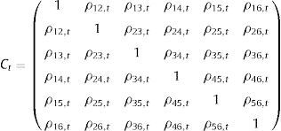
Time-varying cross-correlations ρij,t are performed recursively on the basis of exponentially weighted moving averages (EWMA) of respective covariances σij,t and volatilities σij,t as approximated by the following formulas:
where i=1,…,6, j=1,…,6, t=1,…T with s˜i,t=(si,t−0.5) represented the demeaned sub-indices obtained by subtracting the theoretical mean of each indicator. The decay factor or smoothing parameter λ is held constant through time at 0.93, while the covariances and volatilities are initialized for t=0 at their average values over the pre-recursion period 1 January 1999 to 4 January 2002 (see Fig. 2).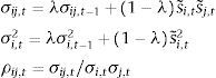

Cross-correlations between sub-indices.
Periods in which all correlations are close to one (see 2009) can be considered as extreme stress situations, as long as stress is spread across all financial markets. Nevertheless, high values in pair correlations only indicate stress in two markets in a certain period, which is not necessarily a signal of stress in the whole financial system.
3.4Backward extensionThis section presents the Spanish FMSI obtained after the computation of the stress variables and its aggregation according to the proposed methodology. Moreover, a backward extension of the indicator is provided in order to verify if our FMSI is able to capture important past events commonly known as high stress periods.
The Spanish Financial Market Stress Indicator shown in Fig. 3 provides a characterization of systemic risk in one single number and also the contribution of each market segment to this risk. Remember that the simple aggregation of these contributions does not correspond to the composite indicator, because our reference indicator takes into account cross market correlations. Both indicators tend to be similar when all our market segments are strongly correlated, usually in periods of high stress. This was the case in 2008 with the Lehman Brothers collapse but, in general, our composite indicator will be lower than the sum of the contributions. According to the results presented in Fig. 3, we can see the first high value of the indicator (0.41) in Sep. 2001,19 after the terrorist attacks in the US. Equity markets and financial intermediaries experienced high stress, which was not observed in other segments of financial markets. The second episode of high stress took place at the end of 2008, when the indicator reached its historical maximum (0.87). Finally, in the context of the European sovereign debt crisis, financial markets suffered several periods of high financial stress. The stress was particularly high in the Spanish financial system by mid-2011 and mid-2012, when the indicator reached a value of 0.69. In these episodes, financial intermediaries, bond markets and equity markets were the most stressed segments. In addition to the stress levels, Fig. 3 provides a first overview of correlation20 between markets.
.")
In the time period prior to 1999, there were several significant episodes of financial stress that deserve our attention because of its potential relevance in terms of systemic risk. We have performed a proxy for the FMSI which starts in Apr. 1987 with the historical data available in order to address this issue. The indicator presents some limitations due to the lack of data in some markets but in general it can be considered a good representation of financial stress in those years. As we can see from Fig. 4, where original and backward-extended FMSI are presented, at least two more periods of financial stress can be identified: one in Jan. 1991, when the FMSI reached a value of 0.52, and the other one in Oct. 1992, with a value of 0.66. These stress episodes are described in detail in Section 4.1.

Regarding correlation between sub-indices, we could say that during some periods of stress several correlations have been near one (which implies perfect correlation). In Fig. 5, the comparison between our reference FMSI and the indicator which assumes perfect correlation shows that in moments of high financial stress both indicators tend to be rather similar. On the contrary, in moments of low financial stress, which in our sample could be associated with the period between 1997 and 2004, both indicators tend to diverge because of the low correlation between market segments. In general, it can be concluded that under low stress periods, market segments performance reflects the idiosyncratic characteristics of each market.
3.5Robustness analysis
The construction of any indicator of systemic risk implies the adoption of some subjective decisions that can have significant consequences in terms of the properties of the indicator. We have performed some robustness checks in order to minimize some statistical problems. We are going to: (i) evaluate principal components analysis as aggregation method of transformed variables, (ii) modify market weights using those estimated by vector autoregression (VAR) models, (iii) change the value of the smoothing parameter and (iv) compare the results under recursive and non-recursive samples. In general, we conclude that our original Spanish FMSI is markedly robust and stable over time.
- •
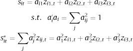
Principal component analysis (PCA): PCA is a statistical technique to simplify a data set that was developed by Pearson (1901) and Hotelling (1933). This technique transforms a large number of variables into a smaller number of uncorrelated (orthogonal) factors, called principal components. Each component is a linear combination of the original data and ordered in such a way that the first component accounts for the largest possible variance. We have computed a separate PCA for the variables of each sub-index and used the first component information to estimate the aggregate sub-index instead of the simple average of the three variables. As long as the composite indicator is ranged (0,1], the sub-indices have to be also ranged between 0 and 1. In order to estimate the new aggregate sub-indices capturing the maximum variance, the vector modulus should be 1. These sub-indices are computed as follows:
where sit* are the market sub-indices with i=1,2,3,4,5,6, aj represents the principal component coefficients of the first eigenvector with j=1,2,3 for each of the variables belonging to the six reference markets and zij,t the original variable data set.Fig. 6 displays the FMSI based on PCA aggregation methodology and the original FMSI. According to the estimates, both indicators are very similar and only small differences appear in 2002. See Coudert and Gex (2006) and Louzis and Vouldis (2012) for further information related to the application of PCA in risk indicators.
- •
Market weights: the selection of market weights can be done on the basis of VAR models and Impulse Response Functions (IRF) which are able to quantify the potential impact of financial shocks on real economy.21
The new financial market weights with this approach are as follows: 13% for the money market, 3% for the bond market, 18% for the equity market, 26% for financial intermediaries, 34% for the foreign exchange market and 7% for derivatives. In general, these weights are not very different from that used in the original FMSI except for the bond and forex markets. Fig. 7 presents a comparison between the original FMSI and the new-weighted FMSI. In general, both indicators are very similar. Only during the period 2000–2002 and in 2012 some differences are observed. During 2000–2002, the stress in forex markets at the beginning of the Monetary Union had a strong impact in the new-weighted FMSI because of the significant weight of this market in the index (34%). On the contrary, in 2012, the stress observed in bond markets had a smaller impact in the new FMSI. Due to the fact that both indicators are rather similar and that the original weights are perceived as more realistic,22 we still prefer the original version of the indicator.
- •
Changes in the smoothing parameter: exponential weighted moving averages are applied in order to decrease or eliminate the influence of random variations. Roberts (1959) defined λ as the smoothing parameter which determines the rate at which old data enter into the calculation of EWMA statistics. A large value of λ gives more weight to recent data and less weight to old data (and the contrary for small values of λ).
In Holló et al. (2012), the decay factor or smoothing parameter is held to be constant through time at a level of 0.93, which is an intermediate value. However, the authors computed the FMSI for other values of λ: 0.97 (high value) and 0.89 (low value). We have also estimated our Spanish FMSI for these three lambda values.
Fig. 8 illustrates small differences between the new indicators. It seems to be that the FMSI with a low smoothing parameter (λ=0.89) displays wide swings and spikes while the FMSI with a high parameter (λ=0.97) loses some power in the identification of some periods of stress (e.g. Sep. 2001). However, the differences are almost insignificant, so we can conclude that changes in the smoothing parameter do not imply any relevant alteration in the general behaviour of the indicator.
- •
Recursive versus non-recursive sample: we have computed the FMSI on a non-recursive basis. This implies the computation of CDF over the whole sample period (from Apr. 1987). The original FMSI, based on recursive empirical CDF starting in January 2002, and the non-recursive FMSI are very similar (see Fig. 9). There is only a small difference 2003.


The first exercise we can do to evaluate the Spanish FMSI is related to its ability to identify past stress episodes. In theory, the indicator should increase sizeably after a systemic risk event and reach unusually high levels. Hence, a formal evaluation of the indicator should take into account what a sizeable increase is and provide a definition of this unusually high level. Any kind of evaluation may experience type I errors, that is the failure to identify a high-stress event, and type II errors, which consists in a false identification of a high-stress event. Some evaluation approaches rely on “crisis defined by events” and others rely on “crisis defined by quantitative thresholds”. It is not possible to be sure that either of these approaches is the best option because both of them present problems. The “crisis defined by events” approach may miss some stress episodes that do not originate from a certain crisis event. The “crisis defined by quantitative thresholds” approach may incur type II errors (it is not necessarily true that when the FMSI is above a threshold, there is a systemic risk). Our evaluation, similar to Holló et al. (2012), is based on the analysis of the peaks of the Spanish FMSI during a very long time period. We test if these peaks can be associated with historical periods of stress or systemic events in order to verify potential type II errors (a false report of stress).
Fig. 10 illustrates the first significant hike of the historical Spanish FMSI in the summer of 1990, coinciding with the invasion of Kuwait by Iraq. This conflict prompted a sharp increase in oil prices and a decrease in risk appetite in global markets. There followed a period of intermediate financial stress, related to this geopolitical conflict. In 1992 there is a new historical maximum in the level of the indicator as a consequence of the European Exchange Rate Mechanism crisis. The huge tensions in the European exchange markets, which ended with the British Pound and the Italian Lira eventually leaving the system in September, were disseminated across global financial markets.

In the second quarter of 1994, an unexpected change in the monetary policy of the Federal Reserve prompted a significant increase in long-term interest rates across the world. In the Spanish securities markets, the huge growth in sovereign bond yields changed the perception of investors. Investors, especially non-residents, sold a big proportion of their equity holdings and increase their investment in bonds.
Between 1994 and 2001 there was a relatively long period of low stress in the financial system which was interrupted in September 2001, after the terrorist attacks in the US. Afterwards, the indicator stayed in a mid-financial stress level; probably as a consequence of the accounting scandals of 2002 and 2003 (Enron and Worldcom were the most significant episodes).
The maximum level of the Spanish FMSI was reached at the end of 2008, with the collapse of Lehman Brothers, although there was also a remarkable level of stress in financial markets in 2011–2012, during some episodes of turbulence in the context of the European sovereign debt crisis. The Spanish FMSI started to increase by mid-2007 when the first signs of the subprime crisis appeared and reached its historical maximum at the end of October (0.88), after the collapse of Lehman Brothers and the rescue of AIG. The high level of the indicator was maintained throughout the following weeks due to the uncertainty introduced by abandoning the plan to purchase toxic assets in the US. After that, the FMSI decreased sharply until it reached mid-levels of stress.
The last period of stress showed by the indicator must be understood in the context of the European sovereign debt crisis, as was said before. This crisis was characterized by the sharp increase of sovereign credit risk of those European countries perceived as more fragile in economic terms. During the crisis financial markets, and especially sovereign bond markets, equity markets and financial intermediaries suffered several episodes of extremely high stress. The first of these took place in May 2010 and was related to the potential Greek default. The second one started in the spring of 2011, when the Portuguese government asked for financial assistance. In the summer of 2011, extreme volatility in the markets prompted the ban on short selling by various European securities regulators. The CNMV also adopted this measure for financial sector firms. The level of financial stress continued to be very high during the following months, due to the perception of a second recession in Europe, until the events that in 2012 drove the indicator to its second historical maximum since 1987. In June 2012, the Spanish Government solicited European financial assistance for its banking sector and in July the CNMV adopted a second ban on short selling, which was applied to financial and non-financial firms. Although the level of systemic stress in Spain was really high in the summer of 2012, it was mainly concentrated in the bond market, the equity market and the financial intermediaries sector (banking). Cross-correlations between financial segments included in the FMSI were significantly lower than in the stress period related to the Lehman Brothers collapse, when cross-correlations were very high.
Based on this assessment, we can say that all the peaks of our Spanish FMSI can be related to one or various stress events, so the probability of type II errors is very limited (we will probably not make false systemic stress predictions). At the same time, although it is difficult to judge the probability of incurring type I errors (failure to identify high-stress events), it seems to be low. Periods of stress that we have not mentioned (for example, the Asian crisis in 1997 and the Russian default in 1998) are also identified by the Spanish FMSI, although the levels reached by the indicator are not as high as in other stress episodes.
4.2Regimes and thresholdsOnce the ability of the composite indicator of systemic stress to identify historical periods of financial stress is evaluated, we want to separate periods of high financial stress from periods of low and medium financial stress. The possibility of matching each value of the FMSI to one particular stress regime is very important for supervisors and policymakers. This classification can be considered as a tool to understand risks and evaluate potential causes of concern which, in some cases, may require policy actions.
There are several approaches that allow the classification of financial stress values of the indicator. A relatively simple approach is to classify financial stress as severe if the composite indicator exceeds the threshold of one standard deviation above its historical median or mean (Caldarelli et al., 2009). However, this approach presents several problems because it assumes that the indicator is normally distributed. According to the histogram for the FSMI presented in Fig. 11, we can conclude that the distribution of the indicator is multimodal and right-skewed. These properties suggest that the empirical density function of the FMSI is the result of the combination of several distributions representing different financial stress regimes.

In order to overcome the shortcomings of some methodologies, we apply an econometric approach similar to that suggested by Holló et al. (2012), which considers a regime classification based on an autoregressive Markov switching model. This approach allows us to model the dynamics of financial stress, based on the assumption that the time series properties of the FMSI are state-dependent. This means that financial stress tends to cluster displaying some intra-regime persistence, and that the transition between different states tends to occur stochastically.
For the purpose of determining this form of regime-dependence, we estimate several variants of a first-order autoregressive Markov switching model for the FMSI (Ft), with up to three states (st), where all coefficients are allowed to switch across states. The estimated coefficients by maximum likelihood are α(st) for the constant, β(st) for the lagged FMSI and σ(st)ut for the residual standard deviation, where the residuals ut are assumed to be white noise (standard, normal, independent and identically distributed (NID)).

We also assume that the stochastic process generating the states st follows an ergodic first-order Markov chain with transition probabilities p(st=i|st-1=j)=pi|j presented in the transition matrix P. This assumption implies that next period's regime only depends on the current regime but not on previous ones (Hamilton and Susmel (1994)).
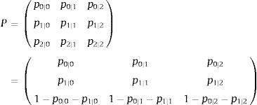
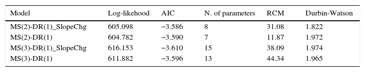
Table 1 presents some specifications tests for four autoregressive Markov switching models. We compute autoregressive process of order one (DR(1)) with two and three states or regimes. The intercept and the residual variance are allowed to switch in both models. The models labelled “SlopeChg” also allow for changes in the slope across regimes. According to the results, our preferred model specification is an autoregressive process of order one with three regimes in which all coefficients are allowed to switch (MS(3)-DR(1)_SlopeChg). This model presents the maximum log-likelihood value, the minimum AIC value and the null hypothesis of residuals being NID cannot be rejected. This model does not present the minimum value of the RCM statistic,23 although its value is low enough (38.09).
Testing different specifications of Markov-switching models for the Spanish FMSI.
| Model | Log-likehood | AIC | N. of parameters | RCM | Durbin-Watson |
|---|---|---|---|---|---|
| MS(2)-DR(1)_SlopeChg | 605.098 | −3.586 | 8 | 31.08 | 1.822 |
| MS(2)-DR(1) | 604.782 | −3.590 | 7 | 11.87 | 1.972 |
| MS(3)-DR(1)_SlopeChg | 616.153 | −3.610 | 15 | 38.09 | 1.974 |
| MS(3)-DR(1) | 611.882 | −3.596 | 13 | 44.34 | 1.965 |
MS(i)-DR(j) denotes an autoregressive Markov-switching model for the Spanish FMSI of order j with i states. The intercept and the residual standard deviation are allowed to change across regimes. The “_SlopeChg” models also allow for changes in the slope across regimes. AIC is the Akaike information criterion. The RCM is the regime classification method measure of Baele (2005). Durbin-Watson statistic tests the null hypothesis that the residuals are uncorrelated.
Estimations based on monthly data from Apr. 1987 to Jan. 2015.
Fig. 12 displays fitted values (top panel) and residuals (bottom panel) of our preferred model, which includes three states and varying coefficients across states (MS(3)-DR(1)_SlopeChg). Fig. 13 presents the estimated smoothed regime probabilities. Notice that regime 0 corresponds to low stress periods, whereas regime 1 represents intermediate stress periods and regime 2 depicts high stress periods. It is important to note that the smoothed probabilities of regime 2 (high stress periods) fit the major financial stress periods described in Section 4.1.
-DR(1) model. MS(3)-DR(1) denotes an autoregressive Markov-switching model for the Spanish FMSI of order 1 with 3 states. The intercept, the slope and the residual standard deviation are allowed to change across regimes. Estimations based on monthly data from Apr. 1987 to Jan. 2015.")
Fitted values and residuals for the MS(3)-DR(1) model. MS(3)-DR(1) denotes an autoregressive Markov-switching model for the Spanish FMSI of order 1 with 3 states. The intercept, the slope and the residual standard deviation are allowed to change across regimes. Estimations based on monthly data from Apr. 1987 to Jan. 2015.
-DR(1) model. MS(3)-DR(1) denotes an autoregressive Markov-switching model for the Spanish FMSI of order 1 with 3 states. The intercept, the slope and the residual standard deviation are allowed to change across regimes. Estimations based on monthly data from Apr. 1987 to Jan. 2015.")
Smoothed regime probabilities for the MS(3)-DR(1) model. MS(3)-DR(1) denotes an autoregressive Markov-switching model for the Spanish FMSI of order 1 with 3 states. The intercept, the slope and the residual standard deviation are allowed to change across regimes. Estimations based on monthly data from Apr. 1987 to Jan. 2015.
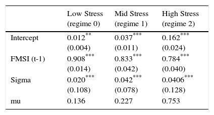
The estimated parameters of the autoregressive Markov-switching model of order one and three regimes where the coefficients are allowed to change across regimes are shown in Table 2. All estimated coefficients are highly significant statistically and differ substantially between the three regimes. The resulting unconditional mean level of the low stress regime amounts to 0.14 whereas the unconditional mean levels of the mid-stress and high-stress regimes are about 0.23 and 0.75, respectively. Even though the difference between the unconditional mean level in low and intermediate regimes is not significant, the volatility captured by these regimes differs substantially. The intermediate stress regime that our model estimates can be considered as an early warning signal because is characterized by relatively low values of the stress indicator but increasing volatility in the markets. As Fig. 14 illustrates, periods of high financial stress have always been preceded by periods of intermediate stress.
Parameter estimates of the MS(3)-DR(1) model.
| Low Stress (regime 0) | Mid Stress (regime 1) | High Stress (regime 2) | |
|---|---|---|---|
| Intercept | 0.012** (0.004) | 0.037*** (0.011) | 0.162*** (0.024) |
| FMSI (t-1) | 0.908*** (0.014) | 0.833*** (0.042) | 0.784*** (0.040) |
| Sigma | 0.020*** (0.108) | 0.042*** (0.078) | 0.0406*** (0.128) |
| mu | 0.136 | 0.227 | 0.753 |
MS(3)-DR(1) denotes an autoregressive Markov-switching model for the Spanish FMSI of order 1 with 3 states. The intercept, the slope and the residual standard deviation are allowed to change across regimes. Standard errors are reported in parentheses. “mu” stands for the unconditional mean in each regime. Estimations based on monthly data from Apr. 1987 to Jan. 2015.
-DR(1) model. MS(3)-DR(1) denotes an autoregressive Markov-switching model for the Spanish FMSI of order 1 with 3 states. The intercept, the slope and the residual standard deviation are allowed to change across regimes. Grey and red shaded areas correspond to periods of medium and high financial stress, respectively. Horizontal lines (“mu”) stand for the unconditional mean in each regime. Estimations based on monthly data from Apr. 1987 to Jan. 2015. Percentage of observations in each regime: 11.4% (high stress), 46% (intermediate stress) and 42.6% (low stress).")
Spanish FMSI and regimes of stress from MS(3)-DR(1) model. MS(3)-DR(1) denotes an autoregressive Markov-switching model for the Spanish FMSI of order 1 with 3 states. The intercept, the slope and the residual standard deviation are allowed to change across regimes. Grey and red shaded areas correspond to periods of medium and high financial stress, respectively. Horizontal lines (“mu”) stand for the unconditional mean in each regime. Estimations based on monthly data from Apr. 1987 to Jan. 2015. Percentage of observations in each regime: 11.4% (high stress), 46% (intermediate stress) and 42.6% (low stress).
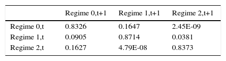
Both transition matrix parameters (Table 3) and representations of the three periods of financial stress depicted in Fig. 14 help to establish an economic interpretation. Regarding transition probabilities, we can see that when the FMSI reaches one stress regime, the most likely thing to happen is that it will stay in that regime. In this sense, the model illustrates a high degree of persistence. The more interesting results of this matrix, which represent a big difference from other studies, are the transition probabilities when the indicator is in a high stress regime. When financial stress is increasing, our model forecasts a regular transition process in which the FMSI moves from regime 0 (low stress) to regime 1 (mid stress) and from regime 1 to regime 2 (high stress). However, the inverse process is not observed when financial stress decreases. In these cases, it may be that after some public event, action or policy measure, the systemic risk level perceived by investors decreases fast prompting a sudden drop in the indicator to regime 0, skipping regime 1 (see Fig. 14).
Transition matrix of the MS(3)-DR(1) model.
| Regime 0,t+1 | Regime 1,t+1 | Regime 2,t+1 | |
|---|---|---|---|
| Regime 0,t | 0.8326 | 0.1647 | 2.45E-09 |
| Regime 1,t | 0.0905 | 0.8714 | 0.0381 |
| Regime 2,t | 0.1627 | 4.79E-08 | 0.8373 |
MS(3)-DR(1) denotes an autoregressive Markov-switching model for the Spanish FMSI of order 1 with 3 states. The intercept, the slope and the residual standard deviation are allowed to change across regimes. Estimations based on monthly data from Apr. 1987 to Jan. 2015.
In other words, this particular model applied to Spanish data suggests that periods of high stress in the financial system (red shaded area in Fig. 14) are preceded by periods of intermediate stress (grey shaded areas), whereas periods of high stress tend to finish very quickly (probably after a policy action) and are followed immediately by periods of low stress.
4.3Evaluation of potential real effectsBased on the “vertical perception” of systemic risk, financial stress should be a cause of concern for supervisors not only because of the impairment of the financial system itself but also because of the potential negative consequences for the real economy. This section analyses the relationship between financial stress and real economy. In this sense, it addresses the second part of the definition of systemic risk: “[…] the risk of disruption to financial services that is (i) caused by an impairment of all or parts of the financial system and (ii) has the potential to have serious negative consequences for the real economy.”
We apply a threshold regression model in order to determine the length and strength of financial shocks. In contrast to Markov-switching models,24 threshold regression models belong to a class of switching-regime models that assumes that state transitions are triggered any time an observable variable crosses a certain threshold level which needs to be estimated from the data. Following Tsay (1998), potential threshold effects within a bivariate threshold VAR model (TVAR) are determined, where the backward extended FMSI and annual growth in industrial production are given as endogenous variables. Fig. 15, which plots the FMSI and annual growth of industrial production, reveals that lower growth rates of industrial production can be associated with higher values of the FMSI.
.")
The basic threshold VAR regression setup is as follows:
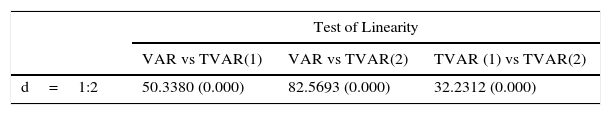
where xt=Ft,yt is the two dimensional vector of endogenous variables (the FMSI Ft and annual industrial production growth yt), cs,ϕjs the vector of intercepts and the two matrices of the slope coefficients for states s=H,M,L (with H,M and L standing for high-stress, mid-stress and low-stress regimes, respectively) and lags j=1,2. The threshold variable is denoted by zt−d where d∈1,…,d0 and d0=1 the maximum threshold lag or “delay” foreseen, tested following the AIC and BIC criteria as shown in Table 4. The threshold parameter is labelled τi with i=1,2 and the vector ets contains the state-dependent regression errors with variance-covariance matrices ∑ s=H,M,L .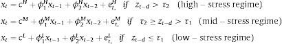
Testing the VAR versus TVAR and the threshold delay.
| Test of Linearity | |||
|---|---|---|---|
| VAR vs TVAR(1) | VAR vs TVAR(2) | TVAR (1) vs TVAR(2) | |
| d=1:2 | 50.3380 (0.000) | 82.5693 (0.000) | 32.2312 (0.000) |
| Testing threshold delay (d) and threshold values | ||||
|---|---|---|---|---|
| τ1 | τ2 | AIC | BIC | |
| d=1 | 0.2659 | 0.4903 | −5261.4 | −5139.7 |
| d=2 | 0.2022 | 0.2552 | −5229.7 | −5107.6 |
Test of linearity tests linear VAR (bivariate VAR with two lags) against TVAR(1) or TVAR(2). TVAR(1) denotes the bivariate threshold-VAR model with 2 lags, one threshold (two regimes) and the Spanish FMSI and annual growth in industrial production as endogenous variables. TVAR(2) denotes the bivariate threshold-VAR model with 2 lags, two thresholds (three regimes) and the Spanish FMSI and annual growth in industrial production as endogenous variables. TVAR(1) against TVAR(2) is also tested. The p-value is reported in parentheses. d denotes the threshold delay and τ the threshold value. AIC is the Akaike information criterion and BIC is the Bayesian information criterion. Monthly data from Apr. 1987 to Jan. 2015.
The previous model specification is based on the results of several tests, partially shown in Table 4. We test for the existence of threshold effects, which means testing a TVAR against a VAR model. According to the tests of linearity25 presented in Table 4, we reject the absence of linearity, so TVAR models are considered a better option. Moreover, tests on TVAR(1), which is a TVAR with 1 threshold or 2 regimes, against a TVAR(2), which is a TVAR with 2 threshold or 3 regimes, points to the existence of two relevant thresholds. We also test the threshold delay (d=1 or d=2). Information criteria (AIC and BIC) establish d=1 as the best option and the number of lags=2. Finally, we computed our preferred model that corresponds to a bivariate TVAR(2) with two lags, two thresholds (three regimes) and one threshold delay. The Spanish FMSI and the annual growth in industrial production are considered endogenous variables. Under this specification the estimated threshold values of the FMSI are 0.2659 and 0.4903.
Fig. 16 depicts the Spanish FMSI along with the estimations of the two threshold levels for the FMSI. According to the results, FMSI values below 0.2659 are considered low stress periods; FMSI values between 0.2659 and 0.4903 are considered mid-stress or intermediate stress periods and finally FMSI values above 0.4903 point to high-stress in financial markets. This econometric approach identifies three periods of high financial stress in the financial system: the European Exchange Rate Mechanism crisis in 1992, the financial crisis starting in mid-2007, and the European sovereign debt crisis. Other episodes of stress related to the Iraqi invasion of Kuwait in 1990, the change of US monetary policy in 1994 and the 9/11 terrorist attacks in 2001 can be considered periods of intermediate financial stress.

Stress regimes based on a bivariate threshold-VAR model with two lags, two thresholds (three regimes) and the Spanish FMSI and annual growth in industrial production as endogenous variables. High-stress regime occurs when the FMSI (once lagged) stands at or above 0.4903. Mid-stress regime occurs when the FMSI (once lagged) is between 0.2659 and 0.4903. Low-stress regime occurs when the FMSI (once lagged) is below 0.2659 Monthly data from Apr. 1987 to Jan. 2015.
Now, we address the issue of the expected negative impact of FMSI shocks in industrial production. A visual review of both variables (see scatter plot in appendix) suggest that for low FMSI values there is no relationship between these variables. However, for high FMSI values there seems to be a clear negative relationship between FMSI and industrial production. In a more technical way, we compute impulse response functions (IFR) from the estimated TVAR-coefficients for each of the three regimes of stress. Fig. 17 displays the results obtained from the triangular Choleski-factorisation or decomposition of the variance-covariance matrix of residuals. The dotted lines around the IRFs represent 95% confidence intervals.
 of industrial production growth to shocks in the FMSI from TVAR model.")
The estimation allows us to distinguish between real economic contemporaneous impact of financial stress across the three regimes which, according to Fig. 17, are very different. During low stress regimes, shocks in the FMSI do not exert any statically and economically significant reaction in output. On the contrary, intermediate and high stress regimes exert a negative reaction in industrial production. The maximum impact in mid-stress regime is reached 3 months after the FMSI shock with a decrease of annual output growth of 0.45%. It takes about six months to recover positive rates. In the case of high-stress regimes, the impact is much higher. This impact reaches the maximum level after 5 months, with a decrease of 1.5% in output growth in response to an initial shock in the FMSI. It takes about 8 months for the marginal effects to taper off.
TVAR denotes the bivariate threshold-VAR model with 2 lags, two thresholds (three regimes) and the Spanish FMSI and annual growth in industrial production as endogenous variables. High-stress regime occurs when the FMSI (once lagged) stands at or above 0.4903 (red line). Mid-stress regime occurs when the FMSI (once lagged) is between 0.2659 and 0.4903 (yellow line). Low-stress regime occurs when the FMSI (once lagged) is below 0.2659 (green line). Orthogonalised impulse response coefficients are computed. 95% confidence interval for the bootstrapped errors bands are reported (dotted lines). Monthly data from Apr. 1987 to Jan. 2015.
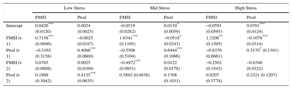
TVAR estimated coefficients are provided in Table 5 for the three stress regimes included in the model. It is important to notice the differences between the results of FMSI and industrial production equations. FMSI equation coefficients suggest a positive relationship between FMSI and its lagged values across the three stress regimes and no relationship between FMSI and output. Industrial production equation coefficients also suggest a positive relationship between output and its lagged values across all stress regimes. Additionally in the case of high and intermediate stress, the results points to a negative relationship between output and the first lag of FMSI, that is significant statistically. These coefficients are based on the negative response of output to shocks in the FMIS presented in Fig. 17. Causality Granger26 tests find out that shocks in the FMSI drive movements in industrial production, but not the opposite, reinforcing the results of the TVAR.
Parameter estimates of TVAR (two thresholds, three regimes).
| Low Stress | Mid Stress | High Stress | ||||
|---|---|---|---|---|---|---|
| FMSI | Prod | FMSI | Prod | FMSI | Prod | |
| Intercept | 0.0426*** (0.0120) | 0.0024 (0.0025) | −0.0519 (0.0282) | 0.0139* (0.0059) | −0.0591 (0.0595) | 0.0701*** (0.0124) |
| FMSI (t-1) | 0.7158*** (0.0896) | −0.0025 (0.0187) | 1.6341*** (0.1165) | −0.0518* (0.0243) | 1.3208** (0.1505) | −0.1078*** (0.0314) |
| Prod (t-1) | −0.3165 (0.3158) | 0.4086*** (0.0660) | −0.5508 (0.5104) | 0.6444*** (0.1066) | −0.8370 (0.6661) | 0.3170* (0.1391) |
| FMSI (t-2) | 0.0785 (0.0808) | 0.0025 (0.0169) | −0.4972*** (0.0851) | 0.0122 (0.0178) | −0.2502 (0.1542) | −0.0340 (0.0322) |
| Prod (t-2) | 0.1988 (0.3042) | 0.4135*** (0.0635) | 0.5892 (0.4938) | 0.1708 (0.1031) | 0.9207 (0.5778) | 0.2321 (0.1207) |
TVAR denotes the bivariate threshold-VAR model with 2 lags, two thresholds (three regimes) and the Spanish FMSI and annual growth in industrial production as endogenous variables. High-stress regime occurs when the FMSI (once lagged) stands at or above 0.4902993. Mid-stress regime occurs when the FMSI (once lagged) is between 0.2659278 and 0.4902993. Low-stress regime occurs when the FMSI (once lagged) is below 0.2659278. Standard errors are reported in parentheses. Percentage of observations in each regime: 63.9% (low-stress), 23.5% (mid-stress) and 12.7% (high-stress). Monthly data from Apr. 1987 to Jan. 2015.
The interaction between the FMSI and other macro variables provides similar results. Fig. A.2 shows the impulse response function computed from a model where the FMSI and annual change in exports are considered as endogenous variables. According to the results, in the case of high-stress regimes, the impact on exports of a shock in the FMSI reaches a maximum after five months, with a decrease of 2.5%. It takes ten months to recover positive rates.
We must bear in mind the pros and cons of these kind of methodologies. On one hand, our sample data is long enough to have a great variability, with many observations belonging to periods of high, intermediate and low financial stress. This characteristic makes us more confident in the results of the regression, in contrast with other studies that use sample data with only one period of high stress in financial markets. On the other hand, the bivariate model estimation as presented here does not include other explanatory variables that can potentially be relevant. We may have a mis-specification problem.
5ConclusionsThe latest global economic and financial crisis, which started in mid-2007, highlighted the relevance of systemic risk analysis and prompted many empirical studies in this area. International bodies redefined the concept of systemic risk and IOSCO established two new principles regarding systemic risk and the perimeter of regulation. The multiple analysis, which covers a high spectrum of possibilities, comprises a group of tools that tries to identify and quantify systemic risk and can be very useful for financial supervisors and regulators.
This paper presents a composite indicator of systemic stress in the Spanish financial system, similar to the indicator introduced by Holló et al. (2012) for the euro area. In our context, systemic risk is related to financial market stress, which is usually characterized by the increase in investors’ uncertainty, the asymmetry of information and the rise in risk aversion. Our Spanish Financial Markets Stress Indicator is based on 18 variables belonging to six segments of financial markets, which are considered good representations of stress in financial markets. These variables are mainly computed as volatilities, interest rate spreads, liquidity indicators and price movements. The segments of financial markets correspond to the money, bond and equity markets, financial intermediaries, foreign exchange markets and derivatives.
The methodology used to compute the indicator includes the transformation of raw variables through the empirical CDF performed recursively and the aggregation of series based on portfolio theory. This implies that the indicator puts more weight on situations where correlation between sub-markets is high, which is usually the case in periods of high financial stress. This approach provides a unique value of the indicator that quantifies the level of financial stress and illustrates the contribution to financial stress of these market segments. The FMSI, which can be performed in real time, also proved its robustness after several checks.
The evaluation of the FMSI addresses firstly its ability to detect past periods of financial stress. Taking into account data from our backward extended FMSI, which starts in 1987, we conclude that all observed peaks in the indicator correspond to very well-known periods of financial stress. Probabilities of Type I and Type II errors seem to be limited. The evaluation of our indicator is completed with two econometric estimations. The first econometric approach tries to separate FMSI observations into several groups of financial stress. We perform an autoregressive Markov-switching model which provides the probabilities of being in different stress regimes. Our preferred model includes three regimes of financial stress, with 12% of observations assigned to high-stress episodes. Under this methodology, high-stress episodes are always preceded by periods of intermediate stress, whereas after a high stress episode a sudden decrease of the FMSI is observed. The second econometric approach addresses the “vertical” perception of systemic risk and tries to estimate the impact of financial stress on the real economy. We compute a bivariate Threshold VAR (TVAR) model with three regimes, with FMSI and annual growth in industrial production being the endogenous variables. The estimated threshold values are 0.2659 and 0.4903. FMSI values below 0.2659 correspond to low-stress periods, FMSI values between 0.2659 and 0.4903 to intermediate-stress periods and FMSI values over 0.4903 can be considered high-stress. Impulse response functions computed for the different regimes show that in high stress periods, shocks in the FMSI have a strong negative impact on industrial production. This impact reaches the maximum level after 5 months, with a decrease of 1.5% in output growth in response to an initial shock in the FMSI. It takes about 8 months for the marginal effects to taper off.
In conclusion, we provide a robust measure of stress in Spanish financial markets that can be used to evaluate and quantify the level of systemic risk on real time. The FMSI, that has proved its ability to identify past periods of high financial stress, can be used by financial supervisors and regulators that are making bigger efforts in the process of identification, management and mitigation of systemic risks. The evaluation presented in this study provides some threshold values for the indicator which can be considered as an early warning signal and, potentially, prompt the adoption of proper policy measures.
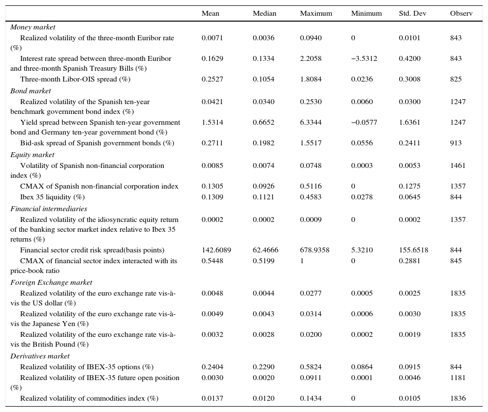
See Table A.1 and Figs. A.1 and A.2.
Summary of statistics.
| Mean | Median | Maximum | Minimum | Std. Dev | Observ | |
|---|---|---|---|---|---|---|
| Money market | ||||||
| Realized volatility of the three-month Euribor rate (%) | 0.0071 | 0.0036 | 0.0940 | 0 | 0.0101 | 843 |
| Interest rate spread between three-month Euribor and three-month Spanish Treasury Bills (%) | 0.1629 | 0.1334 | 2.2058 | −3.5312 | 0.4200 | 843 |
| Three-month Libor-OIS spread (%) | 0.2527 | 0.1054 | 1.8084 | 0.0236 | 0.3008 | 825 |
| Bond market | ||||||
| Realized volatility of the Spanish ten-year benchmark government bond index (%) | 0.0421 | 0.0340 | 0.2530 | 0.0060 | 0.0300 | 1247 |
| Yield spread between Spanish ten-year government bond and Germany ten-year government bond (%) | 1.5314 | 0.6652 | 6.3344 | −0.0577 | 1.6361 | 1247 |
| Bid-ask spread of Spanish government bonds (%) | 0.2711 | 0.1982 | 1.5517 | 0.0556 | 0.2411 | 913 |
| Equity market | ||||||
| Volatility of Spanish non-financial corporation index (%) | 0.0085 | 0.0074 | 0.0748 | 0.0003 | 0.0053 | 1461 |
| CMAX of Spanish non-financial corporation index | 0.1305 | 0.0926 | 0.5116 | 0 | 0.1275 | 1357 |
| Ibex 35 liquidity (%) | 0.1309 | 0.1121 | 0.4583 | 0.0278 | 0.0645 | 844 |
| Financial intermediaries | ||||||
| Realized volatility of the idiosyncratic equity return of the banking sector market index relative to Ibex 35 returns (%) | 0.0002 | 0.0002 | 0.0009 | 0 | 0.0002 | 1357 |
| Financial sector credit risk spread(basis points) | 142.6089 | 62.4666 | 678.9358 | 5.3210 | 155.6518 | 844 |
| CMAX of financial sector index interacted with its price-book ratio | 0.5448 | 0.5199 | 1 | 0 | 0.2881 | 845 |
| Foreign Exchange market | ||||||
| Realized volatility of the euro exchange rate vis-à-vis the US dollar (%) | 0.0048 | 0.0044 | 0.0277 | 0.0005 | 0.0025 | 1835 |
| Realized volatility of the euro exchange rate vis-à-vis the Japanese Yen (%) | 0.0049 | 0.0043 | 0.0314 | 0.0006 | 0.0030 | 1835 |
| Realized volatility of the euro exchange rate vis-à-vis the British Pound (%) | 0.0032 | 0.0028 | 0.0200 | 0.0002 | 0.0019 | 1835 |
| Derivatives market | ||||||
| Realized volatility of IBEX-35 options (%) | 0.2404 | 0.2290 | 0.5824 | 0.0864 | 0.0915 | 844 |
| Realized volatility of IBEX-35 future open position (%) | 0.0030 | 0.0020 | 0.0911 | 0.0001 | 0.0046 | 1181 |
| Realized volatility of commodities index (%) | 0.0137 | 0.0120 | 0.1434 | 0 | 0.0105 | 1836 |
 against industrial production (annual change).")
 of exports growth to shocks in the FMSI from TVAR model. TVAR denotes the bivariate threshold-VAR model with 2 lags, two thresholds (three regimes) and the Spanish FMSI and annual growth in exports as endogenous variables. High-stress regime occurs when the FMSI (once lagged) stands at or above 0.4903 (red line). Mid-stress regime occurs when the FMSI (once lagged) is between 0.2659 and 0.4903 (yellow line). Low-stress regime occurs when the FMSI (once lagged) is below 0.2659 (green line). Orthogonalised impulse response coefficients are computed. 95% confidence interval for the bootstrapped errors bands are reported (dotted lines). Monthly data from Apr. 1987 to Jan. 2015. (For interpretation of the references to color in this figure legend, the reader is referred to the web version of this article.)")
Impulse response functions (IRF) of exports growth to shocks in the FMSI from TVAR model. TVAR denotes the bivariate threshold-VAR model with 2 lags, two thresholds (three regimes) and the Spanish FMSI and annual growth in exports as endogenous variables. High-stress regime occurs when the FMSI (once lagged) stands at or above 0.4903 (red line). Mid-stress regime occurs when the FMSI (once lagged) is between 0.2659 and 0.4903 (yellow line). Low-stress regime occurs when the FMSI (once lagged) is below 0.2659 (green line). Orthogonalised impulse response coefficients are computed. 95% confidence interval for the bootstrapped errors bands are reported (dotted lines). Monthly data from Apr. 1987 to Jan. 2015. (For interpretation of the references to color in this figure legend, the reader is referred to the web version of this article.)
Mª Isabel Cambón and Leticia Estévez are both members of the Research, Statistics and Publications Department, CNMV (Spanish Securities Markets Supervisor).
See IMF-BIS-FSB (2009).
See IOSCO (2011).
See, for example, Rodríguez-Moreno and Peña (2013).
The Bank of Spain publishes a simpler version of this indicator in its Financial Stability Report (FSR). See box 1.1 in the May-13 FSR for details.
This market also includes information on oil prices.
In order to be consistent the same number of variables has been included in each market. Since the sub-indices are computed as simple averages, under the assumption of normally distributed variables, the inclusion of one additional variable in one particular market would reduce the variance of the average of the sub-index.
Summary statistics of the raw variables are provided in the annex.
CMAXt=1−xt/max[x∈(xt−j|j=0,1,…T)], where T=104 for weekly data.
From 1 Jan. 1999 to 9 Jul. 2003 Ibex 35 liquidity has been computed from Ibex 35's constituents; weekly average of daily bid-ask spreads. Time varying weights have been used.
From 1 Jan. 1991 to 1 Jul. 2007 financial sector credit risk spread has been estimated from the yield spread between European A-rated financial corporations and the ten-year Spanish government bond.
The aggregation of the variables could be also done applying principal component analysis. It has been applied as a robustness test in Section 3.5.
The sub-index weight can be estimated from its relative average impact on industrial production growth calculated by a VAR model (see Section 3.5).
Element by element multiplication of the vector of sub-index weights and the vector of sub-index values in time t.
These events have been studied in Section 4.1.
Correlation measured as the difference between the FMSI and a hypothetical perfect correlated FMSI.
See Special Feature C: “Systemic Risk Methodologies” in Financial Stability Review, June 2011 (ECB).
Weights from VAR and IRF are based on industrial production data. For industrial sectors the high relevance of forex markets that these models obtain makes sense, but perhaps they may be underestimating the potential relevance of other financial markets such as bond markets in other important economic sectors such as services or construction.
The RCM (Regime Classification Measure) was proposed by Ang and Bekaert (2002) and redefined by Baele (2005). It is calculated according to the formula: RCM(K)=100*1−KK−11T∑t=1T∑j=1Kpj,t−1k2, where K is the number of regimes, T is the number of observations (in our case 328) and pj,t is the smoothed probability to be in regime j=1,…,K at time t. The statistic is normalized to be between 0 and 100. A value of zero means perfect regime classification and a value of 100 implies that no information about regimes is revealed, so low RCM levels are preferred.
An unobservable (latent) Markovian state process (denoted by st in Section 4.2) determines regime shifts. See Franses and van Dijk (2000) for an overview of these two classes of regime switching models.

