


This paper deals with a just-in-time manufacturing environment which produces perfect quality items with defective items (a percentage of whole products) irrespective of the nature of the preventive maintenance. Since preventive maintenance is an essential part of production structure, performing of regular preventive maintenance results in a shutdown of the production unit for a period of time to enhance the condition of the production unit at an acceptable level. During the shutdown period just-in-time buffers for both the perfect and imperfect quality items are needed to continue the normal operation. The period of preventive maintenance depends on the nature and condition of the production unit which is random in nature. The percentage of imperfect quality item is also random. The optimal just-in-time buffer is determined to minimize the system running cost by considering the holding cost of perfect and imperfect quality items and shortage cost of perfect and imperfect quality items. A numerical example is presented to illustrate the development of the model and sensitivity of the model is analyzed.
After the introduction of just-in-time production system in the literature of classical inventory, it has been widely accepted due to considerable reduction in material inventories. This reduction led some people to adopt the wrong notation that inventory should be totally eliminated. But, some inventories are required to operate the production system efficiently in the case of preventive maintenance. Maintenance is an integral part of business operations that spans the whole spectrum of activities from acquisition to retirement of production unit and its equipment. Moreover, effective and efficient maintenance affects asset optimization by providing equipment reliability and aims to improve service to customers whilst reducing crises of production. Maintenance contributes to the profitability of the process mainly by keeping the system functioning and capable of fulfilling production needs for longer period of time by providing higher system availability. It is also well known that effective maintenance strategy efficiently controls capacity of utilization. Olorunniwo and Izuchkwu's (1987) noted that preventive maintenance has been entirely based on one of the two extreme assumptions: the production unit is enhanced to either a good-as-new or bad-as-old condition after maintenance. According to British Standard Institute (1974), maintenance is nothing but the combination of action taken to restore an item to retain it in an acceptable condition. However, one of the basic problems for people working with polymer, cotton, leather industries, etc. is that it is quite impossible to produce 100% perfect quality items. Due to some uncontrollable factors of the production unit, some items are imperfect or not to the standard maintained by the manufacturing unit. This behavior inspired many researchers to work on imperfect quality items in details. Cheng (1991) formulated an economic order quantity model with demand dependent unit production cost and imperfect production process. Zhang and Gerchak (1990) proposed a joint lot sizing and inspection policy under an EOQ (economic order quantity) model where a random proportion of units is defective and the defective units cannot be used and they must be replaced by non-defective ones. Schwaller (1988) presented a procedure that extended EOQ models by adding the assumptions that defective items of a known proportion were present in incoming lots and that fixed and variable inspection costs were incurred in finding and removing the items. Cardenas-Barron (2009) investigated an EPQ (economic production quantity) model with reworking process at a single stage production system applying planned backorders. Cardenas-Barron, Smith, and Goyal (2010) determined the optimal ordering policies for a buyer who operated an inventory policy with planned backorders while the supplier offered a temporary fixed-percentage discount. Cardenas-Barron, Sarkar, and Trevino-Garza (2013) investigated both the optimal replenishment lot size and the optimal number of shipments jointly. Sarkar, Cardenas-Barron, Sarkar, and Singgih (2014) revisited the EPQ (economic production quantity) model with rework process at a single-stage manufacturing system with planned backorders. Sarkar and Saren (2016) studied a deterioration production system for an imperfect production system with inspection errors and warranty cost in which the in-control state shifted randomly from the out-of-control. The effect of imperfect quality items on optimal order quantity and total running cost of the system is noted in the works of Rosenblatt and Lee (1986), Chakravarty and Shtub (1987), Urban (1992), Anily (1995), Salameh and Jaber (2000), Sana (2010a, 2010b, 2012), DasRoy, Sana, and Chaudhuri (2012), etc.
In this literature, plenty of articles are available under the basic assumption that, after preventive maintenance, the production system begins with the in-control state which is shifted to the out-of-control state and later produces non-conforming items. Due to imperfect repair during preventive maintenance, the system fails to operate and performing minimal repair and the production can be started again within minimum span of time. Groenvelt, Pmtelon, and Seidmann (1992a) and Groenvelt, Pmtelon, and Seidmann (1992b) focused the problem of determining the economic lot size for an unreliable manufacturing facility and showed a trade off to exist between the overall investment to increase the maintenance level that results saving in safety stock and repair cost. Van Der Duyn Schouten and Vanneste (1997) proposed a preventive maintenance policy which was based on the information about the age of the installation and the inventory buffer. Balasubramanian (1987) proposed an approach for preventive maintenance scheduling in the light of production plan. To cope with these situations, several strategies were proposed those were found in the articles of Rosenblatt and Lee (1986), Porteus (1986), Hariga and Ben-Daya (1998), Lee and Rosenblatt (1989), Cardenas-Barron (2000), Goyal and Cardenas-Barron (2002), Panda (2007), etc.
The proposed model considers that the regular preventive maintenance improves the condition of the production unit to an acceptable level that prevents sudden failure and maintains the quality of the original as new as one. During the preventive maintenance, a just-in-time buffer inventory is needed to maintain the normal operation. Since the production unit produces both of perfect and imperfect quality items, there is a market for imperfect quality items then just-in-time buffer inventory is needed for imperfect quality items also to maintain the normal operation. As the system produces imperfect quality items in a random percentage due to some uncontrollable factors of production after preventive maintenance, not for imperfect repair during preventive maintenance, we consider the buffer inventory of the perfect quality products to minimize the total system running cost. Mainly, we discuss the effects of imperfect quality items on the buffer inventory of perfect quality and hence on the system running cost. The rest of the paper is organized as follows. In the next section, the assumptions and notations for the development of the model are proposed. The mathematical model is developed in Section 3. Sections 4 and 5 provide the numerical illustration and concluding remarks, respectively.
2Assumptions and notationsThe following assumptions and notations are used to develop the model:
- •
D1 and D2 are the consumption rate of perfect and imperfect quality items per unit time, respectively.
- •
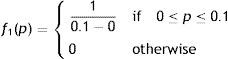
Number of defective items is in percentage p which is assumed to be a random variable having probability density function f1(p). The term p′ is the maximum percentage of imperfect quality items.
- •
Screening time to differentiate perfect and imperfect quality items is negligible. Screening cost is also negligible.
- •
System running time T is large in comparison to the preventive maintenance time t so that, during any time period T, buffer replenishment of perfect quality item starts from zero level.
- •
The regular preventive maintenance ensures that the probability of breakdown of the production unit during T is negligible, i.e., approximately zero.
- •
Before the starting of any normal preventive maintenance, the just-in-time buffer inventory for perfect quality inventory is Q1.
- •
Unused buffer inventory during t is depleted to zero during the next cycle time T.
- •
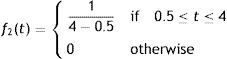
Regular preventive maintenance time t is a random variable having the probability density function f2(p).
- •
The buffer replenishment rate for perfect quality inventory is k1 unit per unit time.
- •
h1 and h2 are the holding cost per unit per unit time for perfect and imperfect quality items, respectively. Sp and Si are the shortage cost per unit for perfect and imperfect quality items, respectively.
- •
X(p, t) is the joint density function of p and t.
Under the just-in-time structure, the production unit produces both perfect and imperfect quality items. At the beginning of the preventive maintenance cycle to fulfill the demand of perfect quality items, the system produces perfect quality at rate D1 units per unit time. Since p% of produced items are defective, thus for the production of D1 units of perfect quality pD1/(1−p) units of imperfect quality items are produced. Toward the end of normal operation time T, the buffer inventory for perfect quality raises to Q1 at a rate k1 units per unit time. Thus total amount of buffer inventory for imperfect quality is pQ1/(1−p), which is replenished at a rate pk1/(1−p), units per unit time. However this finite replenishment starts Q1/k1 units time before the end of the time period T. At the end of time period T, the regular preventive maintenance starts and continues for a period of time t. The total system running cost involves holding cost and shortage cost for perfect and imperfect quality items (if we assume that the maintenance cost is fixed). We now calculate the expected unit total cost for perfect and imperfect quality items separately.
3.1Expected unit total cost for perfect quality inventoryFrom the beginning of the production cycle up to the time (T−Q1/k1), the perfect quality items are consumed immediately. The inventory is kept in stock for (Q1/k1) units of time in buffer through the replenishment at a rate k1 unit per unit time. Then, it is depleted during preventive maintenance. The behavior of inventory level is depicted in Fig. 1.

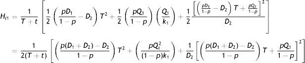
The average amount of perfect quality inventory during the time period (T+t) is
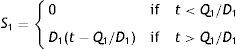
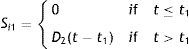
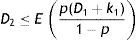
If the buffer supply time (Q1/D1) for perfect quality inventory is less than the preventive maintenance time t then shortages occur and the stock out time is (t−Q1/D1), otherwise stock out time is zero. Thus average shortage of perfect quality inventory per preventive maintenance cycle can be found as
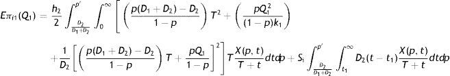
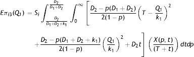
Therefore, the expected unit total cost for perfect quality inventory per preventive maintenance cycle is given by
3.2Expected unit total cost for imperfect quality inventory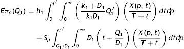
From the beginning of the production cycle, the demand of the imperfect quality is D2 units per unit time. Due to the production of D1 units of perfect quality items, amount of produced imperfect quality items is pD1/(1−p) units per unit time and it continues up to the time (T−Q1/k1). In the time interval T−Q1k1,T for the increment of buffer stock of perfect quality inventory at a rate k1 units per unit time, pk1/(1−p) units of imperfect quality items are produced per unit time up to the end of cycle time T. Now, the demand production relationship of imperfect quality items can be completely characterized by analyzing the following three cases:
Case 1: D2
Case 2: pD11−p
Case 3: pD11−p
In this case the demand of imperfect quality items D2 is less than the amount of imperfect quality items pD1/(1−p). Thus from the beginning of the production cycle after fulfilling the demand, the imperfect quality inventory level raises at a rate (pD1/(1−p)−D2) units per unit time up to the point of time (T−Q1/k1). Then, for the buffer stock additional k1 units of perfect quality, inventory is produced per unit time and imperfect quality items are produced at a rate [p(D1+k1)/(1−p)] per unit time for the time Q1/k1. Thus during the time period T−Q1k1,T, the inventory level raises at a rate p(D1+k1)1−p−D2 units per unit time. Here, the logistics diagram of inventory level is depicted in Fig. 2.
.")
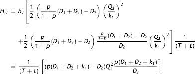
Total amount of inventory at the end of production cycle before the starting of preventive maintenance is pD11−p−D2T+Q1. During the preventive maintenance, it is depleted at a rate D2 units per unit time. Therefore, the average amount of imperfect quality items for the entire maintenance cycle is
If the preventive maintenance time t>1D2pD11−p−D2T+pQ11−p=t1, then shortages occur otherwise there is no shortage. Thus average shortage is
Hence, the expected unit total cost for imperfect quality inventory for the entire cycle in this case is
The demand of imperfect quality items, in this case, exceeds the amount of produced imperfect quality Items pD11−p per unit time. Thus there is shortage for imperfect quality items which is accumulated at a rate D2−pD11−p per unit time upto the time (T−Q1/k1). After that for the production of buffer inventory, imperfect quality items are produced at a rate p(D1+k1)1−p per unit time and D2
.")
And, the average amount of shortage is
where t2 is given by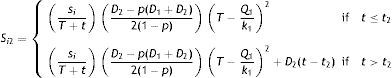
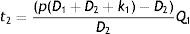
Hence, the expected unit total cost is given by
3.2.3Case-3: When pD11−p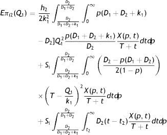
In this case, shortages occur for the entire preventive maintenance cycle. Therefore, the production of imperfect quality items during the time interval (0, T−Q1/k1) as well as in the time interval T−Q1k1,T are less than the demand of imperfect quality items D2. The behavior of inventory level is depicted in Fig. 4. Thus the holding cost is zero throughout the maintenance cycle. And, the average amount of shortage is
.")
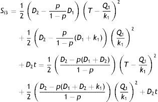
Therefore, the expected unit total cost is given by
The expected unit total cost of the system can be found as the sum of expected average holding cost and shortage cost of perfect quality and imperfect quality items, respectively, and is given by where


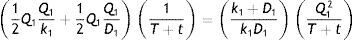
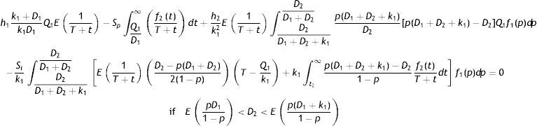
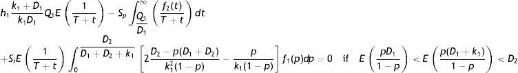
Eπp(Q1), Eπi1(Q1), Eπi2(Q1) and Eπi3(Q1) are given by Eqs. (1)–(4), respectively. It should be noted that X(p, t) is the joint density function of the percentage of defective items p and preventive maintenance time t. Since there is no inter-relationship between p and t, therefore, these two random variables are completely independent of each other and their joint density function can be expressed as the product of their individual density functions, i.e., X(p, t)=f1(p)f2(t). Our problem is to determine Q1 which minimizes Eπ(Q1). The necessary condition for this is dEπ(Q1)/dQ1=0. This yields after simplification as follows:
and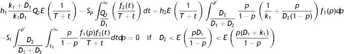
To evaluate the nature of the expected unit cost function Eπ(Q1), it is necessary to ascertain when the function is convex. But, it is difficult to verify that d2Eπ(Q1)/dQ12 is greater than zero to draw the conclusion about its convexity directly. Thus, an indirect approach is applied to verify the convexity of Eπ(Q1). A parametric study is carried out over the expected unit cost function for several values of Q1, and the response indicates that Eπ(Q1) is convex. However, it is difficult to derive a closed form solution for Q1. Only numerical solution can be obtained by using suitable numerical method. From the input values of the parameters, we have to calculate EpD11−p and Ep(D1+k1)1−p. If D2
Three different cost functions are derived above under three different scenarios arise for the control of imperfect quality items considering fixed buffer replenishment rate. In case-1, D2


However, in the decision making situation, verification is needed whether the increment of buffer replenishment rate beyond its capacity leads to diminish the expected unit system running cost or not. In case-2, shortage of imperfect quality items are continued from the beginning of the maintenance cycle upto the point of time (T−Q1/k1) and the imperfect quality items are stored in buffer from (T−Q1/k1) to T. By the same logic, for shortage instead of holding imperfect quality inventory, as in case-1, we can conclude that the shortage of imperfect quality items during [0, T−Q1/k1] cannot be avoided because it is uncontrollable. Only the holding cost of perfect and imperfect quality items may be reduced by adjusting the rate of production k1 of perfect quality items. Then, from the problem, we have as follows:


we have to determine Q1 and k1 and compare the cost with the fixed buffer replenishment rate. In case-3, shortage of imperfect quality items is accumulated throughout the preventive maintenance cycle because EpD11−p
However, it is worth mentioning that if the expected unit total system cost obtained by adjusting the buffer replenishment rate of perfect quality items, k1, is higher than that obtained for the fixed buffer replenishment rate, then, depending on the priority of preference, the decision maker will have to decide between minimum cost and loss of goodwill which will be selected. Otherwise, he will prefer to adjust the buffer replenishment rate. In the next section, we present a numerical example which may give some idea of these conflicting situations under decision making environment. The constraint optimization problems (11)–(13) are solved by using penalty function method.
4Numerical illustrationTo illustrate the proposed model, we consider a numerical example in which the parameter values are taken as T=30 days, D1=500units/day, h1=$0.4, h2=$0.1, Sp=$6, Si=$3. The percentage of imperfect quality items follows uniform distribution with the probability density function
The preventive maintenance time also follows uniform distribution with probability density function
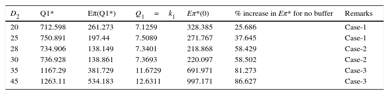
For fixed buffer replenishment rate, k1=100, the optimal buffer inventory for perfect quality items and corresponding expected unit total cost of the system are provided in Table 1. Eπ*(0) indicates the expected unit total cost of the system for a preventive maintenance cycle for no just-in-time buffer. The expected unit total cost for no just-in-time buffer is always higher than that with buffer inventory. It increases our strength of belief that proper just-in-time structure always requires some inventory for its efficient operation. The column (Q1/k1) indicates the required time for buffer replenishment. It is found that as the demand of imperfect quality items increases, the buffer replenishment time and the buffer stock increase. This is quite obvious because for higher demand during preventive maintenance larger amount of imperfect quality items is required. Eπ*(Q1) for D2=20, 25, 28, 30 and 35, 45 are obtained by solving Eqs. (8)–(10), respectively, depending on the relations between D2 and expected amount of imperfect quality items. It is found that Eπ*(Q1)|D2=35
Optimal values of Q1 and Eπ for Q1* and no buffer for fixed buffer replenishment rate (k1=100).
| D2 | Q1* | Eπ(Q1*) | Q1=k1 | Eπ*(0) | % increase in Eπ* for no buffer | Remarks |
|---|---|---|---|---|---|---|
| 20 | 712.598 | 261.273 | 7.1259 | 328.385 | 25.686 | Case-1 |
| 25 | 750.891 | 197.44 | 7.5089 | 271.767 | 37.645 | Case-1 |
| 28 | 734.906 | 138.149 | 7.3401 | 218.868 | 58.429 | Case-2 |
| 30 | 736.928 | 138.861 | 7.3693 | 220.097 | 58.502 | Case-2 |
| 35 | 1167.29 | 381.729 | 11.6729 | 691.971 | 81.273 | Case-3 |
| 45 | 1263.11 | 534.183 | 12.6311 | 997.171 | 86.627 | Case-3 |
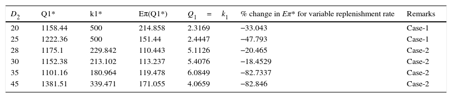
Optimal values of Q1, k1 and Eπ for variable buffer replenishment rate.
| D2 | Q1* | k1* | Eπ(Q1*) | Q1=k1 | % change in Eπ* for variable replenishment rate | Remarks |
|---|---|---|---|---|---|---|
| 20 | 1158.44 | 500 | 214.858 | 2.3169 | −33.043 | Case-1 |
| 25 | 1222.36 | 500 | 151.44 | 2.4447 | −47.793 | Case-1 |
| 28 | 1175.1 | 229.842 | 110.443 | 5.1126 | −20.465 | Case-2 |
| 30 | 1152.38 | 213.102 | 113.237 | 5.4076 | −18.4529 | Case-2 |
| 35 | 1101.16 | 180.964 | 119.478 | 6.0849 | −82.7337 | Case-2 |
| 45 | 1381.51 | 339.471 | 171.055 | 4.0659 | −82.846 | Case-2 |
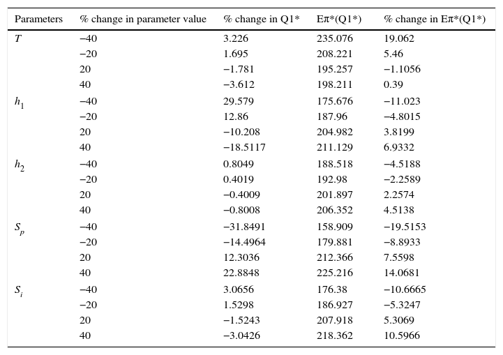
Sensitivity analysis for fixed buffer replenishment rate (for D2=25, k1=100).
| Parameters | % change in parameter value | % change in Q1* | Eπ*(Q1*) | % change in Eπ*(Q1*) |
|---|---|---|---|---|
| T | −40 | 3.226 | 235.076 | 19.062 |
| −20 | 1.695 | 208.221 | 5.46 | |
| 20 | −1.781 | 195.257 | −1.1056 | |
| 40 | −3.612 | 198.211 | 0.39 | |
| h1 | −40 | 29.579 | 175.676 | −11.023 |
| −20 | 12.86 | 187.96 | −4.8015 | |
| 20 | −10.208 | 204.982 | 3.8199 | |
| 40 | −18.5117 | 211.129 | 6.9332 | |
| h2 | −40 | 0.8049 | 188.518 | −4.5188 |
| −20 | 0.4019 | 192.98 | −2.2589 | |
| 20 | −0.4009 | 201.897 | 2.2574 | |
| 40 | −0.8008 | 206.352 | 4.5138 | |
| Sp | −40 | −31.8491 | 158.909 | −19.5153 |
| −20 | −14.4964 | 179.881 | −8.8933 | |
| 20 | 12.3036 | 212.366 | 7.5598 | |
| 40 | 22.8848 | 225.216 | 14.0681 | |
| Si | −40 | 3.0656 | 176.38 | −10.6665 |
| −20 | 1.5298 | 186.927 | −5.3247 | |
| 20 | −1.5243 | 207.918 | 5.3069 | |
| 40 | −3.0426 | 218.362 | 10.5966 | |
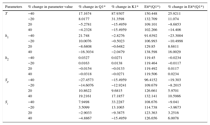
Sensitivity analysis for variable buffer replenishment rate (for D2=35).
| Parameters | % change in parameter value | % change in Q1* | % change in K1* | Eπ*(Q1*) | % change in Eπ*(Q1*) |
|---|---|---|---|---|---|
| T | −40 | 17.1674 | 87.9307 | 150.448 | 25.9211 |
| −20 | 8.0177 | 31.3598 | 132.709 | 11.074 | |
| 20 | −5.2781 | −15.4959 | 109.101 | −8.6853 | |
| 40 | −4.2328 | −15.4959 | 102.266 | −14.406 | |
| h1 | −40 | 21.748 | −2.8276 | 91.6392 | −23.3004 |
| −20 | 10.0076 | −0.5023 | 106.993 | −10.4998 | |
| 20 | −8.6808 | −0.6482 | 129.85 | 8.6811 | |
| 40 | −16.3034 | −2.0479 | 138.598 | 16.0029 | |
| h2 | −40 | 0.0327 | 0.0271 | 119.45 | −0.0234 |
| −20 | 0.0163 | 0.0138 | 119.464 | −0.0117 | |
| 20 | −0.0154 | −0.0133 | 119.492 | 0.0117 | |
| 40 | −0.0318 | −0.0271 | 119.506 | 0.0234 | |
| Sp | −40 | −27.4573 | −15.4959 | 96.4152 | −19.303 |
| −20 | −14.6076 | −12.9241 | 109.679 | −8.2015 | |
| 20 | 10.8622 | 9.6815 | 126.661 | 5.9701 | |
| 40 | 19.2161 | 17.1857 | 132.141 | 10.5986 | |
| Si | −40 | 7.9498 | 33.2287 | 108.676 | −9.041 |
| −20 | 3.5099 | 13.1065 | 114.738 | −3.9673 | |
| 20 | −2.9033 | −9.3875 | 123.363 | 3.2516 | |
| 40 | −4.8867 | −15.4959 | 126.656 | 6.0078 | |
In the existing literature, plenty of maintenance policies and inspection policies are available to cope with the production of imperfect quality items for imperfect repair during preventive maintenance and for the production of imperfect quality items due to the out-of-control state of the production unit. But, in this paper, we developed a model under the basic assumption that the system produces imperfect quality items or produces items not to the standard maintained by the production unit in random proportion due to some uncontrollable factors of production (frequently found to happen in polymer, cotton and leather industries) and completely independent of the nature of the preventive maintenance under the just-in-time configuration.
Quite often, it is observed in polymer, cotton and leather industries that a percent of the finished goods are defective due to imperfect operations at any stage of the production processes. The items are marked imperfect, after screening process, in respect of quality factors for branding such as quality of materials, colors, accurate shape and size, sewing, etc. These imperfect, i.e., defective items are purchased at lower price compared to the perfect quality items at the secondary shops/enterprises.
It is also assumed that, after preventive maintenance, the quality of the products remains same as before. The optimal just-in-time buffer for perfect and hence imperfect quality items are determined by considering fixed buffer replenishment rate and variable buffer replenishment rate beyond its capacity to minimize expected unit system running cost. A numerical example is presented which illustrates that, in just-in-time structure; some buffer inventory must be needed to minimize the system running cost. The demand of imperfect quality items has a significant effect on the expected system running cost. It is also found that the adjustment of buffer replenishment rate beyond its capacity depending on the expected amount of imperfect quality items leads to lower system running cost than the predetermined fixed buffer replenishment rate. In the decision making context, for lower demand of imperfect quality items in comparison to the demand of perfect quality items, it is always better to adjust the buffer replenishment rate. However, it is assumed that T is fixed. An interesting area of further investigation is to determine T, k1 and Q1 simultaneously which would be generalization of the model presented here. This also determines the joint effects of unavoidable random amount of imperfect quality items and the imperfect quality items produced due to the out-of-control state of the production unit on the expected unit system running cost. The paper provides an elementary idea about how production of perfect quality product is affected by imperfect quality product which is produced due to error in the production unit. In the current business era, imperfect quality product has a good demand. Thus, further investigation is essential to obtain maximum benefit from this market through proper inventory policies for imperfect quality product.
