
Edited by: Brij B. Gupta, Kwok Tai Chui
Last update: July 2022
More infoBased on the real-world knowledge innovation management characteristics of enterprises, in this paper a novel bilateral matching (BM) decision-making method for knowledge innovation management considering the matching willingness of bilateral enterprises is proposed. The method uses interval-valued intuitionistic fuzzy sets (IvIFSs) as its basis. First, using the IvIFS preferences of the bilateral enterprises, their matching willingness is calculated according to the TOPSIS method. Then, the BM model is constructed according to the IvIFS preference, the matching willingness and the BM matrix of the bilateral enterprises. According to the normalized interval-valued score function (NIvSF) and score function (SF), the BM model is transformed into a BM model with SFs. Considering the fairness of each agent of each side, the BM model with SFs is transformed into a two-objective BM model. Furthermore, a novel optimization algorithm is introduced to solve the two-objective model, and then the optimal BM scheme is obtained. Finally, the effectiveness and feasibility of the proposed method are verified by a knowledge innovation management case study. The key findings of the proposed work are as follows: (1) The proposed method establishes the BM model with IvIFSs and matching willingness; (2) a new algorithm for the BM model is developed; and (3) the obtained BM scheme using the proposed method reflects the matching willingness of the agents. The proposed method can be extended to other BM problems in knowledge innovation management operating under other intuitionistic fuzzy environments and can be applied to other decision-making problems in enterprise knowledge innovation management.
Bilateral matching (BM) belongs within the research realm of decision-making. BMs have been investigated and applied in different fields, such as the volunteer assignment of emergency tasks (Chen, Zhang, Shi & Wang, 2021), random stable matching (Pittel, 2020), heterogeneous workers-entrepreneurs matching (Choi, 2020), configuring cloud manufacturing tasks and resources (Li, Yang, Su, Liang & Wang, 2020), venture capitalist and firm matching (Antón & Dam, 2020), managing competition (Belleflamme & Peitz, 2019; Ribeiro & Golovanova, 2020), etc. Gale and Shapley (1962) first studied two renowned BM problems with ordinal preferences. According to the aforementioned reference, it is well known that the BM mainly concentrates on acquiring the appropriate BM scheme according to the preferences of the agents. After the initial study, a variety of BM theories were proposed (Kadadha, Otrok, Singh, Mizouni & Ouali, 2021; Kadam & Kotowski, 2018; Lazarova & Dimitrov, 2017; Li, Zhang & Xu, 2020; Wang, Chen & Wu, 2019; Zhang, Gao, Gao & Yu, 2021); some deformations and applications for BM were extended (Shu, Cai & Xiong, 2021; Xie, Wang & Miao, 2021; Zhang, Kou, Palomares, Yu & Gao, 2019). Hence, the research on BM is meaningful in theory and valuable in practice.
Currently, due to the complexity of the social environment, uncertainty of cognition, and the fuzziness of judgements, the preference information for practical problems is not usually in the form of exact values, but rather in the form of intuitionistic fuzzy sets (IFSs) (Düğenci, 2016). Interval-valued intuitionistic fuzzy sets (IvIFSs) (Atanassov & Gargov, 1989) are treated as the popularization of IFSs, and better reflect the uncertainty of human judgement because of the degrees of interval membership, interval non-membership and interval hesitancy. Therefore, studying BM with IvIFS preferences also has significant research significance.
With the development of the social economy and the changes in organizational management, knowledge management has become a form of management innovation. Knowledge management mainly refers to the management of people, organizations and technologies, emphasizing an organic combination of managing the wealth of knowledge embedded in employees and organizations and the application of information technology to exploit the knowledge innovation and value creation of enterprises. Compared with knowledge management, knowledge innovation management focuses on the management of people and encourages people to create, share and use knowledge effectively. Knowledge is the core economic resource and intellectual capital of enterprises. Effective knowledge management can improve an enterprise's performance. With respect to knowledge innovation management, Kamasak and Bulutlar (2010) discussed the impact of two different forms of knowledge sharing, including knowledge donation and knowledge collection. Carneiro (2000) proposed a conceptual model that focuses on the relationships between knowledge management, competitiveness and innovation, which emphasized the importance of knowledge development and the role of knowledge management in ensuring competitiveness. Furthermore, for the critical knowledge service link in knowledge management, Chen, Li, Fan, Zhou and Zhang (2016) considered the expected level of the attributes given by demanders and suppliers and proposed a method to match the appropriate knowledge service demanders and suppliers. Considering the difference between the digital platform service mode and the traditional service mode in knowledge services, Chang, Li and Sun (2019) proposed a new method to match knowledge suppliers and demanders on digital platforms. Han, Li, Liang and Lai (2018) proposed a BM method between technical knowledge suppliers and demanders that considered the characteristics of the supply-demand network.
A large number of studies on IvIFSs have emerged in many research areas. First, the theory of IvIFS has been generalized, as reflected in the generalized Dice measure (Ye, 2018), distance measure (Düğenci, 2016; Liu & Jiang, 2020), ranking (Nayagam & Sivaraman, 2011), knowledge measure (Das, Dutta & Guha, 2016; Guo & Zang, 2019), entropy (Mishra et al., 2020; Wei, Wang & Zhang, 2011), divergence measure (Mishra et al., 2020; Mishra, Chandel & Motwani, 2020), operator (Deschrijver & Kerre, 2005; Zindani, Maity & Bhowmik, 2020), score function (Wang & Chen, 2017, 2018), and so on. Second, the application scope of IvIFS has expanded. For example, a multiattribute decision-making (MADM) method for IvIFSs using set pair analysis (SPA) theory is available (Garg & Kumar, 2020). A new framework and the latest aggregation method for implementing multiattribute group decision-making based on the concepts of TODIM, WASPAS and TOPSIS under interval-valued intuitionistic fuzzy uncertainty have been developed (Davoudabadi, Mousavi & Mohagheghi, 2020). With respect to the interval-valued intuitionistic fuzzy group decision-making problem with incomplete attribute weight information, Wan and Dong (2020) directly used the constant vector as the attribute weight to solve the decision-making problem. Considering the complexity of the decision-making environment, Liu, Yu, Chan and Niu (2021) proposed a group decision-making method based on interval intuitionistic fuzzy sets by integrating the variable weight, correlation coefficient and similarity ranking technology with an ideal solution. Based on the proposed connection number score function (SF) and SPA theory, a new MADM method in an interval-valued intuitionistic fuzzy environment was proposed (Kumar & Chen, 2021). A group decision-making model for project delivery system selection was proposed by using IvIFS theory, which can aid project owners in project delivery system selections (An, Wang, Li & Ding, 2018). A new MADM method based on the U-quadratic distribution of intervals and the transformed matrix of the decision matrix in an interval-valued intuitionistic fuzzy environment was proposed, which overcomes the shortcomings of the existing MADM methods (Chen & Chu, 2020).
However, to the best of our knowledge, there is little research on the theory and method of IVFSs in the field of BM. For instance, two new similarity measures between triangular intuitionistic fuzzy numbers were displayed, which were used to develop the corresponding decision-making approaches for BM problems under a triangular intuitionistic fuzzy environment (Yue, Zhang, Yu, Zhang & Zhang, 2019). The problem of machine position matching in intelligent production lines was solved from the perspective of position uniformity, and an interval-valued intuitionistic fuzzy BM method considering the automation level was proposed (Liang, Yang & Liao, 2022). An intuitionistic fuzzy Choquet integral aggregation operator-based two-sided matching model was developed, which can effectively solve personnel-position matching problems with correlated evaluated attributes (Yu & Xu, 2019). In addition, the theory and method of IvIFSs are less studied than those of IFSs. For instance, a decision-making method was presented for solving the BM problem with IvIFSs and matching aspirations (Yue et al., 2016). An interval-valued intuitionistic fuzzy two-sided matching decision-making approach was proposed, in which agents' behaviours are considered (Yue & Zhang, 2020). Nevertheless, the proposed interval-valued scores in Yue et al. (2016) could be less than 0. The method proposed in Yue and Zhang (2020) is actually based on interval-valued intuitionistic fuzzy numbers (IvIFNs) rather than IvIFSs. The matching aspiration proposed by Yue et al. (2016) and Yue and Zhang (2020) is also based on IvIFNs rather than on IvIFSs.
The main ideas contained in this paper are as follows: First, the TOPSIS method is used to calculate the matching willingness of the bilateral agents directly based on IvIFS preferences, which leverages information as much as possible. Then, the BM model is constructed according to the IvIFS preference and matching willingness, a method that has been ignored by some scholars. Moreover, the normalized interval-valued score function (NIvSF) and SF are introduced. On this basis, a new optimization algorithm is used to solve the model and obtain the optimal BM scheme, providing new solution possibilities.
Motivated by the aforementioned ideas, this paper investigates the BM problem with IvIFSs from the view of matching willingness to obtain more reasonable formulas of matching willingness and a more effective BM scheme. The key contributions of this work are as follows: (1) Two effective computational algorithms for matching willingness in the IvIFS environment are proposed. (2) A BM model using IvIFSs and matching willingness is demonstrated. (3) An effective algorithm for solving the demonstrated BM model using the NIvSFs is developed. (4) An algorithm for solvingthe BM problem on the basis of IvIFSs and matching willingnessis given. (5) A sensitivity analysis of the proposed algorithm is conducted. Compared with previous studies, two effective computational algorithms for obtaining the matching willingness of bilateral agents are given based on the TOPSIS method; the method has a stronger theoretical foundation and is more helpful to improve the satisfaction of the bilateral agents. In addition, the proposed algorithm using NIvSFs to solve the BM model is also a new attempt, which can be extended to multiple intuitionistic fuzzy set decision-making environments. Finally, the developed algorithm for solving the BM problem with IvIFS and matching willingness is novel, which enriches the research of relevant methods.
The remaining structure of this paper is as follows. Section 2 explores some concepts of IvIFS and BM. Section 3 presents the BM problem for IvIFSs considering matching willingness. Section 4 proposes the BM decision-making method with IvIFSs using the TOPSIS technology. Section 5 uses a BM case study in knowledge innovation management to reveal the effectiveness and feasibility of the proposed method. Section 6 discusses the sensitivity of the BM case. Section 7 summarizes this paper.
PreliminariesIvIFSDefinition 1 (Atanassov & Gargov, 1989): Assume G is a limited domain; then, an IvIFS is defined by F¯={
Definition 2 (Atanassov & Gargov, 1989): Assume hF¯(x)=[1,1]−pF¯(x)−qF¯(x); then, hF¯(x)=[hF¯L(x),hF¯R(x)] stands for the interval-valued hesitancy degree.
In particular, when pF¯(x)+qF¯(x)=[1,1], F¯ degenerates into a conventional fuzzy set. For convenience, an IvIFS F¯={
The following arithmetic rule of IvIFN is employed.
Definition 3 (Xu & Chen, 2007): Assuming f¯1= f¯1+f¯2=<[pF¯1L+pF¯2L−pF¯1LpF¯2L,pF¯1R+pF¯2R−pF¯1RpF¯2R],[qF¯1LqF¯2L,qF¯1RqF¯2R]>, f¯1×f¯2=<[pF¯1LpF¯2L,pF¯1RpF¯2R],[qF¯1L+qF¯2L−qF¯1LqF¯2L,qF¯1R+qF¯2R−qF¯1RqF¯2R]>, lf¯1=<[1−(1−pF¯1L)l,1−(1−pF¯1R)l],[(qF¯1L)l,(qF¯1R)l]>,l>0, (f¯1)l=<[(pF¯1L)l,(pF¯1R)l]],[1−(1−qF¯1L)l,1−(1−qF¯1R)l]>,l>0, (f¯1)c=<[qF¯1L,qF¯1R],[pF¯1L,pF¯1R]>.
Definition 4 (Xu & Chen, 2007): Assume f¯1=<[pF¯1L,pF¯1R],[qF¯1L,qF¯1R]>, f¯2=<[pF¯2L,pF¯2R],[qF¯2L,qF¯2R]>,...,f¯l=<[pF¯lL,pF¯lR],[qF¯lL,qF¯lR]> is the l collection of IvIFNs. Let IvIFWA:Ψ¯n→Ψ¯ if the following formula holds:
where w=(w1,w2,...wl) is the weight vector of (f¯1,f¯2,...,f¯l) and has nonnegativity and normalization; then, IvIFWAw(f¯1,f¯2,...,f¯l) is referred to as an interval-valued intuitionistic fuzzy weighted averaging operator.In Definition 4, if w1,w2,...wl are equal, then the above operator is simplified as an interval-valued intuitionistic fuzzy averaging operator and is exhibited as follows:
Definition 5 (Xu & Chen, 2007): Assume f¯1=<[pF¯1L,pF¯1R],[qF¯1L,qF¯1R]>, f¯2=<[pF¯2L,pF¯2R],[qF¯2L,qF¯2R]>,...,f¯l=<[pF¯lL,pF¯lR],[qF¯lL,qF¯lR]> is the l collection of IvIFNs. Let IvIFWG:Ψ¯n→Ψ¯, if the following formula holds:
where w=(w1,w2,...wl) is the weight vector of (f¯1,f¯2,...,f¯l) and meets the criteria for nonnegativity and normalization; then, IvIFWGw(f¯1,f¯2,...,f¯l) is referred to as an interval-valued intuitionistic fuzzy weighted geometric operator.In Definition 5, if w1,w2,...wl are equal, then the above operator is simplified as an interval-valued intuitionistic fuzzy geometric operator and is exhibited as follows:
NIvSFAccording to Yue et al. (2016), the following definition of NIvSF is used.
Definition 6: Assume f¯=
In this subsection, a novel distance measure for IvIFSs, which is an extension of that proposed in Düğenci (2016) and Boran and Akay (2014), is developed.
Definition 7: Assume F¯1={f¯F¯11,f¯F¯12,...,f¯F¯1n} and F¯2={f¯F¯21,f¯F¯22,...,f¯F¯2n} are two IvIFSs, where f¯F¯1k=
The following mathematical symbols for the BM problem are employed in this paper. Let χ={χ1,χ2,...,χm} and γ={γ1,γ2,...,γn} be two separate sets of agents. Here, χj and γk represent the jth and the kth agents on each side. Let M={1,...,m}, N={1,...,n}, and 2≤m≤n.
Definition 8 (Yue & Zhang, 2020): Assume Λ:χ∪γ→χ∪γ is a one-one mapping. If the mapping Λmeets these conditions, i) Λ(χj)∈γ, ii) Λ(γk)∈χ∪{γk}, iii) Λ(χj)=γk if Λ(γk)=χj, then Λ is called a BM.
In Definition 8, Λ(χj)=γk indicates that Λ(χj,γk) is a matching pair, and Λ(γk)=γk indicates that Λ(γk,γk) is a single matching pair.
Definition 9 (Yue & Zhang, 2020): For BM Λ:χ∪γ→χ∪γ, another form is Λ=ΛM∪ΛS, where ΛM is the set of matching pairs, and ΛS is the set of single matching pairs.
BM problem for IvIFSs considering matching willingnessLet F¯jχ={
Remark 1 Matching willingness wjχ and wkγ can be acquired in accordance with the theory of TOPSIS. Two algorithms will be introduced in the next section.
In summary, this paper shall investigate how to obtain the optimum BM Λ*=ΛM*∪ΛS* in accordance with IvIFSs F¯jχ and F¯kγ, and matching willingness wjχ and wkγ. To acquire the optimum BM, the related concepts and theories of IvIFS and BM will be adopted in Section 2 and then displayed in Section 4 in detail. The chief notations and acronyms for this paper are shown in Table 1.
Notations and acronyms.
The procedures of the proposed BM decision-making method with IvIFSs and matching willingness are given as follows. First, the matching willingness is computed through Algorithm 1 and Algorithm 2. Then, the IvIFS BM model considering the matching willingness is constructed through the multiobjective programming method. Third, the BM model is transformed into a biobjective BM model using NIvSF and SF. Finally, the optimal BM scheme is obtained through Algorithm 3. (Fig. 1)
Computation of matching willingnessIn Section 3, the matching willingness wjχ and wkγ are unknown. This subsection will introduce two approaches to determine them. The procedures of Algorithm 1 for determining wjχ are displayed below.
Algorithm 1:
Input: IvIFS F¯jχ={
Step 1: Compute the positive-ideal IvIFS of side χ, i.e., F¯j*χ={
Step 2: Compute the negative-ideal IvIFS of side χ, i.e., F¯j∘χ={
Step 3: Calculate the positive distance between F¯jχ={
Step 4: Calculate the closeness degree cjχ of χj, where cjχ is computed by:
Step 5: Calculate the matching willingness wjχ of χj, where wjχ is computed by:
Output: Matching willingness of χj, i.e., wjχ.
Similarly, the procedures of Algorithm 2 for determining wkγ are displayed below.
Algorithm 2:
Input: IvIFS F¯kγ={
Step 1: Compute the positive-ideal IvIFS of side γ, i.e., F¯k*γ={
Step 2: Compute the negative-ideal IvIFS of side χ, i.e., F¯k∘γ={
Step 3: Calculate the positive distance between F¯kγ={
Step 4: Calculate the closeness degree ckγ of γk, where ckγ is computed by:
Step 5: Calculate the matching willingness wkγ of γk, where wkγ is computed by:
Output: Matching willingness of γk, i.e., wkγ.
From the above descriptions, Algorithm 1 is divided into five steps, which do not require many computations. The computational complexity is as follows: Step 1 requires only n Max operations; Step 2 requires only n Min operations; Step 3 requires no more than 21n2 operations; Step 4 requires only 2n operations; Step 5 requires no more than 2n operations. The complexity of the computation of Algorithm 2 is the same as that of Algorithm 1. Furthermore, the matching willingness of the bilateral agents can be determined through Algorithm 1 and Algorithm 2.
Construction of the BM modelFirst, the BM variable vjk is introduced, i.e.,
Consequently, a BM matrix V=[vjk]m×n can be established. In accordance with IvIFSs F¯jχ={To solve Model (16), IvIFNs
Remark 2 From Yue et al. (2016), it is realized that αF¯jχk can be treated as the support ratio of Λ(χj)=γk from side χ, and αF¯kγj can be treated as the support ratio of Λ(χj)=γk from side γ.
Then, NIvSFs [sF¯jχk,L,sF¯jχk,R] and [sF¯kγj,L,sF¯kγj,R] are transformed into SFs sF¯jχk and sF¯kγj, where:
In Eqs. (19) and (20), θF¯jχk stands for the optimism attitude of χj towards γk, and θF¯kγj stands for the optimism attitude of γk towards χj. Through Eqs. (17)-(20), we know that a higher IvIFN satisfaction corresponds to a larger score, and vice versa. Moreover, the BM Model (16) can be changed into the following BM Model (21) with SFs, where the model constraint is still the one-to-one quantitative matching.
Ordinarily, the priorities of the agents of each side are treated as the same. From this point, the BM Model (21) can be translated into a biobjective BM Model (22):
To solve the above biobjective BM Model (22), a new optimization algorithm is introduced. The ideas of the new algorithm are as follows: First, solve the maximum and minimum values of a single objective function in Model (22) under the same constraints. Then, we transform Model (22) into a single objective model according to the idea of obtaining as much satisfaction as possible. The procedures of the new optimization algorithm are exhibited below.
Algorithm 3:
Input: SFs sF¯jχk and sF¯kγj.
Step 1: Find the maximum value Bχmax through the solution of BM Model (23):
Step 2: Find the minimum value Bχmin through the solution of BM Model (24):
Step 3: Find the maximum value Bγmax through the solution of BM Model (25):
Step 4: Find the minimum value Bγmin through the solution of BM Model (26):
Step 5: Transform the BM Model (22) into the following BM Model (27) in accordance with the idea of the new optimization algorithm:
Output: Maximum values Bχmax and Bγmax, minimum values Bχmin and Bγmin.
From the above description, it is also known that Algorithm 3 consists of five steps, and its calculation is more complex than Algorithm 1 or Algorithm 2, as shown below. The implementation process of Step 1 of Model (23) shall not exceed 2mn iterations, which is the same as the other steps.
Remark 4 If the priority of the agent of sides χ and γ is not the same, AHP technology can be used to acquire the priority of the agent of each side.
In summary, the BM decision-making Model (22) with SFs can be solved through Algorithm 3, and then the optimal BM matrix V*=[vjk*]m×n is obtained.
Procedure for the BM method based on IvIFSs and matching willingnessIn this section, a novel method for solving the BM problem on the basis of IvIFSs and matching willingness is exhibited.
Step 1: Find matching willingness wjχ through the use of Algorithm 1.
Step 2: Find matching willingness wkγ through the use of Algorithm 2.
Step 3: Construct the BM Model (16) in accordance with IvIFSs F¯jχ and F¯kγ, matching willingness wjχ and wkγ, and the BM matrix V=[vjk]m×n.
Step 4: Transform IvIFN
Step 5: Transform IvIFN
Step 6: Transform NIvSFs [sF¯jχk,L,sF¯jχk,R] and [sF¯kγj,L,sF¯kγj,R] into SFs sF¯jχk and sF¯kγj through the use of Eqs. (19) and (20), respectively.
Step 7: Convert BM Model (16) into BM Model (21).
Step 8: Convert BM Model (21) into the biobjective BM Model (22).
Step 9: Transform BM Model (22) into BM Model (27) through the use of new optimization.
Step 10: Gain the optimal BM scheme through the solution of Model (27).
A BM case study for knowledge innovation management in the IvIFS environmentA BM case study in the field of knowledge innovation management shows the feasibility of the presented decision-making method.
A technology service company for a knowledge management system in Shenzhen provides cross-industry knowledge management system purchase, customization and matching services for suppliers and demand enterprises through its service platform. At present, the company's service platform has received the purchase intention of five enterprises χ1,χ2,...,χ5 to purchase a knowledge management system in advance to improve the efficiency of their internal knowledge management and meet their long-term needs. During this period, six suppliers γ1,γ2,...,γ6 on the platform expressed their trading intention. Five enterprises χ1,χ2,...,χ5 evaluate six suppliers γ1,γ2,...,γ6 mainly from the aspects of system performance, purchase price and after-sales service and then give the preference of IvIFS, F¯jχ={
IvIFS preferences F¯jχ={
IvIFS preferences F¯kγ={
To provide enterprises and suppliers with a more effective BM scheme, a calculation process is described according to the IvIFS preferences F¯jχ (j=1,2,...,5) and F¯kγ (k=1,2,...,6), which are the original input values.
Step 1: Find matching willingness wjχ(j∈M={1,...,5}) through the use of Algorithm 1. The uncomplicated calculation procedures are revealed below.
Algorithm 4:
Input: IvIFS F¯jχ (j=1,2,...,5).
Step 4.1: Gain the positive-ideal IvIFS F¯j*χ={
Step 4.2: Gain the negative-ideal IvIFS F¯j∘χ={
Step 4.3: Obtain the positive distance Dj*χ between F¯jχ(j∈M) and F¯j*χ and the negative distance D∘jχ between F¯jχ(j∈M) and F¯j∘χ through the use of Eq. (7), where r,α,β,γ=1,0.4,0.4,0.2.
Step 4.4: Gain closeness degree cjχ(j∈M) through the use of Eq. (10).
Step 4.5: Gain matching willingness wjχ(j∈M), i.e., w1χ=0.1815, w2χ=0.1765, w3χ=0.2758, w4χ=0.1599, w5χ=0.2063.
Output: Matching willingness wjχ (j=1,2,...,5).
Step 2: Determine the matching willingness wkγ(k∈N={1,...,6}) through the use of Algorithm 2. The uncomplicated calculation procedures are revealed below.
Algorithm 5:
Input: IvIFS F¯kγ (k=1,2,...,6).
Step 5.1: Gain the positive-ideal IvIFS F¯k*γ={
Step 5.2: Gain the negative-ideal IvIFS F¯k∘γ={
Step 5.3: Obtain the positive distance Dk*γ(k∈N) between F¯kγ(k∈N) and F¯k*γ and the negative distance Dk∘γ(k∈N) between F¯kγ(k∈N) and F¯k∘γ through the use of Eq. (7), where r,α,β,γ=1,0.4,0.4,0.2.
Step 5.4: Gain closeness degree ckγ(k∈N) through the use of Eq. (14).
Step 5.5: Gain matching willingness wkγ(k∈N), i.e., w1γ=0.145, w2γ=0.1662, w3γ=0.173, w4γ=0.1411, w5γ=0.1778, w6γ=0.1969.
Output: Matching willingness wkγ (k=1,2,...,6).
Step 3: Construct the following BM Model (16) in accordance with IvIFSs F¯jχ(j∈M) and F¯kγ(k∈N), matching willingness wjχ(j∈M) and wkγ(k∈N), and the BM matrix V=[vjk]5×6:
whereStep 4: Transform IvIFN
NIvSF [sF¯jχk,L,sF¯jχk,R].
Step 5: Transform IvIFN
NIvSF [sF¯kγj,L,sF¯kγj,R].
Step 6: Transform NIvSFs [sF¯jχk,L,sF¯jχk,R] and [sF¯kγj,L,sF¯kγj,R] into SFs sF¯jχk and sF¯kγj through the use of Eqs. (19) and (20), respectively, as demonstrated in Table 8 and Table 9 with θF¯jχk=θF¯kγj=0.6.
Step 7: Convert BM Model (16) into BM Model (21) in accordance with SFs sF¯jχk and sF¯kγj, i.e.,
Step 8: Convert BM Model (21) into the biobjective BM Model (22) under normal circumstances, i.e.,
Step 9: Transform BM Model (22) into BM Model (27) through the use of Algorithm 3. The calculation procedures are revealed below.
Algorithm 6:
Input: SFs sF¯jχk and sF¯kγj (j=1,2,...,5; k=1,2,...,6).
Step 6.1: Solve the BM Model (23); then maximum value Bχmax is gained, i.e., Bχmax=0.7293.
Step 6.2: Solve the BM Model (24); then minimum value Bχmin is gained, i.e., Bχmin=0.5823.
Step 6.3: Solve the BM Model (25); then maximum value Bγmax is gained, i.e., Bγmax=0.6238.
Step 6.4: Solve the BM Model (26): then minimum value Bγmin is gained, i.e., Bγmin=0.4767.
Step 6.5: Transform the BM Model (22) into the following BM Model (27) in accordance with the calculation results of Steps 6.1–6.4, i.e.,
Output: Maximum values Bχmax and Bγmax, minimum values Bχmin and Bγmin.
Step 10: By solving Model (27), we can acquire the optimal objective function value θχ*+θγ*=1+0.6179=1.6179 and the optimal BM matrix V=[vjk*]5×6, as demonstrated in Table 10.
As a result, the optimal BM scheme Λ* is gained, Λ*=ΛM*∪ΛS*, where ΛM*={(χ1,γ3),(χ2,γ6),(χ3,γ5),(χ4,γ2),(χ5,γ1)}, ΛS*={(γ4,γ4)}.
Remark 5 It should be emphasized that the decision-making method proposed in this paper is based on IvIFSs. However, the methods proposed in Yue et al. (2016) and Yue and Zhang (2020) were actually based on IvIFNs rather than IvIFSs, which cannot be used to directly solve the IvIFS BM problem displayed in this paper. The proposed decision-making method uses the distance measure for IvIFSs directly for calculating the matching willingness of the bilateral agents, which can reduce information loss. The proposed decision-making method solves the BM problem under the fuzzy background of IvIFS by building the BM model considering the matching willingness of the bilateral agents. It not only expands the solution approach of the BM problem in knowledge innovation management under the IvIFS environment but also provides a reference for solving the BM problem and other decision-making problems considering the matching willingness under other intuitionistic fuzzy environments.
If the priorities of agents of sides χ and γ are not the same, then let ωχ and ωγ be the weights of agents of side χ and γ, respectively. Moreover, the objective function of Model (27) is turned into f=ωχθχ+ωγθγ. As a result, Model (27) is translated into the following BM model:
Different values of parameters ωχ and ωγ are discussed below. Several different situations of f are displayed in Table 11. To reflect the impact on the experimental results, the different priorities of the bilateral agents in the process of BM decision-making are analysed (Chui, Liu, Zhao & Pablos, 2020). We will discuss the relationships among parameters ωχ and ωγ, objective function f=ωχθχ+ωγθγ, SFs sF¯jχk and sF¯kγj and the optimal BM matrix V=[vjk*]5×6.Several different situations of f=ωχθχ+ωγθγ.
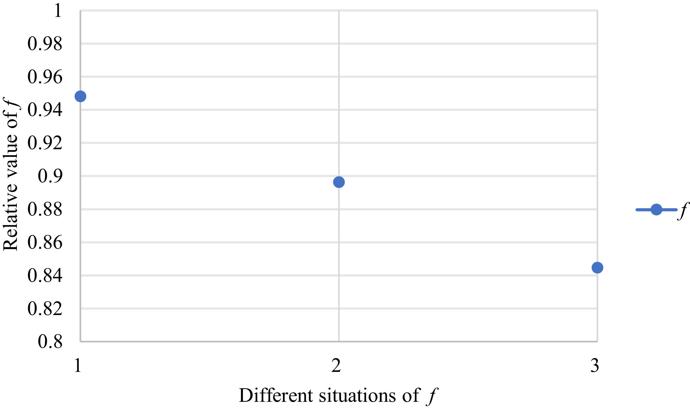
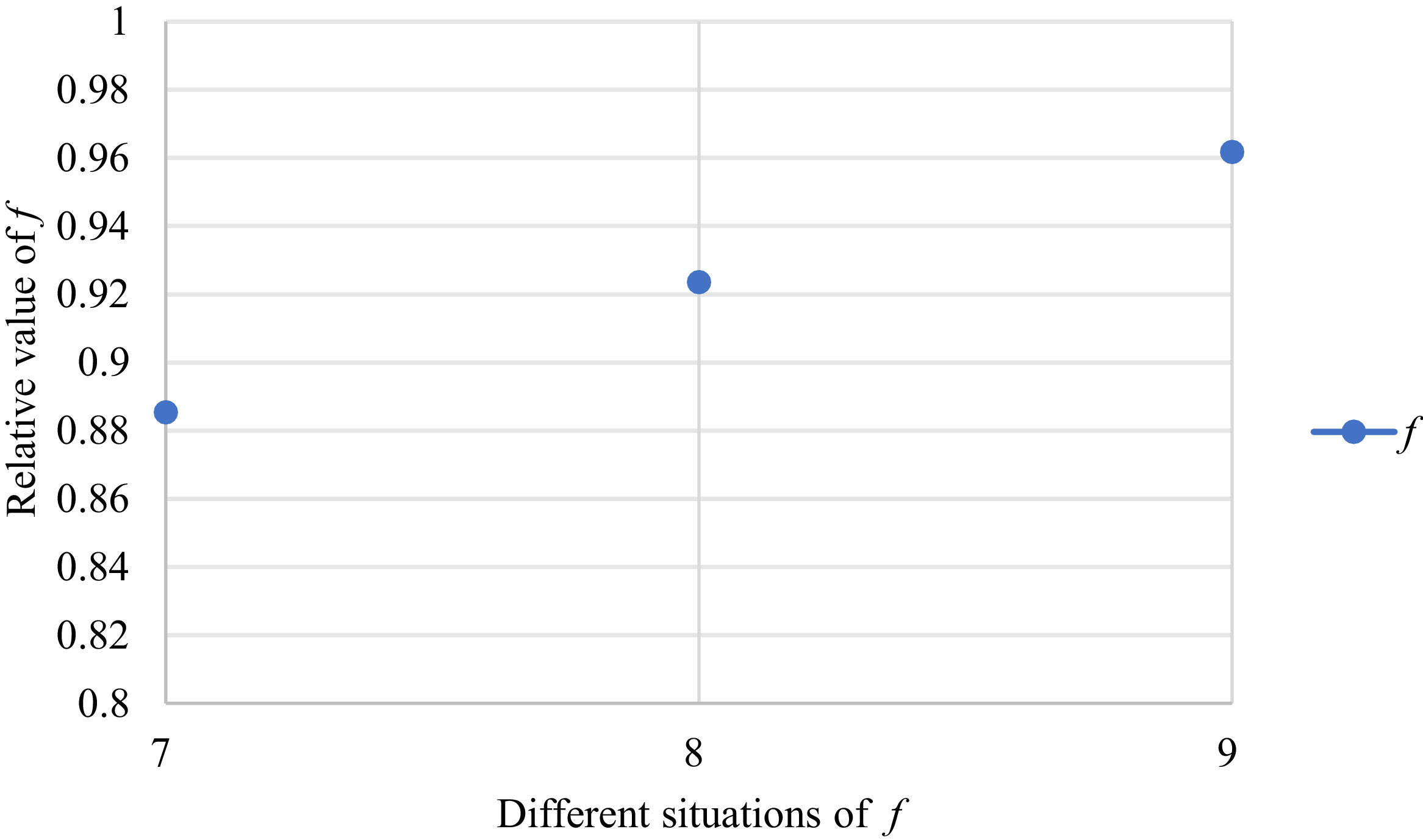
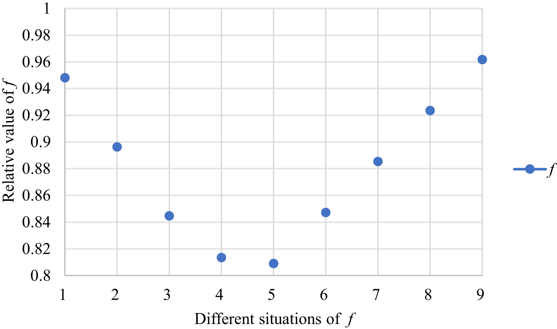
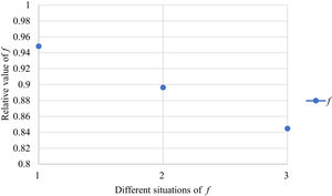
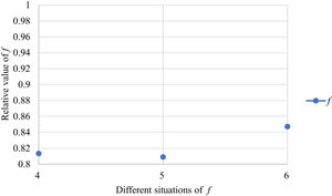
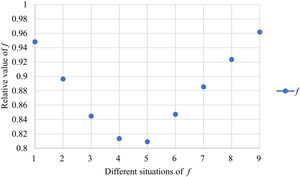
Fig. 2 reveals the tendencies of the objective function f from Situation I to III. Fig. 3 reveals the tendencies of objective function f from Situation IV to VI. Fig. 4 reveals the tendencies of objective function f from Situation VII to IX. In light of Figs. 2-4, the overall tendencies of f from Situation I to IX can be acquired, as displayed in Fig. 5. From the figure, we can see that objective function f decreases first and then increases, reaching the minimum in Situation V.
As shown in Figs. 2-5, we mainly discuss the impact of the different priorities of the bilateral agents on the objective function f=ωχθχ+ωγθγ. Fig. 5 shows a comprehensive comparison. The results show that when the priorities of the bilateral agents differ greatly, the value of the objective function is also greater; however, when the priorities of the bilateral agents gradually tend to be equal, the value of the objective function gradually decreases and tends to be the minimum.
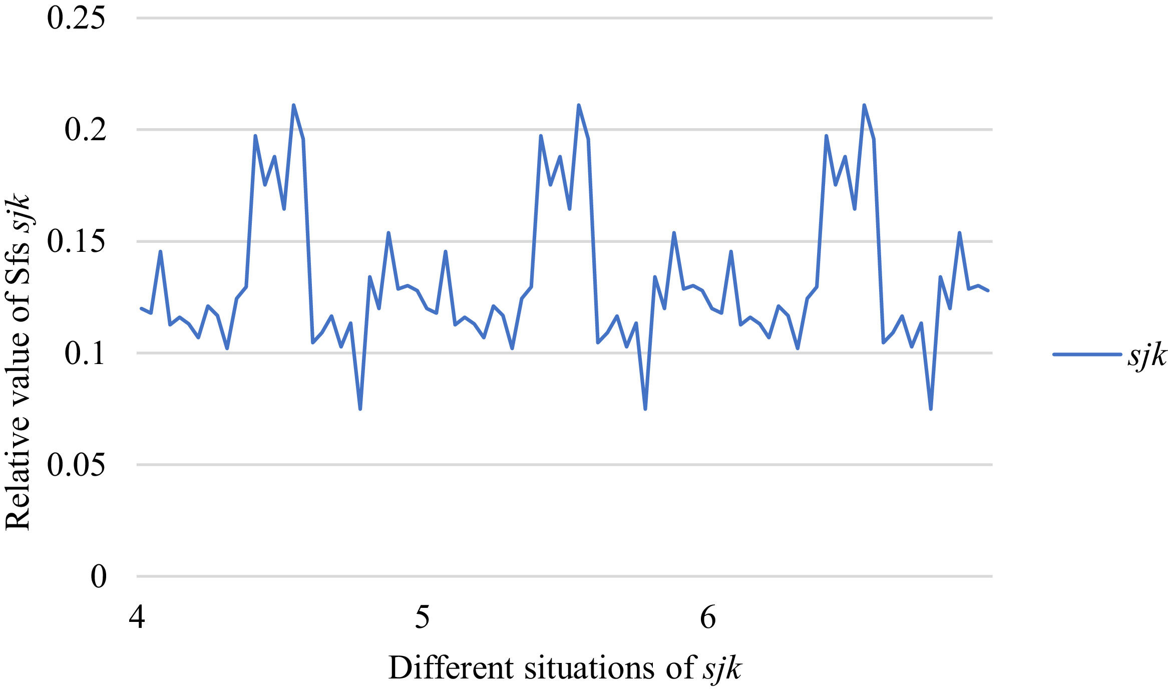
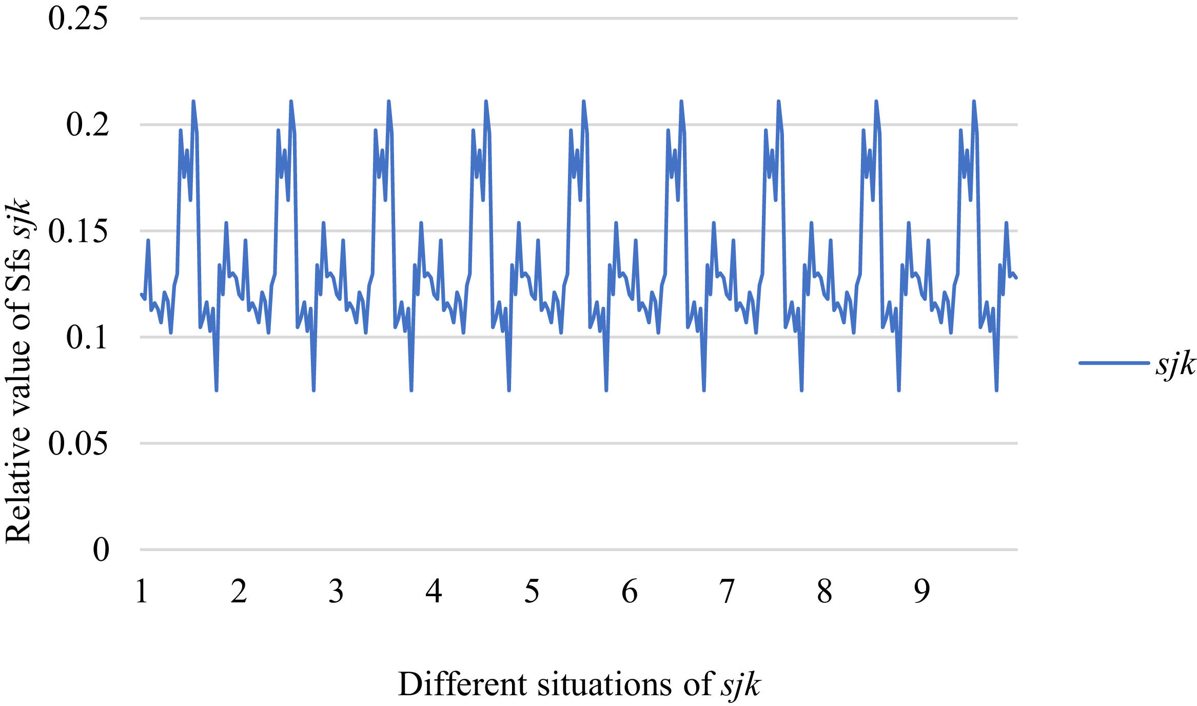
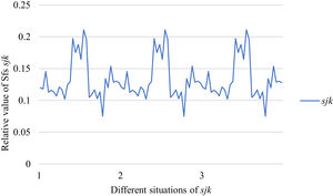
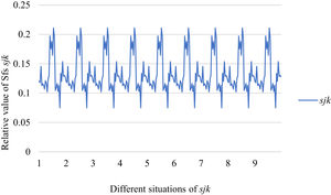
Fig. 6 reveals the tendencies of SFs sF¯jχk from Situation I to III. Fig. 7 reveals the tendencies of SFs sF¯jχk from Situation IV to VI. Fig. 8 reveals the tendencies of SFs sF¯jχk from Situation VII to IX. In light of Figs. 6-8, the overall tendencies of SFssF¯jχk from Situation I to IX can be acquired, as displayed in Fig. 9. From Fig. 9, we can see that SFs sF¯jχk fluctuates periodically from Situation I to IX.
As shown in Figs. 6-9, we mainly discuss the impact of the different priorities of the bilateral agents on SFs sF¯jχk. Fig. 9 shows a more comprehensive comparison. The results show that when the priorities of the bilateral agents are different, there is no significant change in the value of SFs sF¯jχk.
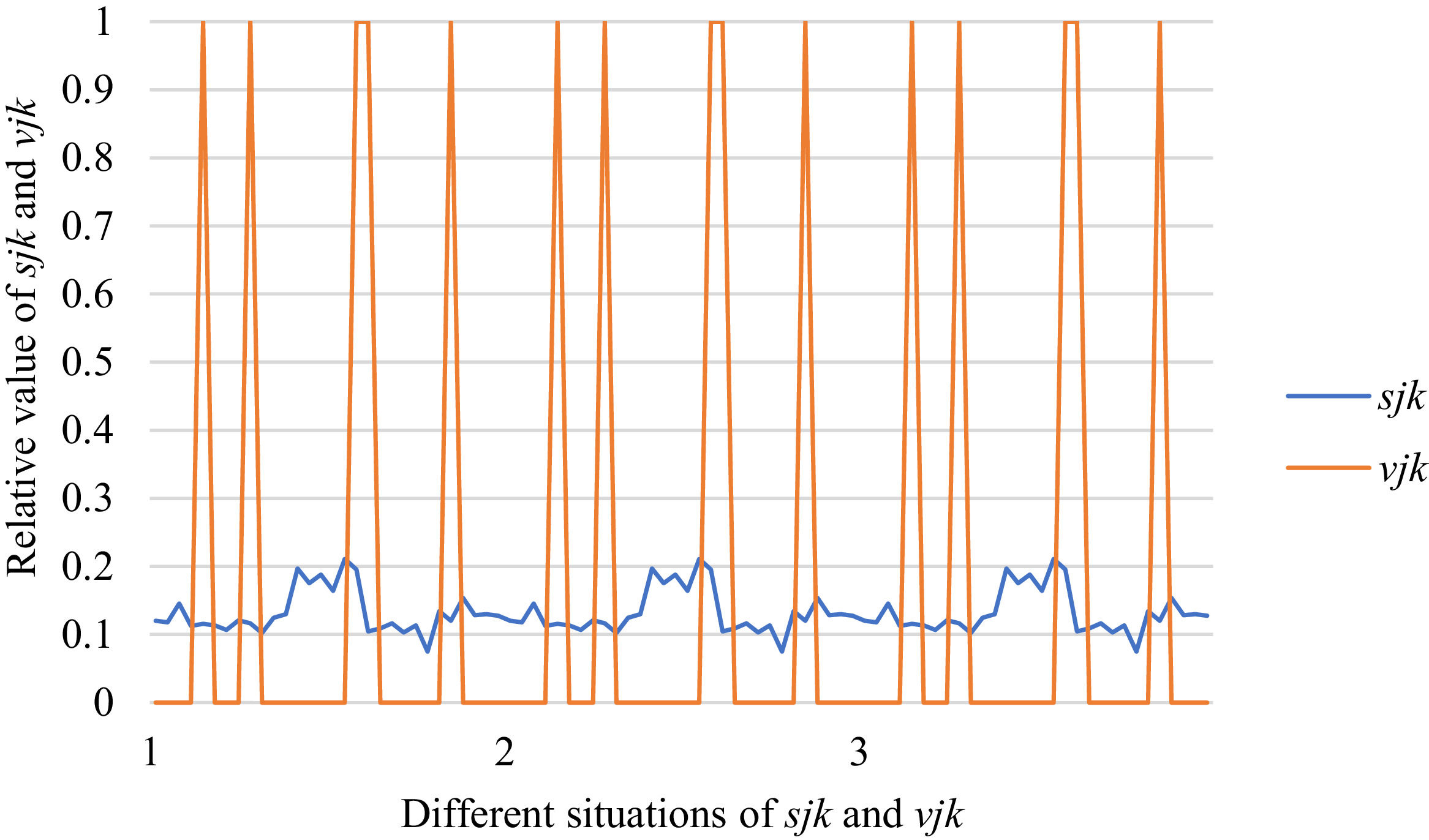
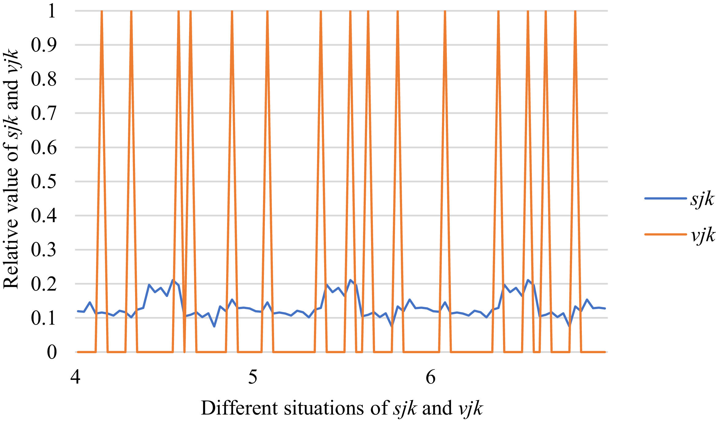
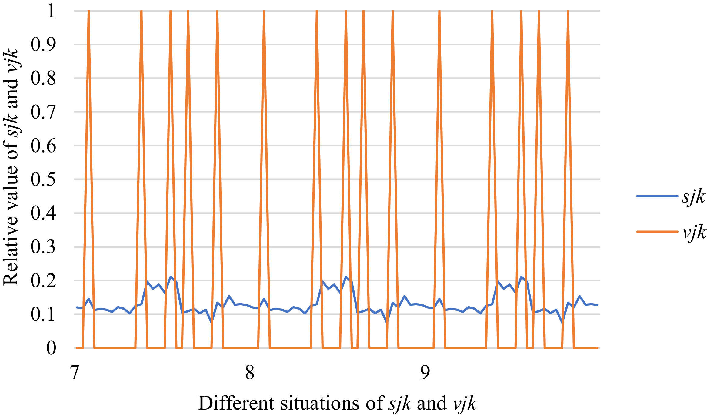
Fig. 10 reveals the tendencies of the relationships among SFs sF¯jχk and the optimal BM matrix V=[vjk*]5×6 from Situation I to III. Fig. 11 reveals the tendencies of the relationships among SFs sF¯jχk and the optimal BM matrix V=[vjk*]5×6 from Situation IV to VI. Fig. 12 reveals the tendencies of the relationships among SFs sF¯jχk and the optimal BM matrix V=[vjk*]5×6 from Situation VII to IX. In light of Figs. 10-12, the overall tendencies of the relationships among SFs sF¯jχk and the optimal BM matrix V=[vjk*]5×6 from Situation I to IX can be acquired, as displayed in Fig. 13. From the figure, we can see that SFs sF¯jχk and the optimal BM matrix V=[vjk*]5×6 are different in some situations.
As shown in Figs. 10-13, we further discuss the influence of the difference priorities on SFs sF¯jχk and the optimal BM matrix V=[vjk*]5×6. Fig. 13 shows a more comprehensive comparison and results. The results show that the priority difference of the bilateral agents has no significant impact on SFs sF¯jχk and the optimal BM matrix V=[vjk*]5×6.
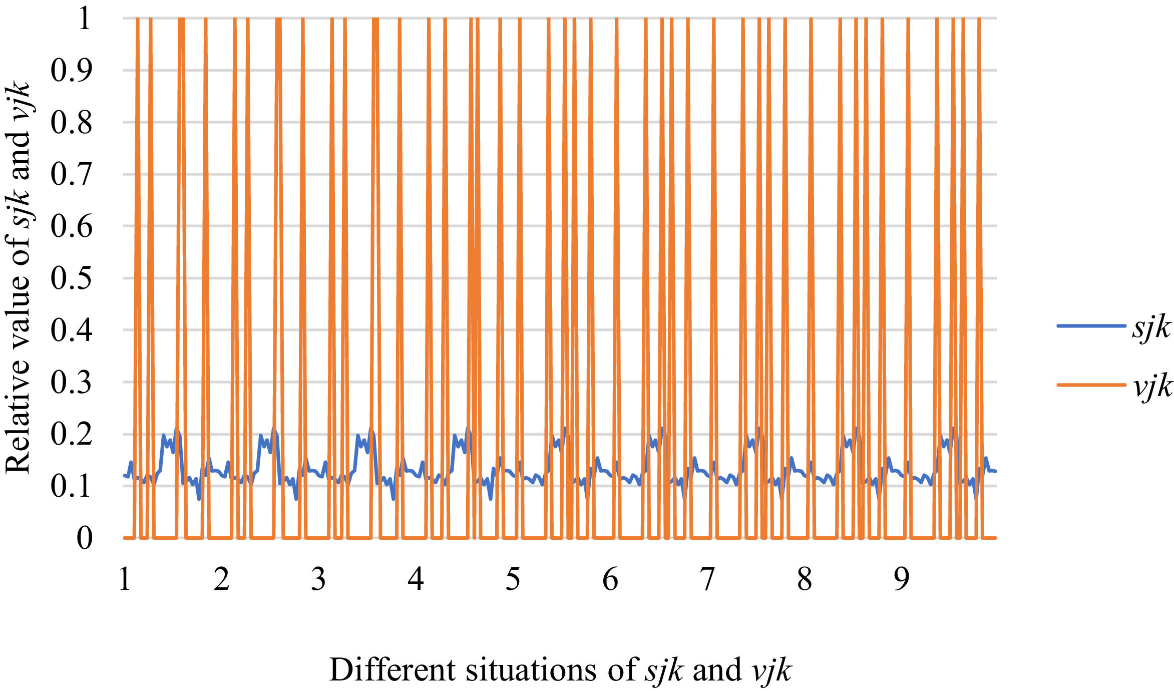
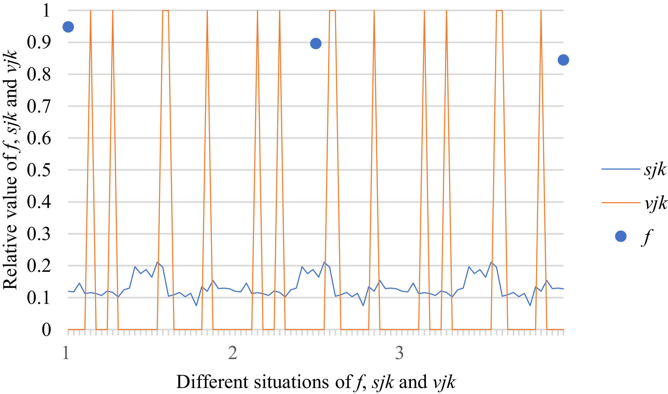
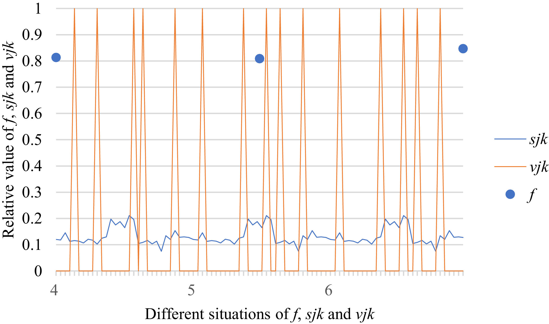
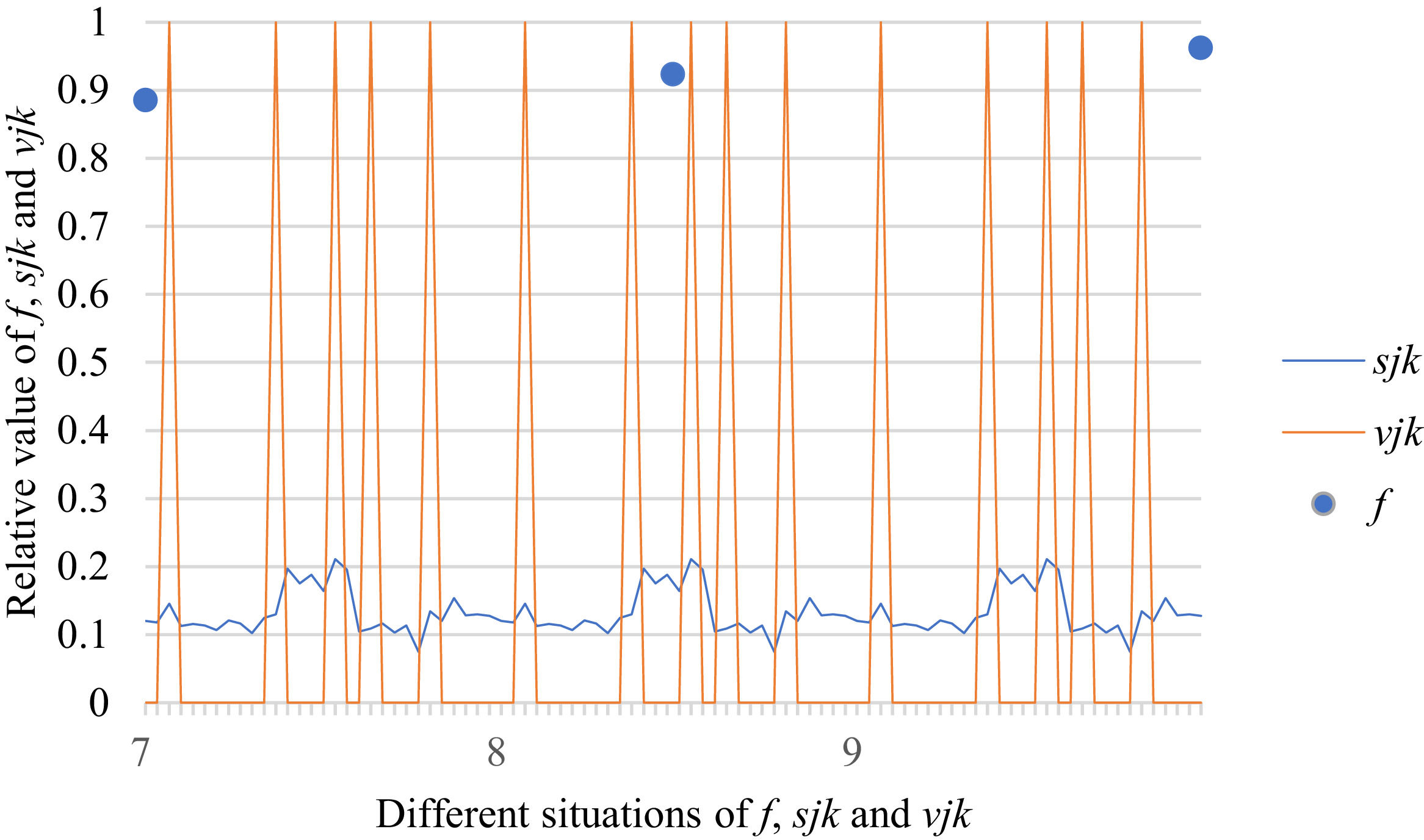
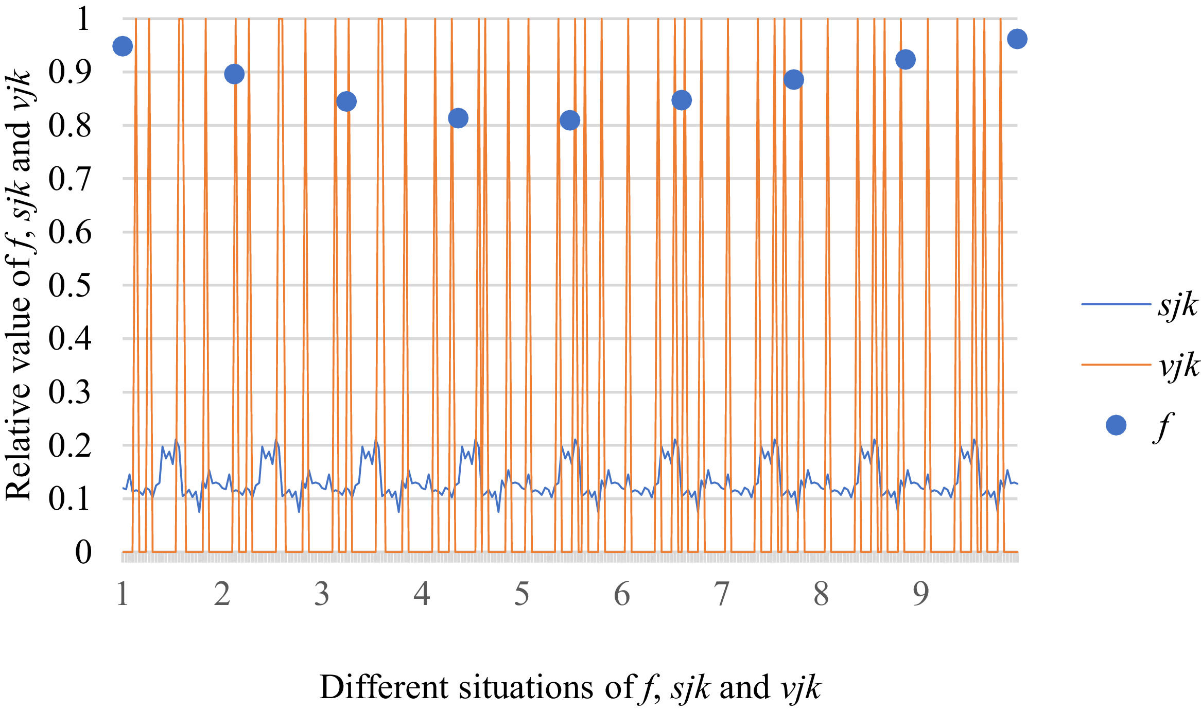
Fig. 14 reveals the tendencies of the relationships among the objective function f, SFs sF¯jχk and optimal BM matrix V=[vjk*]5×6 from Situation I to III. Fig. 15 reveals the tendencies of the relationships among the objective function f, SFs sF¯jχk and optimal BM matrix V=[vjk*]5×6 from Situation IV to VI. Fig. 16 reveals the tendencies of the relationships among the objective function f, SFs sF¯jχk and optimal BM matrix V=[vjk*]5×6 from Situation VII to IX. In light of Figs. 14-16, the overall relationships among the objective function f, SFs sF¯jχk and optimal BM matrix V=[vjk*]5×6 from Situation I to IX can be acquired, as displayed in Fig. 17. From the figure, we can see that the objective function f is different in all situations; meanwhile, SFs sF¯jχk and optimal BM matrix V=[vjk*]5×6 are different in some situations.
As shown in Figs. 14-17, we further discuss the influence of the different priorities of the bilateral agents on the objective functionf, SFs sF¯jχk and optimal BM matrix V=[vjk*]5×6. Fig. 17 shows a more comprehensive comparison and results. The results show that the different priorities of the bilateral agents will have a significant impact on the objective function value f in this experimental analysis but it has no significant impact on SFs sF¯jχk and the optimal BM matrix V=[vjk*]5×6 in this experimental analysis. Considering this experimental analysis, shows that the priority of the agent is only one of the factors affecting the determination of the optimal BM scheme but is not the decisive factor. However, if the same analysis is performed for the other examples, the results may not be exactly the same.
ConclusionsExamining the BM problem of knowledge innovation management under an interval intuitionistic fuzzy set environment, a matching decision-making method is proposed. In the method, the matching willingness of the bilateral agents is obtained by developing a novel algorithm, and a BM model considering IvIFSs and the matching willingness is constructed. The optimal BM scheme is obtained through the model solution. An enterprise knowledge management case study verifies the effectiveness of the presented BM method. The method proposed in this paper is applicable to a variety of intuitionistic fuzzy preference environments considering the matching willingness of the bilateral agents and can also be applied to other decision-making problems in enterprise knowledge innovation management.
Compared with the existing methods, the presented approach exhibits the following salient features: (1) The displayed approach uses the TOPSIS technology to compute the matching willingness directly on the basis of the IvIFS preferences, which can avoid information loss as much as possible. The computational algorithms of matching willingness can be regarded as a generalization of the existing approaches. (2) The displayed approach establishes the BM model using IvIFSs and matching willingness, which can mirror agents’ behaviours that are overlooked in some existing approaches. (3) The displayed approach uses a new optimization algorithm to solve the developed BM model, which is a new approach and supplement to the existing algorithms. (4) The gained BM scheme can reflect agents’ matching willingness, which has been overlooked in many existing approaches.
Future research will mainly focus on the following areas: (1) the BM problem with IvIFSs needs an in-depth study, where the matching willingness of a single agent towards the agents of the other side is not at the same level. (2) Considering that stable matching has an impact on the satisfaction of the bilateral agents and that an unstable BM scheme may reduce the satisfaction of the bilateral agents, we will additionally study the relevant theories and methods for stable matching in the IvIFS environment. (3) This paper mainly focuses on the IvIFS environment; therefore, the calculation algorithm of matching willingness under other intuitionistic fuzzy preferences needs to be further studied.
This work was partly supported by the National Natural Science Foundation of China (Grant No. 71861015), the Humanities and Social Science Foundation of the Ministry of Education of China (Grant No. 18YJA630047), the Distinguished Young Scholar Talent of Jiangxi Province (Grant No. 20192BCBL23008).










![Relationships among SFs sF¯jχk and the optimal BM matrix V=[vjk*]5×6 from Situation I to III. Relationships among SFs sF¯jχk and the optimal BM matrix V=[vjk*]5×6 from Situation I to III.](https://static.elsevier.es/multimedia/2444569X/0000000700000003/v1_202207240530/S2444569X2200049X/v1_202207240530/en/main.assets/thumbnail/gr10.jpeg?xkr=ue/ImdikoIMrsJoerZ+w96p5LBcBpyJTqfwgorxm+Ow=)
![Relationships among SFs sF¯jχk and the optimal BM matrix V=[vjk*]5×6 from Situation IV to VI. Relationships among SFs sF¯jχk and the optimal BM matrix V=[vjk*]5×6 from Situation IV to VI.](https://static.elsevier.es/multimedia/2444569X/0000000700000003/v1_202207240530/S2444569X2200049X/v1_202207240530/en/main.assets/thumbnail/gr11.jpeg?xkr=ue/ImdikoIMrsJoerZ+w96p5LBcBpyJTqfwgorxm+Ow=)
![Relationships among SFs sF¯jχk and the optimal BM matrix V=[vjk*]5×6 from Situation VII to IX. Relationships among SFs sF¯jχk and the optimal BM matrix V=[vjk*]5×6 from Situation VII to IX.](https://static.elsevier.es/multimedia/2444569X/0000000700000003/v1_202207240530/S2444569X2200049X/v1_202207240530/en/main.assets/thumbnail/gr12.jpeg?xkr=ue/ImdikoIMrsJoerZ+w96p5LBcBpyJTqfwgorxm+Ow=)
![Relationships among SFs sF¯jχk and the optimal BM matrix V=[vjk*]5×6 from Situation I to IX. Relationships among SFs sF¯jχk and the optimal BM matrix V=[vjk*]5×6 from Situation I to IX.](https://static.elsevier.es/multimedia/2444569X/0000000700000003/v1_202207240530/S2444569X2200049X/v1_202207240530/en/main.assets/thumbnail/gr13.jpeg?xkr=ue/ImdikoIMrsJoerZ+w96p5LBcBpyJTqfwgorxm+Ow=)
![Relationships among the objective function f, SFs sF¯jχk and optimal BM matrix V=[vjk*]5×6 from Situation I to III. Relationships among the objective function f, SFs sF¯jχk and optimal BM matrix V=[vjk*]5×6 from Situation I to III.](https://static.elsevier.es/multimedia/2444569X/0000000700000003/v1_202207240530/S2444569X2200049X/v1_202207240530/en/main.assets/thumbnail/gr14.jpeg?xkr=ue/ImdikoIMrsJoerZ+w96p5LBcBpyJTqfwgorxm+Ow=)
![Relationships among the objective function f, SFs sF¯jχk and optimal BM matrix V=[vjk*]5×6 from Situation IV to VI. Relationships among the objective function f, SFs sF¯jχk and optimal BM matrix V=[vjk*]5×6 from Situation IV to VI.](https://static.elsevier.es/multimedia/2444569X/0000000700000003/v1_202207240530/S2444569X2200049X/v1_202207240530/en/main.assets/thumbnail/gr15.jpeg?xkr=ue/ImdikoIMrsJoerZ+w96p5LBcBpyJTqfwgorxm+Ow=)
![Relationships among the objective function f, SFs sF¯jχk and optimal BM matrix V=[vjk*]5×6 from Situation VII to IX. Relationships among the objective function f, SFs sF¯jχk and optimal BM matrix V=[vjk*]5×6 from Situation VII to IX.](https://static.elsevier.es/multimedia/2444569X/0000000700000003/v1_202207240530/S2444569X2200049X/v1_202207240530/en/main.assets/thumbnail/gr16.jpeg?xkr=ue/ImdikoIMrsJoerZ+w96p5LBcBpyJTqfwgorxm+Ow=)
![Relationships among the objective function f, SFs sF¯jχk and optimal BM matrix V=[vjk*]5×6 from Situation I to IX. Relationships among the objective function f, SFs sF¯jχk and optimal BM matrix V=[vjk*]5×6 from Situation I to IX.](https://static.elsevier.es/multimedia/2444569X/0000000700000003/v1_202207240530/S2444569X2200049X/v1_202207240530/en/main.assets/thumbnail/gr17.jpeg?xkr=ue/ImdikoIMrsJoerZ+w96p5LBcBpyJTqfwgorxm+Ow=)
