


The agricultural economy plays an irreplaceable and crucial role in ensuring national food security, promoting stable economic growth, and fostering harmonious social development. Agricultural technology innovation (ATI) and rural industrial structure transformation (RIST) are key drivers of agricultural economic growth (AEG). Although previous studies have largely focused on the individual impacts of ATI and RIST on AEG, research on the specific pathways linking these factors is limited. This study utilizes panel data from 30 Chinese provinces from 2009 to 2022 and employs a multilayer structural equation model to systematically examine the relationships among ATI, RIST, and AEG at both national and regional levels. In addition, it provides an in-depth analysis of the internal connections among specific variables. The findings indicate that, at the national level, ATI plays a crucial role in significantly advancing both the transformation and upgrading of rural industrial structures and AEG. However, the direct impact of RIST and upgrading on AEG is not clearly evident. The regional-level analysis reveals that ATI has a significant positive effect on AEG and promotes the optimization of rural industrial structures. In addition, upgrading rural industrial structures significantly enhance AEG. This study’s methodology offers both theoretical and empirical support for promoting agricultural economic development through ATI and RIST upgrading. The findings provide valuable insights for policymakers, enabling them to better align agricultural policies with key innovation directions and structural improvements, ultimately fostering sustainable agricultural development. Furthermore, the conclusions serve as a decision-making reference for agricultural enterprises and practitioners, guiding them to adapt to industrial structural adjustments, leverage technological advancements, and enhance agricultural production efficiency and economic benefits.
In the process of modern agricultural development, as a fundamental industry, agriculture plays a vital role in ensuring economic and social stability in various countries. However, agricultural development is now facing unprecedented challenges. On the one hand, resource shortages have become increasingly prominent, with limited arable land and water resources imposing strict constraints on agricultural production (Calicioglu, 2019). Conversely, consumer demand for agricultural products is becoming more diverse and high-end, requiring not only adequate quantity but also higher standards of quality, safety, and nutrition (Rana, 2017). Against this backdrop, agricultural technology innovation (ATI) and rural industrial structure transformation (RIST) have become key approaches for addressing these challenges. Previous studies have recognized the positive effects of ATI and RIST on agricultural economic growth (AEG). Through theoretical analysis and empirical research, numerous scholars have confirmed that ATI improves agricultural production efficiency and reduces production costs, whereas RIST expands the agricultural industry chain and increases the added value of agriculture. Both provide strong momentum for AEG. However, the existing research has some limitations, leaving room for further exploration. In terms of research methods, most current studies use linear regression models to analyze these issues, lacking a multidimensional and comprehensive analytical framework. As a result, it is difficult to fully describe the indicators that influence ATI, RIST, and AEG, as well as the complex relationships among them. From a research perspective, most studies have focused on the direct relationships among these three factors, with relatively little exploration of the specific pathways through which ATI and RIST affect AEG or the internal mechanisms underlying their interactions.
Given the aforementioned deficiencies, conducting this research using China as an example is well-founded. Although China’s agricultural arable land accounts for only 3 % of the world’s total, its population comprises 18.8 % of the global population. This situation necessitates a shift from merely increasing production volume to emphasizing high-quality production (Liu & Li, 2017). As modern agriculture develops, the division of labor within agriculture has become increasingly refined, and rural areas in China have gradually exhibited distinct characteristics across primary, secondary, and tertiary industries. According to the “Classification and Codes of National Economic Sectors,” these three industries can be classified as follows: the primary industry includes agriculture, forestry, animal husbandry, and fishery in rural areas; the secondary industry refers to rural industries and construction; and the tertiary industry includes rural service industries and other sectors not covered by the first two (Guo et al., 2010). The achievements and challenges that China has faced in ATI and RIST can offer valuable insights for other developing countries. For instance, China’s technological innovation practices in areas such as agricultural mechanization and informatization, as well as its integrated development model across primary, secondary, and tertiary industries in rural areas, can serve as reference examples for other nations. In addition, China’s policy measures and practical experience in addressing the issue of unbalanced regional development can help other countries tackle similar agricultural development challenges. Through this research, promoting China’s agricultural development experience on an international scale will contribute to the shared development of the global agricultural economy.
The marginal contribution of this research is the empirical testing of the relationships among ATI, RIST, and AEG by constructing and analyzing a structural equation model (SEM), thereby revealing the underlying influencing mechanisms. Specifically, this study includes the following aspects: First, it clarifies the direction and degree of influence of different types of ATI on RIST. Second, we explored the mediating role of RIST between ATI and AEG. Third, this study analyzes how regional heterogeneity factors moderate the relationships among ATI, RIST, and AEG. The results of this research contribute to a deeper understanding of the sources and dynamic mechanisms of AEG, serving as a reference for decision-making in developing rural industrial policies, adjusting the rural economic structure, and implementing the rural revitalization strategy. In addition, these findings promote the comprehensive development of the rural economic society.
The rest of this paper is organized as follows. Section 2 systematically reviews the existing literature on the interactions among ATI,RIST, and AEG. This analysis provides a foundational reference for constructing the model and developing hypotheses in this study. Section 3 discusses the mechanisms of action and research hypotheses, where the paper carefully derives the impact of ATI on the upgrading of the agricultural industrial structure, the contribution of such structural upgrading to economic growth, and the influence of ATI on the enhancement of agricultural economic output. Section 4 covers the research design and introduces the data sources and collection methods, the selection of evaluation indicators, and the construction of the multilevel structural equation model (MSEM). Section 5 presents the empirical analysis in which we empirically analyze the impact of ATI and RIST on AEG using the MSEM, discuss the empirical test results, and reveal the pathways through which ATI and RIST affect AEG. Section 6 presents the discussion, which compares the marginal contributions of this study’s results with those of previous research and addresses the remaining limitations of the study. Section 7 presents the conclusions and policy recommendations.
Literature review and hypothesis statementATI is a core driving force behind the development of the agricultural economy. The significance of this approach lies in the improvement of the quality and efficiency of production factors, the enhancement of land productivity, and the promotion of sustainable development. At the labor force level, technological innovation has driven agricultural mechanization and automation, significantly freeing labor and enabling the workforce to engage in higher-value-added work, thus improving labor productivity. In addition, it attracts capital investments into the agricultural sector, therefore optimizing the efficiency of capital allocation (Mugoni, 2023). Furthermore, innovations in ecological agricultural technologies, such as the use of organic fertilizers and biological pest control, have effectively reduced the reliance on chemical inputs, protected the ecological environment, improved the quality and market competitiveness of agricultural products, and promoted the long-term, stable growth of the agricultural economy (Hazell, 2024). However, despite the theoretical recognition of ATI as a key driver of economic growth, farmers face a dilemma between traditional low-risk and innovative high-risk technologies when investing in production technologies. Because of factors such as risk aversion, farmers often exhibit a low rate of technology adoption. As a result, investments in agricultural technology have a limited impact on driving AEG (Wu, 2023).
At the same time, optimizing and upgrading the rural industrial structure is a crucial way to promote rural economic growth. By extending the agricultural industry chain, optimizing the industrial structure fosters the all-around development of agricultural products, from planting and processing to sales, thereby increasing the added value of agriculture (Ji, 2024). A diversified industrial structure enhances the resilience of the rural economy, providing a buffer when agricultural production faces natural disasters or market fluctuations. In addition, it stimulates the growth of nonagricultural industries, such as rural e-commerce and handicrafts, creating new sources of income for rural areas (Cui, 2023). However, the rapid introduction of modern technologies and the swift adjustment of the industrial structure can adversely impact traditional agriculture, worsening the wealth gap and affecting regional economic stability (Tian, 2024).
Some scholars have further suggested that ATI does not directly affect economic growth but exerts its influence indirectly by promoting the optimization of the industrial structure. On the one hand, technological innovation improves the processing technology of agricultural products and their added value, effectively extending the industrial chain and driving the transformation and upgrading of agriculture toward the processing and manufacturing industries (Ji, 2024). Conversely, technological innovation facilitates the integration of agriculture with the secondary and tertiary industries, giving rise to new industrial forms such as agritourism and rural tourism, thereby injecting fresh growth momentum into the rural economy (Hu, 2023). However, when market conditions are severely flawed, such as through poor sales channels, it becomes difficult to realize the economic benefits of technological innovation. Instead of promoting the optimization of the industrial structure to foster rural economic growth, technological innovation may result in a waste of resources (Hazell, 2024).
Existing research has extensively explored the positive effects of ATI on enhancing production efficiency, optimizing resource allocation, and promoting sustainable development. Scholars have also examined how the optimization of the rural industrial structure promotes rural economic growth by extending the industrial chain, developing nonagricultural industries, and strengthening economic resilience. However, several deficiencies remain. First, an in-depth analysis of the specific aspects of ATI and its impact pathways and degrees on AEG is lacking. Mechanisms and contributions of different types of ATI (e.g., mechanization and digital information technology innovation) to promote AEG are still unclear. Second, most studies on the relationship between ATI and RIST have focused on static analysis, with little attention paid to the dynamic interactions between the two. Third, differences in agricultural development conditions and environments across regions may lead to significant variations in the relationships among ATI, RIST, and AEG. However, the regional heterogeneity factors have not been sufficiently addressed in existing studies. The innovations of this study can be mainly reflected in two aspects. First, in terms of research perspective, this study not only focuses on the direct impacts of ATI and RIST on AEG but also explores internal connections and interaction mechanisms, as well as the moderating role of regional heterogeneity. Second, in terms of research methods, the use of the MSEM effectively addresses the complex relationships among multiple variables. Furthermore, by considering factors at both national and regional levels, the accuracy and reliability of the research results can be enhanced.
Mechanism and hypothesis of actionImpact of agricultural scientific and technological innovation on upgrading agricultural industrial structuresTo reflect the role of ATI in upgrading the industrial structure, this study proposes distinguishing between traditional and modern agricultural production functions, as outlined below:


Eq. (1) represents the traditional agricultural production function, which excludes capital input and considers labor (La) as the sole factor of production. This assumption reflects the labor-intensive nature of output in traditional agriculture. Eq. (2) represents the modern agricultural production function, which assumes a constant-returns-to-scale Cobb–Douglas (C-D) form. In this equation, output is influenced by both capital (Kb) and labor (Lb) inputs, indicating that modern agricultural production not only depends on labor but also requires adequate capital support. The symbol A represents total factor productivity, which, in the context of traditional agriculture, primarily reflects production efficiency, whereas, in modern agriculture, it denotes the level of technology. The terms δ, α, and β denote the output elasticities with respect to capital and labor inputs, where 0<δ≤1,α+β=1.
The expression for profit maximization in agricultural production is as follows:


By taking the first derivative of Eqs. (3) and (4), we obtain the relative marginal product values of labor (Wa) with respect to the price level of labor in traditional agriculture and the relative marginal product values of labor (Wb) with respect to the price level of labor in modern agriculture, respectively. This can be expressed as follows:


Considering that most of the agricultural labor force is engaged in basic production activities, such as planting and breeding, the skills and knowledge required within a certain scope exhibit similarities. Although rural education levels have improved in recent years, they have primarily focused on basic agricultural production techniques, leading to a certain degree of homogeneity in agricultural production capabilities (Zhong, 2020). With the acceleration of China’s urbanization process and the advancement of rural economic system reforms, the trend of rural labor being transferred to cities and nonagricultural industries have become increasingly evident. Barriers to the movement of rural labor between urban and rural areas, as well as across different industries, have gradually decreased (Hao, 2016). Therefore, it is assumed that the agricultural labor input is homogeneous and freely mobile, with the wage level for labor equal to the marginal product value of labor employed by firms. In addition, the marginal product value of labor used by each firm is assumed to be equal (Wa=Wb). The expression is as follows:


Taking the derivative of Eq. (8), we obtain ∂(Lb/La)/∂Ab>0. Consequently, it can be inferred that as the level of technology improves, the ratio of Lb/La increases. This indicates that with continuous technological progress, an increasing number of agricultural laborers will shift from traditional to modern agricultural production. Modernized agriculture includes not only the traditional primary sector but also the secondary and tertiary sectors. Moreover, technological advancements have facilitated the movement of rural labor from the primary industry to the secondary and tertiary industries, thereby gradually optimizing and upgrading the agricultural industrial structure. Based on this, the following hypotheses are proposed:
H1a: ATI promotes industrial structure transformation.
H1b: ATI has no impact on industrial structure transformation.
Agricultural economic output consists of various sectors, including the primary, secondary, and tertiary sectors of agriculture. The growth rate of each sector determines the overall size and growth rate of the agricultural economy, which can be expressed as follows:

Taking the derivative with respect to time (t) on both sides, we obtain the following:
where yt and yt′ denote the growth rate and variations in the agricultural economy in different sectors indexed by i, respectively. ρi and ρi′ represent the proportions and changes in each sector, respectively. The growth rate and variations in the rural economy are influenced by both the growth rate of each sector and changes in the industrial structure. Therefore, with the rapid growth of sectoral output and the resulting upgrade of the industrial structure, the growth rate of the rural economy is inevitably enhanced. Therefore, this study proposes the following hypotheses:
H2a: The transformation of the industrial structure can also promote the growth of the agricultural economy.
H2b: Industrial structure transformation fails to promote the growth of the agricultural economy.
To examine the impact of ATI on AEG, this study focuses on a specified production function for modern agricultural production. The production function is expressed as follows:
where Y is output, K is capital, L is labor, and A is total factor productivity. Innovations in ATI include the introduction of new planting, farming, and harvesting techniques that improve labor efficiency. This means that the same amount of labor can produce more agricultural products, which may also include increasing the mechanization of agriculture or enhancing the efficiency of agricultural capital inputs, such as fertilizers, pesticides, and irrigation equipment. An increase in these inputs can lead to higher output per unit of capital.
Through ATI, we expect an increase in factor A. This signifies that, given a certain amount of capital and labor, output will increase even if the quantities of capital and labor remain unchanged. Consequently, ATI shifts the production function upward, resulting in higher levels of output. Therefore, this study proposes the following hypotheses:
H3a: Agricultural technology innovation promotes agricultural economic growth.
H3b: Agricultural technology innovation fails to promote agricultural economic growth.
Drawing from the research of Chang (2018) and other scholars, we collected panel data for 30 provinces in China from 2009 to 2022.1. The dataset includes relevant information on economic growth, agricultural sector innovation, and industrial structural transformation. The data were sourced from the Statistical Yearbook of China, the Rural Statistical Yearbook of China, various provincial statistical yearbooks, and regional agricultural statistical yearbooks in China.
Indicator selection(1) Selection of indicators of agricultural technology innovation (ATI)
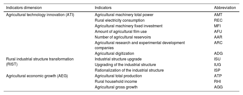
Tisenkopfs et al. (2015) examined improvements in the agricultural technology sector through the input of mechanical equipment and the rate of agricultural mechanization. Their aim was to quantify the development of the agricultural technology sector at the mechanization level using these two indicators. Kim et al. (2020) proposed the hypothesis that the usage of agricultural plastic film and the number of agricultural reservoirs can reflect the level of agricultural modernization. This is because changes in the usage of agricultural plastic film indicate the adoption of new materials in agricultural production, whereas the number of agricultural reservoirs is related to the construction of agricultural irrigation and other infrastructures. The popularization of the Internet and the development of digital technology have brought new opportunities and changes to rural areas (Cheng, 2024). Wang et al. (2019) hypothesized that the average ownership of major durable consumer goods (such as computers and mobile phones) per 100 rural households and the availability of rural Internet broadband access can serve as effective indicators of rural digital infrastructure and digital application carriers. They used the entropy method to calculate the rural digitalization index for each province (autonomous regions and municipalities directly under the Central Government) to measure the level of rural digitalization. Specifically, the total power in agricultural machinery, investment in fixed assets for agricultural machinery, and rural electricity consumption reflect the level of mechanization in agricultural production and the utilization of energy from different perspectives, representing ATI in efficient production. The usage of agricultural plastic film and the number of agricultural reservoirs are closely related to agricultural modernization, reflecting the application of ATI in agricultural infrastructures and production materials. Agricultural research, development, and experimental enterprises are the main drivers of agricultural innovation. Agricultural digitalization, which encompasses rural digital infrastructure and digital applications, is currently the most significant development direction for ATI. Building on the research of previous scholars, this study selects the following indicators to measure ATI: (1) total power of agricultural machinery; (2) rural electricity consumption; (3) fixed investment in agricultural machinery; (4) amount of agricultural plastic film used; (5) number of agricultural reservoirs; (6) agricultural research and experimental development companies; and (7) agricultural digitalization.
(2) Selection of rural industrial structure transformation (RIST)
Wang (2015) used the conversion rate of the industrial structure to illustrate its transformation and upgrading. However, relying solely on the proportion of each industry as a criterion for modifying the industrial structure could lead to an unreasonable distribution of industries. Building on the research of existing scholars, this study considers three aspects of industrial structure modification: conversion rate, improvement, and rationalization of the industrial structure.
First, the conversion rate of the industrial structure is defined by Eq. (12). A higher ratio indicates a higher conversion rate in the industrial structure.

Next, we assess the progress of the industrial structure by examining its upgrading. This can be calculated using the following equation, which offers insights into the development of the service industry.

Third, the rationalization of the industrial structure is a measure of the degree of coordinated development among industries. According to classical economic theory, when the industrial structure reaches equilibrium, all sectors will have the same productivity. Thus, we can obtain Yi∑i=13Yi=Li∑i=13Li, where Yi is the output of industries i and Li represents the employment number of industry i. This type of equilibrium is almost impossible to achieve, and unbalanced development is a normal state. The calculation formula is as follows:
where E represents the rationalization of the industrial structure. The larger the value of E, the greater the deviation from an optimal industrial structure, indicating a more inefficient or unreasonable industrial structure.
(3) Selection of indicators of agricultural economic growth (AEG)
This study builds upon the work of Li et al. (2020) and uses agricultural total output, rural per capita income, and the agricultural output growth rate as indicators to measure AEG. Agricultural total output serves as a crucial metric for assessing the scale and efficiency of the agricultural sector, reflecting changes in agricultural production levels and the overall development of the agricultural economy. Rural per capita income is an important indicator of the economic status and living standards of rural residents because it helps assess the agricultural economy’s impact on rural welfare and its role in reducing rural poverty. The growth rate of agricultural total output indicates the influence of factors such as technological advancements in agricultural production, increased investments, and expanding market demand on the agricultural economy. A higher growth rate indicates rapid development within the agricultural sector, enhancing its competitiveness.
The evaluation indices of ATI, RIST, and AEG used in this study are listed in Table 1.
Evaluation dimensions and agricultural economic growth indices.
The MSEM is an extension of the traditional SEM and multilevel linear model. Goldstein and McDonald (1988) first introduced a general model for multilevel data analysis, which laid the foundation for the development of the MSEM. Later, in 1994, Muthén proposed methods for implementing the MSEM, aiming to address challenges in multilevel data analysis, such as enabling the estimation of random coefficients.
There are complex causal relationships among ATI, RIST, and AEG, encompassing direct, indirect, mediating, and moderating effects. The MSEM can simultaneously estimate these direct and indirect relationships among multiple variables, providing a clearer understanding of these complex interactions. In addition, the agricultural economic system exhibits multilevel structural characteristics at the household, regional, and national levels. Factors at different levels may have varying impacts on AEG. The MSEM allows for the consideration of variables at multiple levels and their interrelationships, thereby enabling more accurate capture of the impact pathways through which ATI and RIST influence AEG across different levels.
This study used data from 30 provinces from 2009 to 2022 to empirically analyze the impact pathways of ATI and RIST on AEG. Given the significant heterogeneity among regions in terms of technological innovation levels, industrial transformation progress, and the foundations of the agricultural economy, the traditional SEM—which assumes that data are independently and identically distributed—is prone to overlooking systematic regional differences. To address this limitation, this study employed the MSEM and established the rationale for stratification using the intraclass correlation coefficient (ICC) test. By fitting a null model (including only the regional random intercept), the proportion of between-group variation (ICC) for the core variables was calculated to assess the necessity of stratification. For ATI, the ICC was 0.27, indicating that 27 % of the variation is attributable to regional differences, reflecting a clear imbalance in technology adoption. For RIST, the ICC was 0.11, indicating moderate regional variation that warrants the control of basic regional effects. For AEG, the ICC was as high as 0.63, meaning that 63 % of the total variation stems from regional differences—far exceeding the medium-effect threshold of 0.10 commonly used in social science research (Kreft & De Leeuw, 1998). These results underscore the substantial impact of regional heterogeneity on core variables. If the hierarchical structure is ignored, the traditional SEM is likely to underestimate the standard errors. Therefore, it is essential to adopt the MSEM to appropriately distinguish between national-level (within-layer) and regional-level (between-layer)2 effects. The regional level is nested within the national level. This hierarchical structure accounts for both the overall data trend and the impact of regional heterogeneity, thus avoiding the bias that arises from treating all data as independently and identically distributed, as is common in traditional analysis methods.
In terms of model selection, given that common factors at the national level exert a consistent impact across all regions, a fixed-effects model effectively captures these systematic and universal influences. Conversely, heterogeneous characteristics at the regional level—including significant differences in unobserved variables such as geographical environment, resource endowment, and local policies—require modeling through random effects to reflect the unique development foundations and trajectories of different provinces. Therefore, this study employed a mixed-effects model that integrates both fixed and random effects, balancing macrolevel commonalities with regional-level heterogeneity to achieve a precise fit for the complex hierarchical data structure.
Furthermore, to test the robustness of the model against the omission of latent variables, a sensitivity analysis was conducted. By excluding typical regions with large agricultural economies that may significantly influence model estimation (such as the major agricultural provinces of Henan and Shandong), the core SEM was re-estimated. The results indicate that fluctuations in key path coefficients did not exceed 8 %, and the significance levels of all core variables remained unchanged. This indicates that the model demonstrates strong robustness to local adjustments in sample composition, and the research conclusions are not significantly affected by extreme values in specific regions or by unobserved latent variables.
(1) Measurement Model
For the three latent variables considered in this study (i.e., the ATI, RIST, and AEG levels), the measurement model outlines the relationships between the observed and latent variables.
The measurement model can be expressed as follows:
At the regional level:

Yijk represents the observed value of the j-th region in the t-th year at the national level on the k-th indicator. The k indicators cover all the observed indicators used to measure the ATI, RIST, and AEG levels.
τk is the overall mean (intercept) of the indicator at the regional level. This reflects the average level of the indicator at the regional level when differences in years and regional heterogeneity are not considered.
λk is the factor loading of indicator k on the latent variable at the regional level. It measures the strength of the association between the observed indicator and the latent variable at the regional level.
ηtjk represents the latent variable at the regional level. Taking the latent variable for the ATI level as an example, this variable represents the actual ATI level in region j in year t. However, this level cannot be directly observed and must be indirectly inferred through multiple observed indicators (e.g., the total power of agricultural machinery in the region and rural electricity consumption).
εtjk is the measurement error of the indicator at the regional level. Because of various random factors present in the measurement process, the observed values cannot fully and accurately reflect the latent variable at the regional level.
At the national level:
γτandγλrepresent the overall average intercept and the overall average regression coefficient, respectively, across all regions and all years.

ςtis the latent variable at the national level, representing the overall level of all regions in the t-th year. For example, it represents the overall level of ATI in the t-th year.
ντ and νλrepresent the regression coefficients of the latent variable at the national level with respect to γτ and γλ, respectively. μτk and μλk denote the error terms.
(2) Structural Model
The equations of the structural model are as follows:
where

αtk is the intercept of indicator variable k at time k,
λBjk is the factor loading of variable k in region j at time k,
βBjt is the observed value of region j at time k,
αk is the total intercept of variable k at the national level,
λWk is the total factor loading of variable k at time t, and
εBjtk and εWtk are the error terms of the first and second layers, respectively.
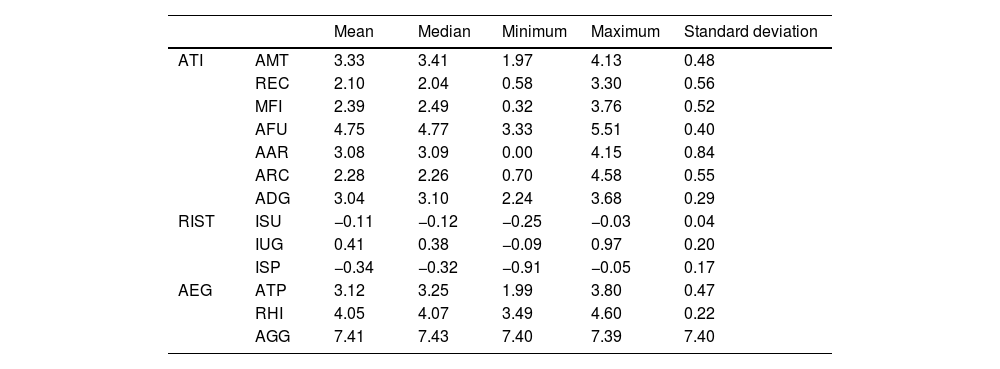
The results the descriptive statistics are presented in Table 2. As shown in Table 2, with respect to ATI, the mean value for the total power of agricultural machinery (AMT) was 3.33, and the median was 3.41, suggesting a relatively concentrated distribution of the data. In terms of rural electricity consumption (REC), the mean was 2.10 with a standard deviation of 0.56, indicating significant variation among the different samples. The statistical values for fixed-asset investment in agricultural machinery (MFI) indicate a relatively stable distribution. For the use of agricultural plastic film (AFU), the minimum value was 3.33, the maximum value was 5.51, and the mean was 4.75, reflecting a relatively stable usage pattern. The number of agricultural reservoirs (AAR) had a minimum value of 0, indicating noticeable differences. The number of agricultural research and experimental development companies (ARC) exhibited minimal fluctuations across the data. Finally, the standard deviation for agricultural digitalization (ADG) was small, indicating low data dispersion.
Descriptive statistics.
In terms of RIST, the mean value for industrial structure upgrading (ISU) was 0.77, indicating a relatively concentrated data distribution. Regarding industrial structure optimization (IUG), the maximum value was 9.32, suggesting the presence of some exceptional individual samples. The statistics for industrial structure rationalization (ISP) indicate that the data were relatively stable.
In terms of AEG, the mean for the total agricultural output value (ATP) was 3.12 with a standard deviation of 0.47, suggesting minimal differences among samples. The data on rural household income (RHI) were relatively concentrated. For total agricultural growth (AGG), the standard deviation were 8.22, with a maximum value of 48.82 and a minimum of −20.88, indicating significant fluctuations and differences.
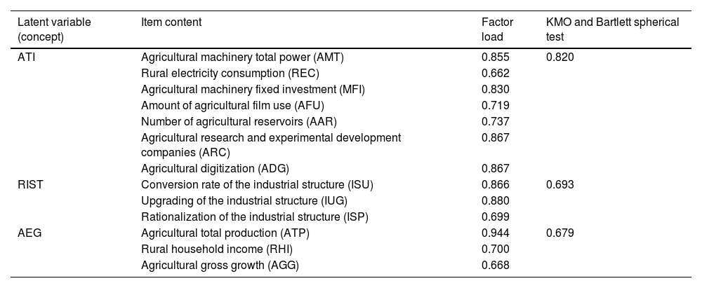
Results of reliability and validity testsIn this study, three exogenous latent variables were constructed: the ATI, RIST, and AEG levels. Table 1 presents specific indicators and their classifications, including total power of agricultural machinery (AMT), REC, fixed-asset investment in agricultural machinery (MFI), usage amount of agricultural plastic film (AFU), number of agricultural reservoirs (AAR), number of agricultural research and development companies (ARC), agricultural digitalization (ADG), industrial structure conversion rate ISU, industrial structure rationalization (ISP), total agricultural output value (ATP), RHI, and total AGG. Before constructing the MSEM, an analysis of the validity of these measurement indicators was conducted to ensure they accurately described the latent variables. This study used SPSS software and conducted factor analysis using the Kaiser–Meyer–Olkin (KMO) measure and Bartlett’s test of sphericity. The reliability and validity results for each variable are presented in Table 3. The results in Table 3 indicate that for AMT, REC, MFI, AFU, AAR, ARC, and ADG, the KMO value was 0.820. A KMO value closer to one indicates stronger partial correlations among variables and greater suitability for factor analysis, confirming that the sampling adequacy is satisfactory. These indicators contain rich information and exhibit a high degree of intercorrelation, effectively reflecting the characteristics of the latent variable of ATI. Similarly, for ISU, IUG, and ISP, the KMO value was 0.693, indicating an acceptable level of sampling adequacy. In addition, for ATP, RHI, and AGG, the KMO value was 0.679, confirming their suitability for factor analysis. Overall, these test results validate the accuracy and reliability of the latent variable descriptions.
Reliability and validity results of each variable.
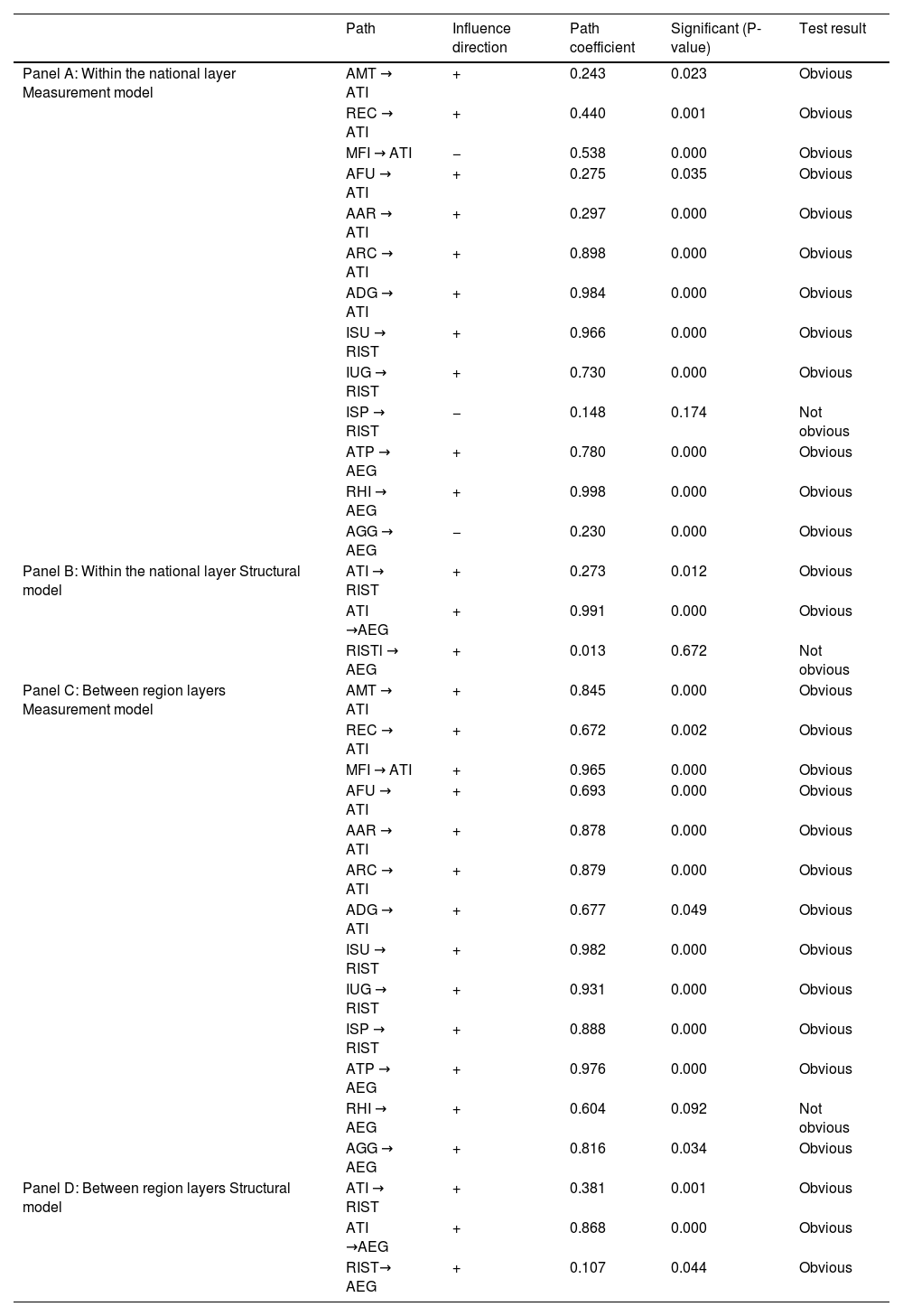
Based on the factor analysis results and the previously outlined theoretical foundations and research hypotheses, this study constructs a two-level framework—“within-layer” (national level) and “between-layer” (regional level)—to analyze the pathways through which ATI, industrial structure improvement, and AEG interact. At the national level, the analysis does not account for regional heterogeneity and uses only the year as the distinguishing index. In contrast, the regional level considers heterogeneity across provinces (cities and districts), incorporating regional indicators to differentiate between various regions. This approach enables a more precise examination of the influence pathways and coefficients of each indicator while accounting for regional heterogeneity. The estimation results of the model are illustrated in Fig. 1, and Table 4 presents the standardized calculation results from the MSEM.

Standardized multilevel structural equation model (MSEM) results.
The results of the standardized MSEM in Table 4 indicate that, although the direct effect of rural scientific and technological innovation (ATI) on economic growth (AEG) is significant, the significance of a single path cannot directly test the overall significance of the indirect effect (a × b) (Hayes & Andrew, 2009). Therefore, a mediating effect test is necessary to uncover the potential transmission mechanism.
This study investigated the mediating transmission mechanism of rural scientific and technological innovation on economic growth by constructing a hierarchical SEM. Common methods for testing mediating effects include the Bootstrap method and Bayesian estimation techniques. However, the Bootstrap method generates new samples through repeated resampling without accounting for the hierarchical structure of the data. This resampling approach, based on the assumption of independent and identically distributed (i.i.d.) data, disrupts intraclass correlations, leading to systematic biases in parameter estimation (Fang et al., 2010). In contrast, hierarchical Bayesian estimation avoids sampling bias for cross-level mediating paths by directly modeling hierarchical random effects (Zitzmann, 2016). Therefore, this study employed a two-level Bayesian estimation approach, decomposing the variance of variables into time-series dynamic effects at the national level (within level) and spatial structural effects at the regional level (between level), and established a dual-path model of “ATI→RIST→AEG.” After 20,000 iterations using the Markov chain Monte Carlo algorithm to obtain the posterior distribution of parameters, the standardized indirect effect values within groups (Within) and between groups (Between) were calculated. The significance was determined based on the 95 % Bayesian credible interval, and if the interval did not contain zero, the existence of the mediating effect was confirmed. The model used a fully standardized solution to present the scale of the cross-level effect while simultaneously controlling for the covariance of the observed indicators to enhance the robustness of the estimation.
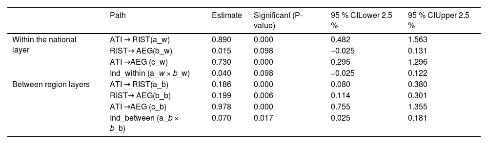
Table 5 presents the test results of the mediating effect under the hierarchical SEM. At the national level (the Within layer), the direct effect of ATI on AEG was significant. However, the P-value of the mediating effect of RIST was 0.098, and the 95 % Bayesian credible interval included zero. Therefore, it failed the test. This indicates that within the framework of national unified policy, limitations exist in the transmission path of industrial structure transformation on economic growth. It may be that policy effects are diluted by regional heterogeneity or that the measurement of indicators fails to fully reflect the dynamic process of the optimization of the internal structure of agriculture.
Test of mediating effect.
At the regional level (the Between layer), both the direct effect of ATI on AEG and the mediating effect of RIST were significant, thus confirming the theoretical mechanism of “ATI → RIST → AEG.” In the context of regional heterogeneity, industrial structure transformation can significantly enhance the economic impact of scientific and technological innovation. This aligns with the real-world scenario where the capital and technological advantages of developed regions drive the upgrading of rural industries.
Robustness testConsidering that the constructed SEM may exhibit model dependence, this study conducted a robustness test by substituting the model estimation method. The default estimation method for a general SEM is the maximum likelihood estimation (MLE), which assumes that the data follow a normal distribution. However, economic data indicators often do not fully conform to this assumption. Therefore, we replaced MLE with the weighted least squares mean method (WLS-M) for estimation and re-estimated the model accordingly. Compared with the strict assumption of multivariate normality in MLE, WLS-M adjusts the covariance matrix of observed variables through weighting and incorporates a mean-corrected chi-square test. This approach helps reduce the estimation bias arising from deviations of the data distribution from normality, thereby enhancing model robustness.
Overall, the robustness test results are highly consistent with the original empirical test results in terms of the direction of the relationships among core variables and the significance of key paths. Only slight differences were observed in some path coefficients and significance levels, and no contradictory conclusions emerged, indicating that the research conclusions possess strong reliability. Regarding the significance levels and path coefficients, at the national level, the ISP→RIST path had a P-value of 0.174 and was not significant under MLE, whereas it was significant under WLS-M in the robustness test. This is because WLS-M corrects the underestimated significance of this path, which is caused by data skewness via weighting. Some coefficients were slightly higher or lower under WLS-M than under MLE. For example, at the national level, the coefficient of ATI→RIST increased from 0.273 to 0.744, and at the regional level, the coefficient of AMT→ATI decreased from 0.845 to 0.618. However, both remained significantly in the same direction. These differences stem from the different treatments of the data distribution characteristics by the two methods: MLE estimates based on the “mean effect” under the normal distribution assumption, whereas WLS-M accounts for the “heteroscedasticity effect” of variables under non-normal distributions through weighting. The changes in the coefficients essentially represent a more accurate depiction of the true relationships within the data, rather than contradictions in the conclusions. Because of space constraints, the full robustness test report and goodness-of-fit evaluation are provided in Appendix 1.
Analysis of the measurement modelThis study’s measurement model encompasses the ATI levels, industrial structure transformation, and AEG, as well as the impact relationships among various measurement indicators. During the research process, without considering regional heterogeneity, the data analysis results at the national level are presented in Table 4 panel A. In the regional analysis that considers local characteristics, the results are shown in Table 4 panel C. The specific analysis results are as follows.
(1) Agricultural technology innovation level
Disregarding regional heterogeneity and based on national-level data analysis, the results indicate that agricultural machinery total power (AMT), REC, agricultural machinery fixed investment (MFI), agricultural film use (AFU), the number of agricultural reservoirs (AAR), agricultural research and experimental development companies (ARC), and agricultural digitization (ADG) all had significant impacts on ATI, with path coefficients generally exceeding 0.5. However, the path coefficient for agricultural MFI exhibited a negative correlation. This suggests that regions with more advanced technology and relatively saturated agricultural equipment tend to invest less in agricultural machinery, whereas regions with less advanced technology invest more. In technologically advanced regions where equipment saturation has been reached, further investments yield lower marginal returns, reducing incentive for additional investments. In contrast, less developed regions with equipment shortages benefit more from increased investment, as it rapidly enhances equipment levels and fosters technological innovation catch-up. Therefore, at the national level, higher machinery investment does not necessarily indicate a higher level of agricultural technology. The regional analysis further revealed that after accounting for local characteristics, the aforementioned variables continued to have a significant positive effect on ATI, with all path coefficients exceeding 0.5. Among these, agricultural machinery fixed investment exerted the strongest impact, with a path coefficient of 0.965. This indicates that for every one-unit increase in fixed-asset investment in agricultural machinery, the level of ATI increased by 0.965. This suggests that within regions, after considering local heterogeneity, increasing investment in agricultural machinery strongly enhances regional ATI, likely due to economies of scale. Greater investment improves agricultural production conditions and accelerates the transformation of technological advancements. In contrast, REC had the lowest path coefficient (0.672) among all indicators. This implies that a one-unit increase in REC increased the level of ATI by only 0.672, which is the smallest effect among the considered factors. The likely reason is that rural electricity is already widely available within regions, meaning that its marginal contribution to technological innovation is lower than other determinants.
(2) Rural industrial structure transformation level
In this study, three indices were used to quantify the transformation and upgrading of the rural industrial structure: the conversion rate of the industrial structure (ISU), the upgrading of the industrial structure (IUG), and the rationalization of the industrial structure (ISP). Based on national-level data analysis, excluding regional variability, the results indicate that the transformation and upgrading of RIST are primarily driven by the ISU and IUG indices, whereas the ISP index does not have a statistically significant impact on this process. Specifically, the path coefficient of ISU on RIST was 0.966, indicating a strong positive effect. This suggests that resources rapidly flow into more efficient industrial sectors, accelerating industrial transformation. For example, labor shifts from traditional agriculture to high-value-added agricultural or nonagricultural industries, thereby driving structural change. Meanwhile, the IUG index had a path coefficient of 0.730, highlighting its significant role in upgrading the agricultural industry structure. The insignificance of ISP may be due to its gradual and long-term nature at the national level, which renders its short-term impact on structural transformation less pronounced.
However, upon shifting to the regional-level analysis and considering various regional factors, it became evident that all three indices—ISU, IUG, and ISP—exerted significant positive effects on RIST, with path coefficients all exceeding 0.8. This underscores that at the regional layer, these indices have a more comprehensive and profound impact on the transformation and upgrading of the industrial structure. Notably, the ISU index had a path coefficient as high as 0.982, reflecting its strong ability to optimize the allocation of agricultural resources across China’s different regions. This allows rapid adaptation to changes in market demand and adjustments to industrial structures. ISP becomes significant at the regional level because industrial connections within the region are closer, enabling rational adjustments to enhance overall synergy and promote the transformation and upgrading of the industrial structure.
(3) Agricultural economic growth level
In assessing agricultural economic development levels, the total output values of the primary industry and rural per capita income were observed to significantly influence agricultural economic development, with path coefficients of 0.780 and 0.998, respectively. This indicates that as the output value of the primary sector and farmers’ income increase, the overall level of agricultural economic development correspondingly improves. However, the relationship between the growth rate of the primary industry and agricultural economic development exhibited an inverse correlation, with a path coefficient of −0.230. This result reveals an intriguing phenomenon: regions with higher growth rates may exhibit relatively lower levels of agricultural economic development, whereas those with lower growth rates might demonstrate better economic development. This could reflect a “catch-up effect,” where economically less developed areas experience faster growth than more advanced regions.
Moreover, when regional heterogeneity factors were incorporated into the analysis, we found that the total output value of the primary industry and its growth rate still significantly impacted AEG, with path coefficients of 0.976 and 0.816, respectively. This suggests that at the regional level, both an increase in the output value of the primary industry and an acceleration in its growth rate strongly promote regional agricultural economic development. Notably, the positive impact of the primary industry’s growth rate contrasts sharply with the negative relationship observed at the national level, indicating that at a more granular regional scale, a higher growth rate indeed drives agricultural economic development. However, when regional disparities are considered, the influence of rural per capita income diminishes and is no longer significant for agricultural economic development. This suggests that income growth among farmers does not necessarily contribute to agricultural economic development to the same extent across all regions.
Analysis of the structural modelThe SEM analysis results at the national level are presented in Table 4 panel B. The results show that ATI is a key driver of RIST and significantly promotes AEG, with the path coefficient for AEG reaching as high as 0.991. This underscores the pivotal role of ATI in accelerating the growth of the agricultural economy. However, the direct impact of industrial structure transformation on AEG was found to lack statistical significance. This may be due to the fact that industrial structure adjustment at the national level is a long-term process. The effects of such adjustments on economic growth are subject to lag, making it challenging to demonstrate a direct and significant relationship in the short term.
Upon closer examination of the regional structural model (panel D in Table 4), it becomes evident that ATIs play a significant role in promoting the transformation of the industrial structure and economic growth across diverse regions. In addition, the transformation of the industrial structure within these regions has substantially facilitated the expansion of the agricultural economy. Among the various factors influencing AEG, ATI exhibited the highest path coefficient at 0.868, highlighting its substantial driving force. Although the impact of RIST on AEG was relatively small (path coefficient of 0.107), this value remained statistically significant. This suggests that, despite its limited direct impact, RIST continues to be an influential factor in shaping the AEG trajectories. The transformation of the regional industrial structure has optimized resource allocation to some extent and improved the synergy efficiency of industries within the region. For example, the integrated development of agriculture and related service industries within the region, despite its promoting effect being weaker than the direct impact of technological innovation, still plays a non-negligible role in the growth trajectory of the regional agricultural economy. This factor is one of the broader factors contributing to regional economic development and, with other factors, shapes the development path of the regional agricultural economy.
Adequacy assessment of the modelThe standardized MSEM was evaluated by assessing several key indicators to determine its adequacy. The evaluation results are presented in Table 6.
The chi-square to degrees-of-freedom ratio is calculated by dividing the chi-square value (χ2) by the degrees of freedom (df). The chi-square value measures the divergence between the observed and model-predicted data, whereas the degrees of freedom reflect the number of parameters that can vary freely within the model. Statistically, the ideal range for the chi-square to degrees-of-freedom ratio is between 0 and 5. A smaller ratio indicates a better-fitting model. The comparative fit index (CFI) assesses a model’s quality by comparing the fit of the target model with that of an independent model (a model assuming no correlations among all variables). The calculation relies on the difference in chi-square values between the nested models. The CFI ranges from 0 to 1, with values closer to one indicating a better fit. Typically, a CFI greater than 0.9 is considered a good fit. As shown in Table 6, the CFI value was 0.922, approaching 1, which suggests that the standardized MSEM is a significant improvement over the independent model and effectively explains the intricate relationships among variables, indicating a high degree of congruence between the assumed model structure and the actual data.
The Tucker–Lewis index (TLI), also known as the non-normed fit index, is another indicator used to evaluate model fit. Considering the model’s complexity, the TLI measures the relative fit of the target model compared with the independent model. The TLI ranges from 0 to 1, with values closer to one indicating a better fit. Typically, when the TLI exceeds 0.9, the model fits well. As shown in Table 6, the TLI value was 0.901, indicating a good fit considering the model’s complexity. This suggests that the model effectively captures the underlying structural relationships in the data and represents a significant improvement over the independent model.
The standardized root mean square residual (SRMR) is a crucial indicator for measuring the model’s goodness of fit. This reflects the standardization of the model residuals (the difference between observed and predicted values) and represents the average error magnitude when fitting the model to the data. Statistically, a smaller SRMR value indicates a better model fit. Generally, an SRMR value below 0.08 is considered satisfactory. As shown in Table 6, the SRMR value was 0.068, which is <0.08, indicating that the model fits the data relatively well with a small average error.
Table 7 presents the composite reliability and average variance extraction of the standardized MSEM. As shown in the table, at the Within layer (national level), the composite reliability (CR) of ATI was 0.75, and the average variance extracted (AVE) was 0.35, below the 0.50 threshold. This indicates insufficient convergent validity for the latent variable. This shortfall can be attributed to the multifaceted nature of ATI at the macro scale, which encompasses dimensions such as R&D investment, technology promotion, and facility equipment. Observation indicators across these dimensions may exhibit response biases due to exogenous factors, including economic cycle fluctuations, regional natural condition disparities, and varying policy implementation intensities. For example, increases in R&D investment may not directly translate into technological transformation efficiency, and uneven regional distribution of facility equipment weakens the coherence among indicators, thereby lowering the AVE value. For RIST, the CR was 0.69, and the AVE was 0.50, indicating weak correlation among the indicators, although it still accounted for 50 % of the variance. For AEG, the CR was 0.75, and the AVE was 0.55, both of which met the standard thresholds. At the Between layer (regional level), the CR values for ATI, RIST, and AEG were 0.93, 0.95, and 0.85, respectively, all significantly higher than 0.7. The AVEs of these variables were 0.65, 0.87, and 0.66, respectively, all exceeding the threshold of 0.5. These results indicate that the measurement model at the regional level has strong reliability and validity. Although some indicators of ATI and RIST at the Within layer did not fully meet the standards, the high CR and AVE values at the Between layer suggested that the measurements at the regional level were stable and reliable. Furthermore, AEG demonstrated strong performance at both layers, highlighting the consistency of the measurement of the core variable.
DiscussionThe findings reveal the relationships among ATI, AEG, and industrial structure transformation at both regional and national levels. The results indicate that the total input of agricultural machinery is the most critical factor influencing ATI. In addition, the analysis at the regional level shows that the speed of industrial structure transformation, upgrading, and rationalization significantly contributes to the improvement of the industrial structure. Moreover, this study concludes that the progress of ATI plays a crucial role in promoting industrial structure transformation and has a substantial impact on AEG. These results support the findings of Hazell (2024), Ji (2024), and others. However, this study also revealed the indirect impact of RIST on AEG. At the national level, RIST does not exhibit a significant impact on AEG. Meanwhile, the rationalization of the industrial structure has no significant impact on the level of RIST. At the regional level, rural per capita income does not significantly impact AEG. These nonsignificant results may stem from the following reasons:
- (1)
At the national level, the impact of industrial structure rationalization on the level of RIST is not significant. Industrial structure rationalization reflects the degree of coordination among regional industries. Given China’s vast territory, significant differences exist in development characteristics and economic levels across regions, resulting in notable inter-regional industrial gaps. Therefore, when evaluating industrial structure rationalization on a national scale, it is difficult to fully account for regional differences (Yuan, 2020). This suggests that, at the national level, industrial structure rationalization does not effectively reflect the optimization of the industrial structure.
- (2)
At the national level, the impact of industrial structure transformation on AEG is not statistically significant. The reasons for this can be summarized in three aspects. First, regional heterogeneity and a time lag exist in policy transmission. Wei et al. (2023) demonstrated by tracking the decay curve of policy shocks using a PVAR model that the half-life of policy effects in eastern regions was 2.3 years, compared with 4.1 years in western regions, indicating significant temporal variation in policy implementation effectiveness across different regions. Second, there are limitations to the construction of indicators. The industrial structure transformation index (RIST) used in this study may not fully capture internal structural changes within the agricultural sector. For instance, many commonly used indicators emphasize the share of nonagricultural industries (e.g., the employment or output-value ratios of the secondary and tertiary sectors). However, contributions from agricultural modernization—such as the application of science and technology and the extension of the agricultural value chain—may be underestimated. Furthermore, in the data aggregation process, high transformation rates in developed regions may overshadow the relatively weaker impacts observed at the national average level (Barrett et al., 2019). Third, there exists a paradox of “deagriculturalization” in the economic structure. In economically underdeveloped regions, deagriculturalization does not merely involve reducing the share of agriculture; rather, it entails extending agricultural value chains, integrating resources to build agricultural industry clusters, and actively developing new forms of rural industries, such as agritourism, to promote the rationalization of the industrial structure (Xu et al., 2024). This transformation path centers on agriculture and enhances its overall benefits through diversified expansion. In contrast, economically developed regions, which leverage advantages in technology, capital, and talent, focus their structural optimization on high-end manufacturing and service sectors. By advancing manufacturing toward more sophisticated, green, and technology-intensive directions and by actively cultivating both producer and consumer service industries, these regions pursue industrial upgrading. In this process, industrial structure optimization is primarily reflected in the rapid growth of nonagricultural industries, rather than in substantial improvements in agricultural productivity (Zhang et al., 2022). Therefore, because of significant differences in the driving mechanisms and development trajectories of industrial structure transformation across regions, the relationship between industrial structure indicators and AEG exhibits marked regional heterogeneity, making it difficult to generalize these dynamics within a unified analytical framework.
Industrial structure transformation at the national level often coincides with a decline in the proportion of agricultural output value. For instance, in developed regions, such as Beijing and Shanghai, the share of agricultural GDP has dropped below 1 %. The optimization of their industrial structure is primarily reflected in the growth of nonagricultural industries rather than in improvements in agricultural efficiency. This “deagriculturalization” trend may weaken the correlation between macrolevel industrial structure indicators and AEG (Zhang et al., 2022). (3) At the regional level, no significant impact of rural per capita income on AEG is observed. It should be noted that rural per capita income includes not only the direct economic benefits that farmers obtain from agricultural development but also nonagricultural income earned through participation in other economic activities (Huang et al., 2024). Research at the national level shows that the growth of rural per capita income generally reflects the overall trend of agricultural economic development, meaning that, from a broader perspective, agricultural economic development is a key determinant of rural residents’ income. The growth of rural residents’ income effectively reflects the development of the agricultural economy.
At the regional level, factors influencing changes in rural per capita income are more complex. In regions with relatively high economic and technological development, rural per capita income is generally higher than the national average. In these cases, fluctuations in rural residents’ income may be more influenced by the overall development of the region rather than solely by AEG. As a result, in some regions, rural per capita income may not fully reflect the growth of the agricultural economy, and its correlation with AEG may lack statistical significance.
This study conducted an in-depth exploration of areas such as ATI, RIST, and AEG, yielding valuable insights. However, there are some limitations. First, the research hypotheses are grounded in the context of China’s agricultural development, which may limit the generalizability of the findings. Cultural, economic, and political factors differ significantly across regions. For example, in economically developed areas, well-established infrastructure and financial support can accelerate the effect of ATI on RIST (Wang, 2015). In contrast, regions with more conservative cultural traditions may face greater resistance to new technologies, thus affecting the applicability of the conclusions. Nevertheless, the exploration of agricultural development in the Chinese context offers important insights for global agricultural research, particularly in pioneering studies on agricultural modernization with Chinese characteristics. Second, the model used in this study has limitations in capturing the impacts of broader economic and policy factors. Government policies, such as subsidies, trade regulations, and market fluctuations, play a crucial role in agricultural development but are not fully addressed in this model. For instance, the European Union’s agricultural subsidy policies have significantly promoted ATI (Garrone, 2019). This study does not explore the unique role of such policies in China or their complex relationships with RIST and AEG. Nevertheless, the model offers valuable insights into the direct relationship between ATI and RIST, thus providing a foundation for future research. Finally, existing studies primarily rely on traditional indicators, such as the share of nonagricultural industries, to measure RIST, which may overlook the critical roles of the specialized division of labor and technological penetration within the agricultural sector. For example, the agricultural value chain extension index can more accurately capture the value-added process of agriculture expanding from production to processing, distribution, and service stages (Kalimuthu et al., 2024), whereas the contribution rate of agricultural science and technology directly reflects the impact of technological innovation on agricultural production efficiency (Musajan et al., 2024). However, the absence of such granular, multidimensional indicators in the current statistical system results in structural biases in characterizing ATI and RIST. This lack of detailed indicators also partially explains the lower AVE at the national level because the indicators fail to fully capture the complex internal dynamics of agricultural modernization and technological integration.
Future research could be enhanced in the following ways. First, the research scope could be broadened by incorporating data from a wider variety of regions. This would involve conducting in-depth analyses of how cultural, economic, and political factors impact ATI, leading to the development of a more universal theoretical framework. Second, the model could be refined by incorporating additional economic and policy variables, such as government subsidies, trade policies, and market fluctuations. This would allow for a more accurate simulation of the impact mechanisms of ATI on RIST and AEG in real-world settings. Third, to further refine the selection of indicators, research should strengthen microlevel data collection by obtaining detailed primary information through in-depth surveys of rural households and other methodologies. Incorporating specific metrics such as the “agricultural value chain extension index,” “contribution rate of agricultural science and technology,” “diffusion rate of agricultural technology,” and “number of patents” would enable a more precise assessment of the actual effects of ATI across different hierarchical levels. This approach would provide stronger theoretical support for the formulation of agricultural policies and the advancement of sustainable agricultural development.
Conclusions and policy recommendationsThis study analyzed panel data from 30 provinces in China between 2009 and 2022 using an MSEM to explore the relationships among ATI, AEG, and RIST. The study revealed the following key conclusions. At the national level, ATI plays a crucial role in driving industrial structure transformation and significantly promotes AEG. However, the direct impact of industrial structure transformation on AEG is not significant, likely because of the long-term lag in industrial structure adjustment. At the regional level, ATI strongly facilitates both industrial structure transformation and economic growth. In addition, industrial structure transformation contributes to the expansion of the agricultural economy. Among the factors considered, ATI has the most significant impact on AEG. Although the direct effect of industrial structure transformation on AEG is relatively small, it remains a vital factor, promoting regional agricultural economic development by optimizing resource allocation and improving industrial synergy.
Based on the above conclusions, this study proposes the following policy recommendations:
- 1
Enhance investment and promotion of ATI. The government should increase financial support for ATI by establishing dedicated funding programs and supporting universities and research institutions in agricultural R&D. In addition, agricultural technology promotion and service systems should be developed to accelerate the transformation of scientific research into practical applications. This will ensure the rapid integration of advanced agricultural technologies into production, further strengthening their role in driving AEG.
- 2
Optimize industrial structure adjustment mechanisms. Given the limited direct impact of industrial structure transformation on AEG at the national level, likely due to long-term adjustment lags, a dynamic monitoring and adjustment mechanism should be established. Industrial structure adjustments should be guided by market demands and the evolving agricultural landscape to ensure more efficient resource allocation and shorter adjustment cycles. Special attention should be given to strengthening industries related to agriculture, fostering integrated development across sectors, and enhancing the direct contribution of industrial transformation to AEG.
- 3
Strengthen regional collaboration in ATI and industrial transformation. Regional cooperation in ATI should be enhanced by local resources and industry advantages. Establishing a regional ATI alliance can facilitate the sharing of technological resources and research achievements, thus enabling joint efforts to address key agricultural development challenges. In addition, industrial collaboration among regions should be reinforced to avoid redundant competition, leverage complementary strengths, and collectively promote regional AEG.
Chenggang Li: Writing – original draft, Supervision, Methodology, Funding acquisition, Conceptualization. Cong Luo: Writing – review & editing, Writing – original draft, Methodology. Hongye Jia: Writing – review & editing, Writing – original draft, Methodology, Formal analysis, Data curation, Conceptualization. Mu Yue: Writing – review & editing, Visualization, Supervision, Methodology. Liang Wu: Supervision, Investigation, Funding acquisition, Formal analysis.
This study is supported by Guizhou Province Major Science and Technology Achievement Transformation Project (QKHCG[2024]ZD016), Guizhou Provincial Education Department Natural Science Research Project (Qian Jiao Ji [2023] No.033), 2024 Quality Development Project of Administration for Market Regulation of Guizhou Province (No.: Guizhou Quality Development Project [2024] No. 6).
Robustness test results
Robustness test and fit evaluation
Since data for most regions are only available up to 2022 and considering the incomplete and severely limited data coverage in China’s Tibet Autonomous Region, this study focuses on analyzing data from 30 regions, excluding Tibet. Data source: https://data.cnki.net/homeSince data for most regions are only available up to 2022 and considering the incomplete and severely limited data coverage in China’s Tibet Autonomous Region, this study focuses on analyzing data from 30 regions, excluding Tibet. Data source: https://data.cnki.net/home Since data for most regions are only available up to 2022 and considering the incomplete and severely limited data coverage in China’s Tibet Autonomous Region, this study focuses on analyzing data from 30 regions, excluding Tibet. Data source: https://data.cnki.net/home
The hierarchical variable in this study is the regional variable. Specifically, at the national level (the within layer), dynamic effects are analyzed annually. At the regional level (the between layer), the influence of macropolicy time trends and regional economic differences is separated by identifying different regions.
articles