In this paper we present and confront the expected outcome of an increase in risk on the regional or sectoral allocation of labor force and employment. The basic frameworks are the benchmark dualistic scenarios. A single-input analysis of a homogeneous product economy is provided. Uncertainty is modeled as localized Bernoulli random experiments, additively affecting either labor demand or labor productivity, unilaterally, or in a perfectly (positive and negative) correlated fashion in both regions providing a stage from which conclusions on the expected consequences of random shocks (or of changes in workers’ heterogeneity) to the economy can be drawn. A (deterministic) differentiated natural appeal of —an intrinsic imbalance between, a compensating income differential required by affiliates of one sector— the two regions is allowed to interact with equilibrium formation.
We report the main effects on equilibrium local expected wages, supply, employment and aggregate welfare surplus of a unilateral as well as a simultaneous increase of labor demand dispersion in the (a) basic two-sector model in four different scenarios: free market; partial (one-sector) coverage with perfect inter-sector mobility; partial (one-sector) coverage with imperfect mobility (Harris-Todaro); multiple (two-sector) coverage with imperfect mobility (Bhagwati-Hamada).
Importance of convexity of local labor demands was invariably recognized. A localized increase in risk does not always repel the labor force in the long-run. This statement would hold even if individuals were not risk-neutral, as assumed in the research.
En este documento presentamos y confrontamos los resultados esperados del incremento del riesgo de la distribución sectorial de la mano de obra y el empleo. Los marcos básicos son los escenarios dualísticos de referencia. Se aporta el análisis con un solo input de una economía de producto homogéneo. La incertidumbre se modela como experimento localizado y aleatorio de Bernoulli, afectando en forma acumulada a la demanda de mano de obra o a la productividad laboral de modo unilateral, o de manera perfectamente correlacionada (positiva o negativamente) en ambas regiones, proporcionando un escenario desde el que pueden extraerse conclusiones sobre las consecuencias que se esperan de los shocks aleatorios (o de los cambios de heterogeneidad de los trabajadores) para la economía. Se permite la interacción, entre las dos regiones, del llamamiento natural diferenciado (determinista), el desequilibrio intrínseco y la compensación del diferencial de los ingresos requerida por los afiliados de un sector, con formación de equilibrio.
Reportamos los principales efectos sobre los salarios locales previstos en equilibrio, el suministro, el empleo y el excedente del bienestar acumulado de un incremento unilateral y simultáneo de la dispersión de la demanda de mano de obra en el (a) modelo básico bi-sectorial en cuatro escenarios diferentes: mercado libre; cobertura parcial (unisectorial) con movilidad perfecta intersectorial; cobertura parcial (unisectorial) con movilidad imperfecta (Harris-Todaro); cobertura múltiple (bi-sectorial) con movilidad imperfecta (Bhagwati-Hamada).
Invariablemente, se reconoció la importancia de la convexidad de las demandas locales de mano de obra. El incremento localizado del riesgo no siempre ahuyenta a la mano de obra a largo plazo. Esta aseveración se mantendría incluso cuando los individuos no fueran neutros al riesgo, según los supuestos de la investigación.
The aim of this research is to contrast the expected long-run impact of exogenous uncertainty on labor force flows and expected wages under alternative scenarios of institutional wage setting and barriers to mobility. The study of the matter would be a-temporally relevant; to the extent that migration issues are being discussed among the EU member states, and given the recent enlargement to new economies with different market rules on the one hand, and security profiles on the other, the layout of theoretical foundations for the understanding of those effects would appear as a timely exercise.
The basic structures chosen to replicate the effects of uncertainty were simple dualistic models in the tradition of Harris-Todaro (1970) rural-urban migration analysis. A good survey of theoretical literature can be found in Bhattacharya (1993). The principles behind its workings became widespread in the study of labor market regional as also sector —occupation, profession— allocation and under minimum or other wage legislation or restrictions. Examples of these can be found in Mincer (1976), McDonald and Solow (1985), Fields (1989), Brown, Gilroy and Kohen (1982). A survey of segmented labor markets can be seen in McNabb and Ryan (1990); and the applications of the theory with microfoundations for several dualistic structures can be found in Saint-Paul (1996).
We follow the cases contrasted in Martins (1996), inspecting the consequences of introducing a local stochastic noise of various nature in each of the scenarios, these differing according to the degree of mobility across the two sectors —of whether there is immediate access to the other region jobs or not—, and to whether any or both regions or sectors are subject to an (also exogenous) institutional wage floor.
Total —national, worldwide according to context we may wish to simulate— labor force supply is assumed perfectly inelastic. Workers choose location, or sector affiliation, maximizing the expected wage —risk-neutrality allows us to concentrate on how technology characteristics rather than risk-aversion of the individuals (the role of individual's risk-aversion on migration decisions has been studied before and was surveyed by Stark (1991). It was our purpose to generate, thus, other type of conclusions) of the population affect the market equilibrium responses—.
Exogenous uncertainty itself may interplay with the underlying local technologies in different ways. Two environments were always simulated: when uncertainty works as an (null expected mean) added noise to local labor demand —quantity uncertainty; and added to the inverse labor demand— that is, to labor productivity. For simplicity, such noise was modeled as a binary random shock —conclusions shouldn’t change qualitatively if we assumed a general distribution— and we inspected the effect of an increase in its variance maintaining the mean constant. (That is a general conclusion in the inspection of the effects of uncertainty on the risk-premium (Martins, 2004)).
As the prototype economy has two regions or sectors, perfectly (positively and negatively) correlated increases in local risks were also simulated. Changes in uncertainty can also mimic changes in the degree of heterogeneity of the labor force —or local productive ability to cope with them—.
Being mobility of major concern in the analysis, two extreme cases of “barriers to adjustment” were also thought to be important in the inquiry: either adjustment to uncertainty is assumed to be immediate to the random shock. Then, the long-run equilibrium differs according to which, and is formed after the, exogenous impulse is observed —ex-post flexibility—. Or binding location/sector affiliation decisions are taken before the actual risk realization —ex-ante location choices—. (See Aiginger (1987) and Martins (2004a) for a survey and appraisal of the effects of uncertainty on production outcomes under the two contexts). Obviously, the latter stages wage dispersion more appropriately if the local wage is left as market determined rather than institutionally fixed.
After notation is briefly settled in Section II, we depart from the benchmark case —free market with perfect mobility across regions or sectors—, outlined in Section III. In Section IV, partial coverage with perfect mobility —i.e., people not employed in the primary sector can immediately get a job in the secondary sector and wait there for an opportunity to switch, and thus, there is (again) no unemployment generation— is introduced. In Section V, a version of the Harris-Todaro model —with imperfect mobility and institutionally fixed wage in one of the sectors— is inspected. In Section VII, the Bhagwati-Hamada economy —with two covered regions or sectors— is forwarded. The exposition ends with a concluding appraisal in Section VII.
2NotationThere are two regions —or two sectors— and a fixed exogenous labor supply, L;−. This total labor supply decides whether to locate in region (or affiliate to sector) 1 or 2. Denote by L;−i local/industry supply in region/sector i. Then:
In region i, the baseline deterministic aggregate demand function is given by:
A non-positive slope – that is, dLi/dWi = Li(Wi)’ ≤ 0 – is always assumed. Denote the corresponding inverse demand function by:
There are no cross effects, i.e., dLi/dWj = 0 for i≠j. The wage elasticity of demand of region i at a particular point of labor demand will be denoted by
Let Zi be a Bernoulli lottery of null expected value: with probability qi it takes value si; with probability (1 – qi), it takes the value −qisi1−qi.
Var(Zi) increases with si if si is positive, decreases if it is negative – a change in risk is modeled as a change in si, increasing with it if si > 0, decreasing if si < 0: we simulate a “mean preserving spread” in the sense of Rothschild and Stiglitz (1970).
Two general risky environments are simulated: additive absolute uncertainty Zi is either added to local labor demand —and denoted by Xi — quantity uncertainty:
Or to labor productivity – Yi:
Then, meaningful effects are found – and, hence, inspected – for environments of:
1) Ex-post flexibility: the individuals make location choices after the observation of Zi. We will denote the equilibrium wage generated or labor force located in region i by:
2) Ex-ante location arrangements. The population fixes itself or affiliates to a sector. Once there, if in a uncovered sector, it suffers random wage fluctuations; if in a covered sector, it is subject to employment availability uncertainty.
The background technology and preferences in the economy are anything but complex: an homogeneous good is produced and consumed in both regions. Identical workers as “land-owners” consume directly what they produce or receive as income: there is no (reason to), nor (need for) money. We allow for regional (sectoral) imbalances in terms of intrinsic resources: location in region 2 systematically provides a income-valued differential a in favor of each of its residents (a is allowed to be negative, though).
We will assume further through Sections II to V a subset of the following:
1. individuals are risk neutral and maximize expected income.
2.a. only region i is affected by risk –and Zj = 0.
2.b. both regions are affected by perfectly positively correlated uncertainty – and Zj = Zi = Z.
2.c. both regions are affected by perfectly negatively correlated uncertainty – and Zj = − Zi = − Z.
3.a. there is perfect mobility across regions, alternatively.
3.b. job rotation is only accomplished locally or within the industry.
4.a. wage in region 1 is determined by market conditions, alternatively.
4.b. wage in region 1 is institutionally determined.
5.a. wage in region 2 is market determined, alternatively.
5.b. wage in region 2 is institutionally determined.
Given assumption 1 – always assumed -, and the fact that a differential favors (for a > 0) region 2, an equilibrium will be such that1:
where * denotes an ex-ante decision context. Worker flows will exist till equalization of expected wage net of the compensation amount in the two regions.
Assumptions 2 stage different types of local risks. 2.a is useful to analyze the impact of unilateral risk level —inducing conclusions expected to be generalizable to situations where both regions are subject to uncertainty and the change in risk occurs in only one of them. 2.b and 2.c allow for a relation between uncertainty movements in the two regions— under ex-ante location commitments, the sign of the pertaining correlation becomes in some sense redundant to the determination of labor force flows.
Assumptions 3 to 5 characterize the mobility environment. Different combinations of alternatives a and b generate backgrounds of benchmark dualistic models that we shall stage. For instance, 3.a. insures that expected unemployment in the economy will be zero —provided that the wage is market determined in at least one of the regions—.
The fixed institutional wage mimicks a minimum wage in the region.
3Competitive labor markets under perfect mobilityAssume 3.a, 4.a and 5.a of the previous section. Then, under certainty equilibrium, labor flows will be expected between the two regions while equalization of individuals’ welfare is not achieved, i.e., till:
andDifferentiating equation (11), a change in the relative differential favoring region 2 will imply changes in wages and employment allocation according to:
where the inequalities follow from the assumed negative slope of the labor demand curves (and thus negative slopes of the inverse labor demand).
The wage bill —and the expected wage in the economy— will react according to:
It will increase (decrease) with a if
or
i.e., the difference between the absolute value of the semi-elasticity of labor demand in region 2 and that of 1 over their product —or the difference between the inverse of the semi-elasticities of those labor demands— exceeds (is smaller than) a, the per capita externality favoring inhabitants of region (or professionals of sector) 2.Yet, the individual's worker well-being is in fact measured by the equilibrium value of W1 – and aggregate workers’ welfare value L;_ W1, rising with a.
Proposition 1: 1.1. Under free market, the usual dualistic model will result in equalization of wages net of compensating differentials across regions or sectors and there will be no unemployment.
1.2. An increase in local externalities favouring one of the regions will attract the labor force to the latter, depress the local wage and increase it in the other region. The average wage in the economy will increase (decrease) if the difference between the absolute value of the semi-elasticity of labor demand in the favored region and that of the other over their product exceeds (is smaller than) the per capita externality differential. Aggregate welfare will increase.
3.1Quantity uncertainty3.1.1Ex-post flexibilityConsider case 2.a: only region i is affected by uncertainty. The labor force requires:
Either si is observed – which occurs with probability qi – and
Then, differentiating:
Or, with probability (1 – qi), −qisi1−qi is and:
And differentiating
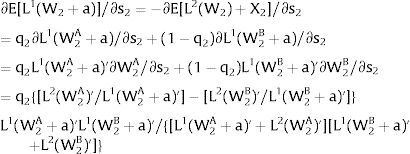
As ∂W2A/∂si>0 (and/or W2B/∂si<0), for si>(<)0,W2A>(<)W2B. On average:
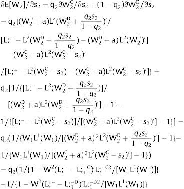
The expected wage responds to uncertainty according to:
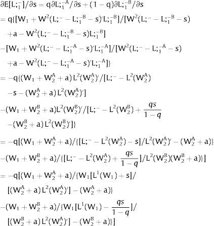
For si>(<)0,W2A>(<)W2B and ∂E[W2]/∂si > (<) 0 if L1(W + a)’ + L2(W)’ rises with W. That occurs when (around a = 0, if the sum of) both labor demands are (is) convex in W – that is, L1(W)” > 0 and L2(W)” > 0. E[W2] decreases with uncertainty (rises with si if positive, decreases if negative) when both (around a = 0, the sum of) labor demands are (is) concave.
Overall, no unemployment is ever generated in the economy. Labor force allocation changes both immediately after a shock, as in expected terms when si rises. When uncertainty rises in region 1:
For s1>(<)0,W2A>(<)W2B and ∂E[L1]/∂s1 > (<) 0 if L1(W + a)’ / L2(W)’ decreases with W.
If it rises in region 2:
For s2>(<)0, W2A>(<)W2B and ∂E[L2]/∂s2 > (<) 0 if L2(W)’ / L1(W + a)’ decreases with W. Around a = 0, that requires that L2(W)” / L2(W)’ < L1(W)” / L1(W)’: E[L2] increases (decreases) with uncertainty in region 2 (rises with s2 if positive, decreases if negative) if the symmetric of the Arrow-Pratt (Arrow, 1965; Pratt, 1964) measure of risk aversion of the local demand (negatively sloped —see section VII below—) is smaller (larger) than that of the other regions.
Remark 1: If at a given level of the argument W, the ratio of marginal values L1(W)’ / L2(W)’ increases with W, the function L1(W) exhibits:
- •
lower risk aversion than the function L2(W), and − L1(W)” / L1(W)’ < − L2(W)” / L2(W)’ when Lj(W)’ > 0.
- •
higher risk aversion than the function L2(W), and L1(W)” / L1(W)’ > L2(W)” / L2(W)’, when Lj(W)’ < 0.
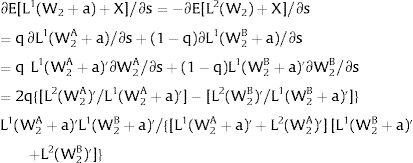
Consider now perfectly and positively correlated uncertainty in the two regions —case 2.b. Then, either s is observed – which occurs with probability q – and
Or, with probability (1 – q), −qs1−q is and:
Wage - W2 - multipliers will double relative to the unilateral uncertainty case – and conclusions remain unaltered.
As for employment:
For s>(<)0, W2A>(<)W2B and ∂E[L1]/∂s > (<) 0 if L2(W)’ / L1(W + a)’ increases with W. Around a = 0, that requires that L2(W)” / L2(W)’ > L1(W)” / L1(W)’: E[L1] increases (decreases) with uncertainty (rises with s if positive, decreases if negative) if the symmetric of the Arrow-Pratt measure of risk aversion of the local – region 1's - demand is smaller (larger) than that of the other regions.
With negatively correlated uncertainty —hypothesis 2.c.—, the wage is invariant to and stabilized at the level for which:
Employment in each region fluctuates mimicking the local shock. Expected local employment does not vary with uncertainty.
Summarizing:
Proposition 2: Under free market, quantity uncertainty and ex-post location flexibility:
2.1. A unilateral or generalized and positively correlated across regions increase in risk will result in a rise (decrease) in the expected “net” wage if the sum of labor demands is convex (concave).
2.2. A unilateral or generalized and positively and perfectly correlated across regions increase in risk will result in a rise (decrease) in the expected employment in a region if the ratio of its labor demand slope to the other region's decreases (increases) with the wage rate, that is, if the symmetric of the Arrow-Pratt measure of risk aversion of the local demand (negatively sloped) is smaller (larger) than that of the other regions.
2.3. Perfectly and negatively correlated labor demand shocks will result in equal employment movements after a shock, neutralizing any effect on the expected wages or local labor force in the economy.
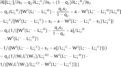
3.1.2Ex-ante location arrangementsConsider case 2.a: only sector i is affected by uncertainty. The labor force settles or affiliates before observing Xi; after, when it makes location changes to region i, it does not know which Xi it is going to face. For equilibrium:
Then, differentiating:
andThe expected wage in the economy moves in the same direction as employment of the region where uncertainty is changing. Employment will flow to the region when local uncertainty rises (decreases) − ∂Li/∂si > (<) 0 when si > 0, ∂Li/∂si < (>) 0 when si < 0 − if Wi(L)” > (<) 0, which occurs, once labor demand is negatively sloped, when Li(W)” > (<) 0, i.e., when labor demand in region i is convex (concave).
Consider case 2.b: both sectors are affected by simultaneous identical shocks. For equilibrium:
Then:
Employment will flow to region 1 when general uncertainty rises (decreases) − ∂L1/∂s > (<) 0 when s > 0, ∂L1/∂s < (>) 0 when s < 0 − if W1(L + g)’ − W2(L;− − L + g)’ increases (decreases) with g, which occurs, once labor demand is negatively sloped, when W1(L)” > W2(L;− − L)” i.e., when inverse labor demand in region 1 is more convex (concave) than that of region 2. As for the wage:
and has the sign of ∂E[W1]/∂s, we expect that the expected wage will rise (decrease) with uncertainty if both inverse demands are convex (concave).Finally, take case 2.c: both regions are affected by simultaneous symmetrical shocks. For equilibrium:
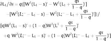
Then, differentiating:
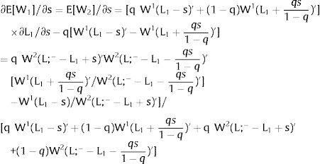
Approximately —through Taylor expansion to the first-order of the terms in the numerator—, ∂L1/∂s > 0 if s > 0 (and ∂L1/∂s < 0 when s < 0), if W1(L1)” > W2(L;− − L1)”: employment rises in the region which has a more convex inverse labor demand.
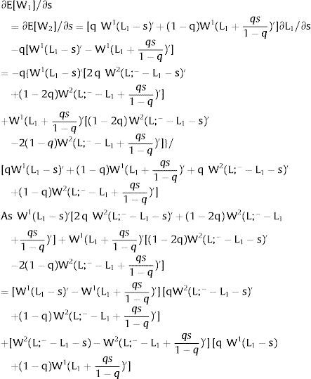
As for the expected wage:
The expected wage increases (decreases) when general uncertainty rises − ∂E[W1]/∂s > (<) 0 when s > 0, ∂E[W1]/∂s < (>) 0 when s < 0 − if W1(L + g)’ / W2(L;− − L − g)’ decreases (increases) with g – or, equivalently, if W1(L + g)’ W2(L;− − L + g)’ decreases (increases) with g. That occurs, around g = 0, when W1(L)” / W1(L)’ + W2(L;− − L)” / W2(L;− − L)’ < (>) 0 – the sum of the symmetric of the Arrow-Pratt measures of risk aversion of the inverse demands (that symmetric measuring their concavity) —is smaller (larger) than 0—.
Remark 2: If the product of the marginal values of two functions of the same argument, W1(L)’ W2(L)’, increases with it, the sum of the corresponding absolute risk aversion measures:
- •
is negative and − W1(L)” / W1(L)’ − W2(L)” / W2(L)’ < 0 when Wj(L)’ > 0.
- •
is positive and W1(L)” / W1(L)’ + W2(L)” / W2(L)’ > 0 when Wj(L)’ < 0.
Proposition 3: Under free market, subject to quantity uncertainty and to ex-ante location decisions:
3.1. A unilateral increase in risk will result in a rise (decrease) in the expected wages and employment in the affected region if its labor demand is convex (concave).
3.2. A generalized and perfectly correlated across regions increase in risk will result in a rise (decrease) in the expected employment in the region of more convex (concave) inverse labor demand.
3.3. A generalized and positively and perfectly correlated across regions increase in risk will result in a rise (decrease) in the expected wages if both labor demands are convex (concave).
3.4. Perfectly and negatively correlated labor demand shocks will result in a rise (decrease) in the expected wages if the sum of the symmetric of the Arrow-Pratt measures of risk aversion of the inverse labor demands is negative (positive).
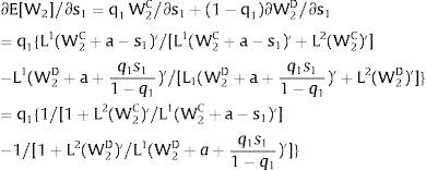
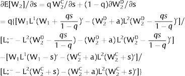
3.2Productivity uncertainty3.2.1Ex-post flexibilityConsider case 2.a: only region i, is affected by uncertainty, implying a noise around the observed wage distribution – subtracted from the local expected or average wage.
Let 1 be the region affected by uncertainty. Either s1 is observed – which occurs with probability q1 – and
Then:
Or, with probability (1 – q1), −q1s11−q1 is and:
and
As ∂W2C/∂s1>0 (and/or ∂W2D/∂s1<0), for s1>(<)0,W2C>(<)W2D. On average:
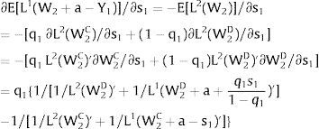
Overall, no unemployment is ever generated in the economy. When uncertainty rises in region 1:
If it rises in region 2, we would have analogous conclusions. Let us define the problem in terms of inverse demands: either s2 is observed – which occurs with probability q2 – and
Then:
Or, with probability (1 – q2), −q2s21−q2 is and:
and∂L2D/∂s2=q21−q2/[W1(L;−−L2D)'+W2(L2D)']<0
As ∂L2C/∂s2>0 (and/or ∂L2D/∂s2<0), for s2>(<)0,L2C>(<)L2D. On average:
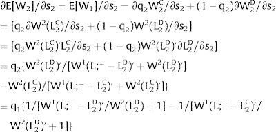
For s2>(<)0,L2C>(<)L2D and ∂E[L2]/∂s2 > (<) 0 if W1(L;− − L)’ + W2(L)’ rises with L. That requires that W2(L)” > W1(L;− − L)”: E[L2] increases with uncertainty in region 2 (rises with s2 if positive, decreases if negative) if the inverse demand in region 2 is more convex than the first one.
Overall, no unemployment is ever generated in the economy. As for the baseline region 2's wage:
For s2>(<)0,L2C>(<)L2D and ∂E[W2]/∂s2 > (<) 0 if W2(L)’ / [W1(L;− − L)’ + W2(L)’] decreases with L – or, equivalently, W2(L)’ / W1(L;− − L)’ decreases with L. That requires that W2(L)” / W2(L)’ + W1(L;− − L)” / W1(L;− − L)’ < 0: E[W2] increases with uncertainty in region 2 (rises with s2 if positive, decreases if negative) when the sum of the symmetric of the Arrow-Pratt measures of risk aversion of the inverse demands (negatively sloped) is negative (this occurs if both inverse - and direct, once they are negatively sloped - demands are convex). It decreases when that sum is positive.
Consider now perfectly and positively correlated uncertainty in the two regions - case 2.b. Then, either s is observed – which occurs with probability q – and
Or, with probability (1 – q), −qs1−q is and:
Then:
Employment is always stabilized after a shock – local employment remains constant after a realization of Y. Hence:
With negatively correlated uncertainty – hypothesis 2.c. -, either s is observed – which occurs with probability q – and:
oror −qs1−q is observed – which occurs with probability (1 – q) – and:
Obviously, the multipliers double with respect to unilateral uncertainty surrounding only one region and the consequences of a rise in uncertainty are the same: E[Li] increases with uncertainty (rises with s if positive, decreases if negative) when the inverse demand of region i is more convex than that of region j's.
E[W2] and E[W1] increase with uncertainty (rises with s if positive, decreases if negative) when the sum of the symmetric of the Arrow-Pratt measures of risk aversion of the inverse demands (negatively sloped) is negative (this occurs if both inverse - and direct, once they are negatively sloped - demands are convex).
Summarizing:
Proposition 4: Under free market, productivity uncertainty and ex-post location decisions:
4.1. A unilateral or generalized and negatively correlated across regions increase in risk will result in a rise (decrease) in the expected employment of the region with more convex (concave) inverse labor demand. Expected wages will rise (decrease) with such uncertainty if the sum of relative concavity (measured by the symmetric of the Arrow-Pratt measure of risk aversion) of the inverse demand functions is negative (positive).
4.2. Perfectly and positively correlated wage shocks will result in equal wage movements, neutralizing any effect on the expected wages or local labor force of the economy.
3.2.2Ex-ante location arrangementsProductivity dispersion has no effect on the expected equilibrium if ex-ante decisions regarding quantities must be made.
Proposition 5: Under free market, productivity uncertainty, and ex-ante decisions, labor market outcomes are invariant to dispersion in the wage distribution.
4Partial coverage - The perfect mobility caseAssume 3.a, 4.b and 5.a. of section I. The wage in the two regions differ potentially by more than a. In region 1, the wage is fixed at level W1. As the other region's wage is free, it will decrease till all the labor force is employed.
Under constrained wages in sector 1 and free mobility, expected wage equalization may, therefore, never be fulfilled. Then the compensating differential does not have a specific meaning – we can consider it added to form the institutional W1, or that the resulting equilibrium wage differential is already sufficient to compensate for it – i.e., naturally larger than a: the equilibrium wage of region 2, W2 < W1 – a for the minimum wage to be a binding restriction. Otherwise, we fall into the case of section II.
Proposition 6: 6.1. In a dualistic model with perfect mobility and institutional wage fixed in one of the sectors, the equilibrium wage in the second sector is lower than the free market wage. There will be no unemployment.
6.2. An increase in local externalities favouring one of the regions will have either no effect or render the institutional wage barrier inactive.
4.1Quantity uncertainty4.1.1Ex-post flexibilityConsider case 2.a: only sector i is affected by uncertainty.
Either si is observed – which occurs with probability qi – and
Then:
Or, with probability (1 – qi), −qisi1−qi is and:
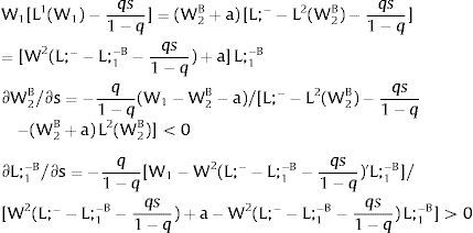
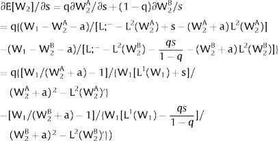
andAs ∂W2A/∂si>0 (and/or ∂W2B/∂si<0), for si>(<)0, W2A>(<)W2B. On average:
For si>(<)0,W2A>(<)W2B and ∂E[W2]/∂si > (<) 0 if L2(W)’ rises with W. That occurs when the uncovered sector labor demand is convex – that is, L2(W)” > 0. E[W2] decreases with uncertainty (rises with si if positive, decreases if negative) when the uncovered region labor demand is concave.
Overall, no unemployment is ever generated in the economy. Labor force allocation changes only aftershocks in sector 1 - and by the same magnitude. As E[Xi] = 0, a rise in si has no effect on expected local employment:
and:Consider now perfectly and positively correlated uncertainty in the two regions - case 2.b. Then, either s is observed – which occurs with probability q – and
Or, with probability (1 – q), −qs1−q is and:
Multipliers will double relative to the unilateral uncertainty case – and conclusions remain unaltered.
As for employment, again:
With negatively correlated uncertainty – hypothesis 2.c. -, the wage is invariant to and stabilized at the level for which:
Employment in each region fluctuates mimicking the local shock. Expected local employment does not vary with uncertainty.
Summarizing:
Proposition 7: In a dualistic model with perfect mobility and institutional wage fixed in one of the regions, under quantity uncertainty and ex-post location flexibility:
7.1. A unilateral or generalized and positively correlated across regions increase in risk will result in a rise (decrease) in the expected “net” wage if the uncovered region labor demand is convex (concave).
7.2. A unilateral or generalized and perfectly correlated across regions increase in risk will have no effect on expected local employment.
7.3. Perfectly and negatively correlated labor demand shocks will result in equal employment movements, neutralizing any effect on the expected wages in the economy.
4.1.2Ex-ante location arrangementsEx-ante location arrangements would be problematic to model under perfect mobility when uncertainty in covered region 1 is staged: unemployment would necessarily be generated. If we consider this a possibility, and allow for (uncorrelated) uncertainty also in region 2, the general equilibrium for s1 > 0 can be written as:
Yet, if there is uncertainty in region 2, it may be worthwhile to face unemployment chances in region 1 even when the shock is positive:
Then we fall into the imperfect mobility environment of the next Section, IV. We therefore discard the possibility, consider case 2.a, and that only sector 2 is affected by uncertainty. Always:
andThe expected wage in region 2 rises (decreases) with local uncertainty − ∂E[W2]/∂s2 > (<) 0 when s2 > 0, ∂E[W2]/∂s2 < (>) 0 when s2 < 0 − if W2(L)” > (<) 0, which occurs, because labor demand is negatively sloped, when L2(W)” > (<) 0 i.e., when labor demand in region 2 is convex (concave).
As L1(W1) is fixed, also is the labor force. The effect of a rise in its volatility is nil:
Proposition 8: In a dualistic model with perfect mobility and institutional wage fixed in one of the regions, subject to quantity uncertainty and to ex-ante decisions:
8.1. A unilateral increase in risk in the uncovered sector will result in a rise (decrease) in the expected “net” wage if the uncovered sector labor demand is convex (concave).
8.2. An increase in risk in the covered region will lead to an imperfect mobility stage.
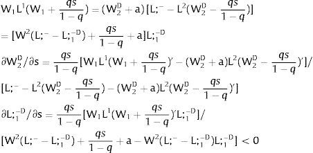
4.2Productivity uncertainty4.2.1Ex-post flexibilityConsider case 2.a: only one region is affected by uncertainty. Conclusions differ according to which region is affected by Y.
Either s1 is observed – which occurs with probability q1 – and
Then:
Or, with probability (1 – q1), −q1s11−q1 is and:
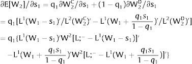
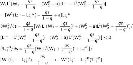
andAs ∂W2C/∂s1>0 (and/or ∂W2D/∂s1<0),for s1>(<)0, W2C>(<)W2D. On average:
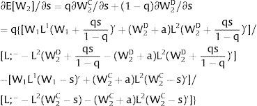
∂E[W2]/∂s1 > (<) 0 when s1 > 0 − ∂E[W2]/∂s1 < (>) 0 when s1 < 0 −, if L1(W)’ W2[L;− −L1(W)]’ decreases (increases) with W. That occurs when L1(W)” / L1(W)’ < (>) L1(W)’ W2[L;− −L1(W)]” / W2[L;− −L1(W)]’ – when the symmetric of the Arrow-Pratt measure of risk-aversion of region 1's labor demand is smaller (larger) than the same measure for the uncovered region inverse demand multiplied by the covered region labor demand slope. That is equivalent – using Remark 4 of section VII below – to have W1(L)” / W1(L)’ + W2[L;− −L1(W)]” / W2[L;− −L1(W)]’ < (>) 0.
∂E[L1(W1 – Y)]/∂s1 > (<) 0 when s1 > (<) 0 if L1(W)” > 0: expected employment rises in region 1 if its local labor demand is convex.
When 2 is the affected region: either s2 is observed – which occurs with probability q2 – and
Then:
Or, with probability (1 – q2), −q2s21−q2 is and:
andAs ∂W2C/∂s2>0 (and/or W2D/∂s2<0), for s2>(<)0, W2C>(<)W2D. On average:
As W1 is fixed, also L1(W1) and labor force allocation is invariant to uncertainty:
Given this, the effect of compound uncertainty in both sectors – that is, if we staged 2.b or 2.c. – we always conclude about a rise in risk as for expected wages or employment after the unilateral change in s1.
Proposition 9: In a dualistic model with perfect mobility and institutional wage fixed in one of the regions, under productivity uncertainty and ex-post location flexibility:
9.1. A unilateral increase in wage dispersion in the uncovered region will have no effect on expected wage or local employment.
9.2. A unilateral increase in risk in the covered region or generalized and perfectly correlated increase in productivity dispersion across regions will result in a rise (decrease) in the expected wage if the sum of the symmetric of the Arrow-Pratt measure of risk-aversion of the inverse labor demands is negative (positive); in a rise (fall) in the covered sector's employment if the covered sector labor demand is convex (concave).
4.2.2Ex-ante location arrangementsAgain, as we are assuming perfect mobility, that ex-ante location decisions are fixed becomes an awkward hypothesis: we would always have access to the other sector's jobs – then we could recover the ex-post mobility result.
The general equilibrium for s1 > 0 can be written as:
If it becomes worthwhile to face unemployment chances in sector 1 even when the shock is positive:
Then we fall into the imperfect mobility environment of the next section, IV.
Consider then case 2.a and that only region 2 is affected by uncertainty. As
productivity uncertainty has no effect on expected outcomes, once it only affects the uncovered region wage and in an additive fashion.
Proposition 10: In a dualistic model with perfect mobility and institutional wage fixed in one of the regions, subject to productivity uncertainty and to ex-ante decisions:
10.1. A unilateral increase in risk in the uncovered region will have no effect on employment allocation or expected wage.
10.2. An increase in risk in the covered region will lead to an imperfect mobility stage.
5Partial coverage and imperfect mobility - The Harris-Todaro modelAssume 3.b, 4.b and 5.a. of section I. The wage in the two regions differs. In region 1, the net wage is fixed at level W1.
As region 2's wage is free, it will decrease till all the local labor force is employed:
However, to have access to wage W1, people have to locate there, or to specialize if we are addressing industry rather than regional affiliation – implying that unemployment will be generated in the region. There will be labor force flows till
W1 x Probability of Employment in region 1 = W2 + a
That is, in the long run we expect that:
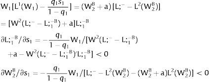
orthe wage bill – and the expected wage in the economy – will increase (decrease) with a if the absolute value of the elasticity of labor demand in region 2 is larger than 1. (Aggregate workers’ welfare, W1 L1 + (W2 + a) L2 = (W2 + a) L;−, will always increase with a.)
Proposition 11: 11.1. Consider a dualistic model with imperfect mobility in the short-run. The equilibrium wage in the second sector may be higher or lower than the free market equilibrium, and there will be unemployment in the institutional sector or urban region.
11.2. An increase in local externalities favouring the uncovered (covered) region will attract the labor force to the latter and depress the local (raise the uncovered regions) wage. The average wage in the economy will increase (decrease) if the absolute value of the elasticity of labor demand in covered region exceeds (is smaller than) 1.
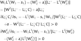
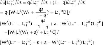
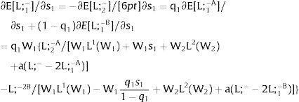
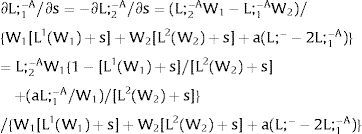
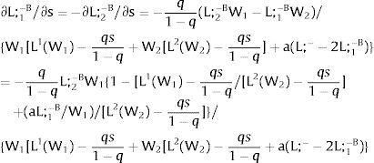
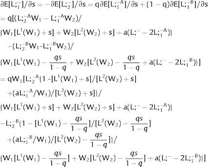
5.1Quantity uncertainty5.1.1Ex-post flexibilityLet us consider 2.a. Assume X2 = 0: uncertainty only afflicts covered region 1's employment. Then:
Either s1 is observed – which occurs with probability q1 – and
Or, with probability (1 – q1), −q1s11−q1 is and:
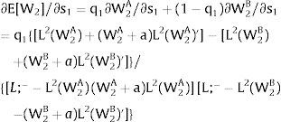
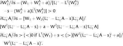
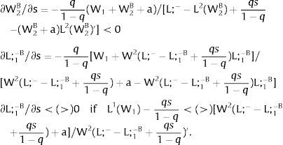
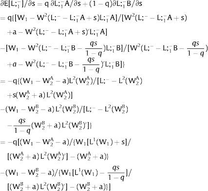
As ∂W2A/∂s1>0 (and/or ∂W2B/∂s1<0), for s1>(<)0, W2A>(<)W2B. On average:
For s1>(<)0,W2A>(<)W2B and ∂E[W2]/∂s1 > (<) 0 if [L2(W) + (W + a) L2(W)’] rises with W. Around a = 0, that occurs when the uncovered region wage bill function, [W L2(W)], is convex in W. E[W2] decreases with uncertainty (rises with s1 if positive, decreases if negative) when the uncovered region's wage bill is concave in W.
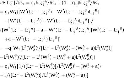
As ∂L;1−A/∂s1>0 (and/or ∂L;1−B/∂s1<0), for s1>(<)0, L;1−A>(<) L;1−B. On average:
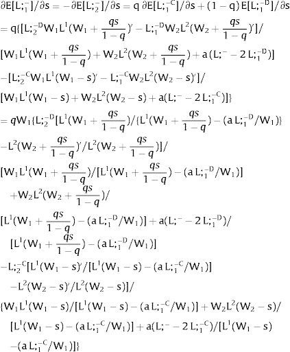
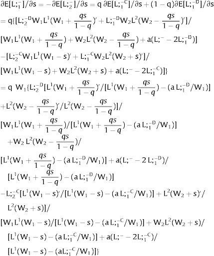
For s1>(<)0, L;1−A>(<) L;1−B and ∂E[L;1−]/∂s1>(<)0 if W2(L;− − L) − W2(L;− − L)’ L decreases with L. That occurs when the uncovered region wage times the other region's employment, [W2(L;− − L) L], is concave in L. E[L;−1] decreases with uncertainty (rises with s1 if positive, decreases if negative) when [W2(L;− − L) L] is convex in L. Referring to L;2−A<(>)L;2−B if s1>(<)0,∂E[L;1−]/∂s1>(<)0. if W2(L) − W2(L)’ (L;− − L) increases (decreases) with L – if [W2(L) (L;− − L)] is concave (convex) in L.
Equivalently, around a=0,L;1− will rise (decrease) with uncertainty if [L;− − L2(W)] / L2(W)’ + W increases (decreases) with W.
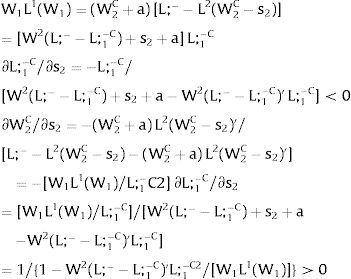
Let now be region 2 suffering uncertainty and X1 = 0. For s2 – which occurs with probability q2 – and
With probability (1 – q2), −q2s21−q2 is observed and:
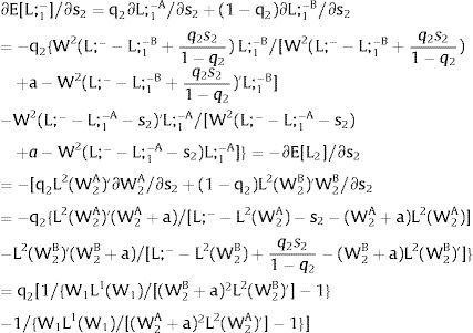
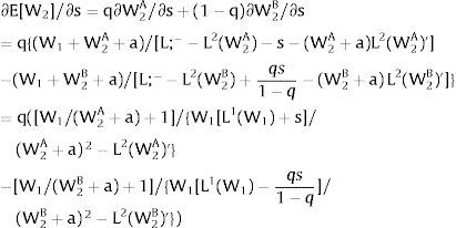
As ∂W2A/∂s2>0 (and/or W2B/∂s2<0), for s2>(<)0, W2A>(<)W2B. On average, around a = 0:
For s2>(<)0,W2A>(<)W2B and ∂E[W2]/∂s2 > (<) 0 if L2(W)’− W1L1(W1)/W2 rises with W. That occurs when the total wage bill divided by the uncovered region's wage is convex in it – that is, if d2{[W1 L1(W1) + W L2(W)] / W}/dW2 > 0. E[W2] decreases with uncertainty (rises with s2 if positive, decreases if negative) when that ratio is concave.
As ∂L;1−A/∂s2<0 (and/or ∂L;1−B/∂s2>0), for s2>(<) 0, L;1−A<(>)L;1−B. On average:
For s2>(<)0,W2A>(<)W2B and, around a = 0, ∂E[L2]/∂s2 > (<) 0 if L2(W)’ W2 rises (decreases) with W.
Taking 2.b., and allowing for perfectly and positively correlated uncertainty we derive that:
Either s is observed – which occurs with probability q – and
Then:
Or, with probability (1 – q), −qs1−q is and:
As ∂W2A/∂s>0 (and/or ∂W2B/∂s<0), for s>(<) 0, W2A>(<)W2B. On average:
For s>(<)0,W2A>(<)W2B and ∂E[W2]/∂s > (<) 0 if but not only if [L2(W) + (W + a) L2(W)’] rises with W. Around a = 0, that occurs – E[W2] rises with uncertainty - when the uncovered region wage bill function, [W L2(W)], is convex.
For s>(<)0,W2A>(<)W2B and ∂E[W2]/∂s < (>) 0 around a = 0 if but not only if W1L1(W1)/W2 − L2(W)’ rises with W. That occurs, and E[W2] decreases with uncertainty when the total wage bill divided by the uncovered region's wage is concave in it – that is, if d2{[W1 L1(W1) + W L2(W)] / W}/dW2 < 0.
On average:
For s>(<)0,W2A>(<)W2B; ∂E[L2]/∂s>(<)0 and L2 rises with uncertainty if but not only if [(W + a) L2(W)’] rises with W.
Finally, for 2.c., and with perfectly negatively correlated uncertainty in the regions we derive that:
Either s is observed – which occurs with probability q – and
Then:
Or, with probability (1 – q), −qs1−q is and:
As ∂W2A/∂s>0 (and/or ∂W2B/∂s<0), for s>(<) 0, W2A>(<)W2B. On average:
For s>(<) 0,W2A>(<)W2B and ∂E[W2]/∂s < (>) 0 if but not only if [L2(W) + (W + a) L2(W)’] decreases with W. Around a = 0, that occurs when the uncovered sector wage bill function, [W L2(W)], is concave. Or:
For s>(<) 0, W2A>(<)W2B and ∂E[W2]/∂s < (>) 0 around a = 0 if but not only if W1L1(W1)/W2−L2(W)’ rises with W. That occurs, and E[W2] decreases with uncertainty if but not only if the total wage bill divided by the uncovered region's wage is concave in it – that is, if d2{[W1 L1(W1) + W L2(W)] / W}/dW2 < 0.
There will be a composition of effects but sign directions are not so definite.
Proposition 12: Consider a dualistic model with imperfect mobility in the short-run. Under quantity uncertainty and ex-post location flexibility:
12.1. A unilateral increase in risk in the covered sector will result in a rise (decrease) in the expected “net” wage if the uncovered sector's wage bill is convex (concave). Expected local labor force increases (decreases) with uncertainty if the inverse demand of the uncovered sector multiplied by excess employment relative to total supply is concave (convex) in L.
12.2. A unilateral increase in risk in the uncovered sector will result in a rise (decrease) in the expected wage if the total wage bill divided by the uncovered sector's wage is convex (concave) in it. Expected local labor force increases (decreases) with uncertainty if the slope of the uncovered sector's demand multiplied by the square of the wage increases (decreases) with the latter.
12.3. A perfectly and positively correlated across regions increase in risk will result in a rise in the expected wage if but not only if the uncovered sector's wage bill is convex; a fall if but not only if the total wage bill divided by the uncovered sector's wage is concave in it. Expected labor force in the uncovered sector increases with uncertainty if the slope of the uncovered sector's demand multiplied by the wage rate increases with it.
12.4. A perfectly and negatively correlated across regions increase in risk will result in a decrease in the expected wage if but not only if the uncovered sector's wage bill is concave; or if but not only if the total wage bill divided by the uncovered sector's wage is concave in it.
5.1.2Ex-ante location arrangementsThe expected wage bill in region 1 is fixed. Hence, only the uncertainty affecting region 2's wage has an impact on the labor force allocation:
Then:
For s2>(<) 0,W2(L;−−L;1−−s2)'>(<)W2(L;−−L;1−+q2s21−q2)' and ∂L;1−/∂s2>(<) 0 and ∂L;2−/∂s2<(>) 0 − if W2(L)’ decreases (rises) with L: when the uncovered region inverse demand is concave (convex) in L – and the labor demand function L2(W), is concave (convex) in W.
The expected wage will move in opposite direction to the labor force in the covered region.
Proposition 13: With multiple coverage and imperfect mobility, quantity uncertainty with ex-ante location decisions.
13.1. A unilateral increase in risk in the covered region will have no effect on employment allocation or expected wage.
13.2. An increase in risk in the uncovered region will result in an increase (decrease) in the local labor force and of the expected wage in the economy if the uncovered region labor demand is convex (concave).
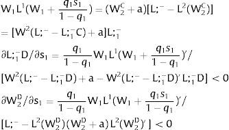
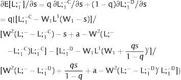
5.2Productivity uncertainty5.2.1Ex-post flexibilityIn general, the equilibrium satisfies:
Let Y2 = 0: uncertainty only afflicts covered region 1's employment. Then:
Either s1 is observed – which occurs with probability q1 – and
Or, with probability (1 – q1), −q1s11−q1 is and:
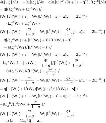
As ∂W2C/∂s1>0 (and/or ∂W2D/∂s1<0),for s1>(<) 0,W2C>(<)W2D. On average:
For s1>(<) 0,W2C>(<)W2D and ∂E[W2]/∂s1 > (<) 0 if [L2(W) + (W + a) L2(W)’] rises with W – provided L1(W1) is not too concave. Around a = 0, that occurs when the uncovered region wage bill function, [W L2(W)], is convex. E[W2] decreases with uncertainty (rises with s1 if positive, decreases if negative) when the uncovered wage bill is concave – provided L1(W1) is not too convex.
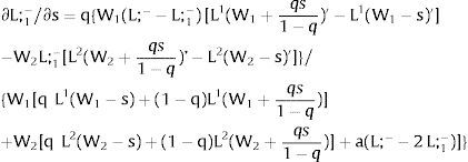
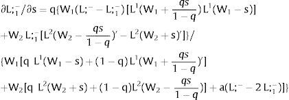
As ∂L;1−C/∂s1>0 (and/or ∂L;1−D/∂s1<0),for s1>(<) 0,L;1−C>(<) L;1−D. On average:
For s1>(<) 0,L;1−C>(<) L;1−D and ∂E[L;1−]/∂s1>(<) 0 if W2(L;−−L)−W2(L;−−L)'L decreases with L; or W2(L)−W2(L)'(L;−−L) increases with L− provided that L1W1 is not too concave. That occurs when the uncovered region wage times the other region's employment [W2(L;−−L)L], is convex in L− if W2(L)(L;−−L) is concave in L. E [L;1−] decreases with uncertainty (decreases with s1 if positive, increases if negative) when [W2(L;−−L)L] is concave in L− if W2(L)(L;−−L) is convex in L− provided L1(W1) is not too convex.
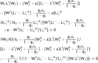
Let now be region 2 suffering uncertainty and Y1=0. For s2− which occurs with probability q2− and
With probability (1−q2),−q2s21−q2 is observed and:
As ∂W2C/∂s2>0 (and/or ∂W2D/∂s2<0), for s2>(<)0,W2C>(<)W2D. On average:
For s2>(<) 0,L;1−C<(>)L;1−D and ∂E[W2]/∂s2>(<)0if[W2(L;−−L)'L2] decreases with L− or if [W2(L)'(L;−−L)2] increases with L.E[W2] decreases with uncertainty (decreases with s2 if positive, increases if negative) when [W2(L;−−L)'L2] increases with L−[W2(L)'(L;−−L)2] decreases with L.
As ∂L;1−C/∂s2<0 (and/or ∂L;1−D/∂s2>0), for s2>(0<) 0,L;1−C<(>) L;1−D. On average:
For s2>(<) 0,L;1−C<(>)L;1−D and ∂E[L;1−]/∂s2>(<) 0 if W1L1(W1)/L2−W2(L;−−L)' decreases with L. That occurs when the ratio [W1L1(W1)−W2(L;−−L)L]/L is convex in L, i.e., d2{[W1L1(W1)−W2(L;−−L)L]/L}/dL2>0. E[L;1−] decreases with uncertainty (rises with s2 if positive, decreases if negative) when that ratio is concave.
Taking 2.b., and allowing for perfectly and positively correlated uncertainty we derive that:
Either s is observed – which occurs with probability q – and
Then:
Or, with probability (1−q),−qs1−q is and:
As ∂W2C/∂s>0 (and/or W2D/∂s<0), for s>(<)0,W2C>(<)W2D. On average:
∂L;1−C/∂s>0 (and/or ∂L;1−D/∂s<0), and L;1−C>(<)L;1−D for s>(<)0, if, approximately, the absolute value of the wage elasticity of the uncovered region's demand is larger than 1. ∂L;1−C/∂s<0 (and/or ∂L;1−D/∂s>0), for s>(<)0, and L;1−C<(>) L;1−D if, approximately, the absolute value of the wage elasticity of the uncovered region's demand is smaller than 1. On average:
Finally, for 2.c., and with perfectly negatively correlated uncertainty in the sectors we derive that:
Either s is observed – which occurs with probability q – and
Then:
Or, with probability (1−q), qs1−q is and:
∂W2C/∂s>0 (and/or ∂W2D/∂s<0) and W2C>(<)W2D for s>(<)0, if, approximately, if the absolute value of the wage elasticity of the uncovered region's demand is larger than 1. ∂W2C/∂s<0 (and/or W2D/∂s>0) and W2C<(>)W2D for s>(<)0 if, approximately, if the absolute value of the wage elasticity of the uncovered region's demand is smaller than 1. On average:
As ∂L;1−C/∂s>0(and/or ∂L;1−D/∂s<0),for s>(<)0,L;1−C>(<)L;1−D. On average:
Proposition 14: In dualistic model with imperfect mobility in the short-run, under productivity uncertainty and ex-post location flexibility:
14.1. A unilateral increase in risk in the covered region will result in a rise (decrease) in the expected “net” wage if the uncovered region's wage bill is convex (concave). Expected local labor force increases (decreases) with uncertainty if the inverse demand of the uncovered region multiplied by excess employment relative to total supply is concave (convex) in L.
14.2. A unilateral increase in risk in the uncovered region will result in a rise (decrease) in the expected wage if the slope of the uncovered region's inverse demand multiplied by the square of the excess employment relative to total labor supply increases (decreases) with employment. Expected local labor force increases (decreases) with uncertainty if the ratio [W1 L1(W1) − W2(L;− − L) L] / L is concave (convex) in L.
14.3. A perfectly correlated across regions increase in risk will result in a composite of the unilateral effects – a sum if positive, a difference if negative.
5.2.2Ex-ante location arrangementsThe expected wage bill in region 2 is constant, once uncertainty is additive to the wage. Hence, only the uncertainty affecting region 1's productivity has an impact on the labor force allocation:
Then:
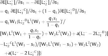
For s1 > (<) 0, L1(W1 + q1s11−q1)’ > (<) L1(W1 – s1)’ and ∂L;1− / ∂s1 > (<) 0 if L1(W)’ increases with W: ∂L;1− increases with uncertainty when the covered region labor demand is convex in W. For s1 > (<) 0, ∂L;1− / ∂s1 < (>) 0 if the covered region labor demand is concave in W.
The expected wage will move in the same direction as the labor force in the covered region.
Proposition 15: With multiple coverage and imperfect mobility, productivity uncertainty with ex-ante location decisions.
15.1. A unilateral increase in risk in the uncovered region will have no effect on employment allocation or expected wage.
15.2. An increase in risk in the covered region will result in an increase (decrease) in the local labor force and of the expected wage in the economy if the covered region labor demand is convex (concave).
6Multiple or global coverage under imperfect mobility - The Bhagwati-Hamada modelAssume 3.b, 4.b. and 5.b. of section I. The wages are fixed in both regions, at levels Wi, i =1,2. One can see this same (technically speaking) scenario in, for example, Bhagwati and Hamada (1974).
Equilibrium is defined by:
The average wage in the economy [W1 L1(W1) + W2 L2(W2)]/ L;− is fixed.
Differentiating (68):
Proposition 16: 16.1. With multiple coverage and imperfect mobility, both regions will experience unemployment and expected “net” wage is equalized across regions. The average wage in the economy does not change with a local differential, once the wage bill is fixed. Also:
16.2. An increase in the local differential favouring one of the regions will attract the labor force to it. Local expected wage will decrease there and rise – as well as the expected worker's welfare - in the other sector.
6.1Quantity uncertainty6.1.1Ex-post flexibilityThen, local employment, being demand determined:
Equilibrium is defined by:
If a is 0, one can show that the expected wage in the economy will equal the wage bill divided by L;−: {W1 [L1(W1) + X1] + W2 [L2(W2) + X2]} / L;−. Additive uncertainty will have then no effect on the equilibrium expected wage.
One can re-write condition (166) as:
Consider case 2.a: only region i is affected by uncertainty and Xj = 0. For equilibrium:
Either s1 is observed – which occurs with probability q1 – and
Or, with probability (1 – q1), −q1s11−q1 is and:
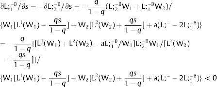
As ∂L;1−A/∂s1>0(and/or ∂L;1−B/∂s1<0), for s1>(<)0,L;1−A>(<)L;1−B. On average:
As L;1−A>(<)L;1−B – and L;2−A<(>)L;2−B − for s1 > (<) 0, ∂E[L;1−]/∂s1<(>)0 around a = 0: expected labor force flows away from the region where uncertainty rises.
Let there be case 2.b: Xi = Xj = X. In equilibrium:
Either s is observed – which occurs with probability q – and
∂L;1−A/∂s>0, and, for s>(<)0,L;1−A>(<)L;1−B,if L2(W2)>L1(W1) – after a generalized positive shock, the labor force flies away from the region of higher aggregate demand – proportionately, the other becomes more appealing.
Or, with probability (1 – q), −qs1−q is and:
Then:
As ∂L;1−A/∂s>0(∂L;1−B/∂s<0), for s>(<)0,L;1−A>(<)L;1−B if L2(W2) > L1(W1), given that then [L1(W1) +s] / [L2(W2) +s] increases with s, being larger (smaller) than [L1(W1) −qs1−q] / [L2(W2) −qs1−q] for s > (<) 0, we conclude that ∂E[L;1−]/∂s<(>)0 for s > (<) 0, if L2(W2) > L1(W1). Also, ∂E[L;1−]/∂s>(<)0 for s > (<) 0, if L2(W2) < L1(W1). After a rise in uncertainty, the labor force will shift away from the region of smaller aggregate demand.
Let there be case 2.c: Xi = − Xj = − X. In equilibrium:
Either s is observed – which occurs with probability q – and
Or, with probability (1 – q), −qs1−q is and:
Then:
If W1 > W2, one can show that – around a=0−L;2−A/[L2(W2)−s] decreases with s. Then, for s>0,∂E[L;1−]/∂s<0; for s<0,∂E[L;1−]/∂s>0. If W1 < W2, s > (<) 0, ∂E[L;1−]/∂s>(<)0
Proposition 17: With multiple coverage and imperfect mobility, under quantity uncertainty and ex-post location flexibility:
17.1. The expected (or average) wage in the economy does not change with uncertainty.
17.2. A unilateral increase in risk will result in a flight of labor force out of the inflicted region.
17.3. A generalized and positively correlated across regions increase in risk will result in a flow of labor force out of the region with smaller aggregate employment.
17.4. A rise in perfectly and negatively correlated labor demand uncertainty will result in a flow of labor force out of the region with highest wage.
6.1.2Ex-ante location arrangementsProposition 18: With multiple coverage and imperfect mobility, quantity uncertainty with ex-ante location decisions render labor force allocation and expected wages invariant to uncertainty.
6.2Productivity uncertainty6.2.1Ex-post flexibilityThen, local employment, being demand determined:
Equilibrium is defined by:
One can re-write condition (73) as:
As, for a = 0, the expected wage in the economy equals the wage bill divided by L;−: {W1 L1(W1 − Y1) + W2 L2(W2 – Y2)} / L;−, the expected wage in the economy rises with uncertainty if at least one of the demands the argument of which is random is sufficiently convex.
Consider case 2.a: only region i is affected by uncertainty and Y2 = 0. For equilibrium:
Either s1 is observed – which occurs with probability q1 – and
Or, with probability (1 – q1), −q1s11−q1 is and:
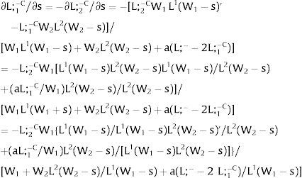
As ∂L;1−C/∂s1>0 (and/or ∂L;1−D/∂s1<0), for s1>(<) 0, L;1−C>(<)L;1−D. On average:
Expected labor force flows away from the region where uncertainty rises, provided local labor demand is not too convex.
Let there be case 2.b: Yi = Yj = Y. In equilibrium:
Either s is observed – which occurs with probability q – and
∂L;1−C/∂s>0, and, for s>(<)0,L;1−C>(<)L;1−D, if L1(W1−s)'/L1(W1−s)
Or, with probability (1 – q), −qs1−q is and:
Then:
When ∂L;1−C/∂s>0, and, for s >(<)0,L;1−C>(<)L;1−D, and L1(W1−s)'/L1(W1−s)
Let there be case 2.c: Yi = − Yj = − Y. In equilibrium:
Either s is observed – which occurs with probability q – and
Or, with probability (1 – q), −qs1−q is and:
As ∂L;1−C/∂s > 0 (and ∂L;1−D/∂s < 0), for s > (<) 0, L;1−C > (<) L;1−D. Then:
As ∂L;1−C/∂s>0, and, for s>(<)0, L;1−C>(<)L;1−D. A definite pattern for how E[L;−] responds to uncertainty is unclear.
Proposition 19: With multiple coverage, under productivity uncertainty and ex-post location flexibility.
19.1. A unilateral increase in risk will result in a flight of expected labor force out of the inflicted region provided the local demand is not too convex. Expected wage in the economy will rise (decrease) if the demand of the affected region is convex (concave).
19.2. A generalized and positively correlated across regions increase in risk will result in a flow of labor force out of the region with highest semi-elasticity of labor demand in absolute value, if (but not only if) this increases more rapidly than the other's. The expected wage will increase (decrease) with risk if convexity (concavity) of the weighted (by wage) sum of the labor demands dominates.
19.3. A rise in perfectly and negatively correlated labor demand uncertainty will result in a flow difficult to determine. The expected wage will increase (decrease) with risk if convexity (concavity) of the weighted (by wage) sum of the labor demands dominates.
6.2.2Ex-ante location arrangementsConsider case 2.a: only region i is affected by uncertainty and Yj = 0. For equilibrium:
Then:
Employment will flow to (out of) a region where uncertainty rises if the local demand of the latter is convex (concave).
Consider case 2.b: both sectors are affected by positively correlated uncertainty. For equilibrium:
Then:
∂L;1−/∂s>0 for s>0 if W1(L;−−L;1−) [L1(W1+qs1−q)'−L1(W1−s)']>[L2(W2+qs1−q)'−L2(W2−s)']W2L;1−. Around a = 0, that is equivalent to [L1(W1 + qs1−q)' − L1(W1 – s)’] / [q L1(W1 – s) + (1 –q) L1(W1 + qs1−q)] > [L2(W2 + qs1−q)' − L2(W2 – s)’] / [q L2(W2 – s) + (1 –q) L2(W2 + qs1−q)]. That occurs approximately for L1(W1)” / L1(W1) > L2(W2)” / L2(W2). ∂L;−1/∂s < 0 for s > 0 when L1(W1)” / L1(W1) < L2(W2)” / L2(W2). Then, the labor force will flow to the region of more relatively (to its aggregate size) convex labor demand.
Finally, let case 2.c: both regions are affected by negatively correlated uncertainty. For equilibrium:
Then:
∂L;1−/∂s>0 for s>0 if W1L;2−[L1(W1+qs1−q)'−L1(W1−s)']>W2L;1−[L2(W2+s)'−L2(W2−qs1−q)']. Around a = 0, that is equivalent to [L1(W1 + qs1−q)' − L1(W1 – s)’] / [q L1(W1 – s) + (1 –q) L1(W1 + qs1−q)] > [L2(W2 + s)’ − L2(W2−qs1−q)'] / [q L2(W2 + s) + (1 –q) L2(W2−qs1−q)]. That occurs (on a first-order approximation), for s > 0, if L1(W1)” / L1(W1) > L2(W2)” / L2(W2). Then the labor force will flow to the region of more relatively (to its aggregate size) convex labor demand.
Proposition 20: With multiple coverage and imperfect mobility, productivity uncertainty with ex-ante location decisions:
20.1. A unilateral increase in risk will result in a flight of the labor force to (out of) the inflicted region provided the local demand is convex (concave). In that case, the expected wage in the economy will rise (decrease).
20.2. A generalized and perfectly correlated across regions increase in risk will result in a flow of labor force to the region of more relatively (to its aggregate size) convex labor demand. The expected wage will increase (decrease) with risk if convexity (concavity) of the weighted (by wage) sum of the labor demands dominates.
7Summary and conclusionsEffects of increasing local risk on migration and labor market equilibrium were inspected in stylized dualistic structures under different mobility assumptions.
Summarizing:
1. A rise in local uncertainty has rarely the same effects as a decrease in a exogenous additive differential accruing to the people living in the area. Such coincidence was only found in totally institutionalized economies or equivalent, and in ex-post decision contexts. That is, an increase in local risk does not necessarily repel the expected local labor force in the long-run – even if a negative shock does in the short-run under flexible labor force responses.
2. In general, a rise in local uncertainty enhances the region's potential when local demand is convex: that would be compatible with the common knowledge that an increase in risk around the argument of a function increases (decreases) its expected value when the function is convex (concave), that here would apply to demand for aggregate local employment.
As two structures are equilibrating and under different mobility assumptions, that general induction was confirmed in what concerns effects on the average wage in the economy, but excepted in many different cases, made relative or conditional in many different ways, when applied to the explanation of resulting labor flows. Some interesting corollaries on the relation between first derivatives of elasticities, ratios and products of marginal values, and functions’ convexity were remarked along the text.
3. With respect to the impact on labor flows, under free mobility, its direction was determined by the relative size of the (symmetric of the) Arrow-Pratt measure of risk aversion of the labor demands - semi-elasticities of labor demand slopes - of the two regions only under quantity uncertainty and ex-post decision adjustability. In other contexts, the relative size of plain convexity – either of the demands or the inverse demands – would be qualifying.
Of particular interest, the Harris – Todaro model – for which an institutionalized sector coexists with a competitive one - exhibited outcomes dependent on the convexity of functions of the wage bill, or similar conditions, with respect to the (some…) argument.
Complete coverage – in the B. H. structure – allowed for the importance of the relative size of plain total employment and of the wage level itself to be determinant – but these conditionings had unique representation - with quantity uncertainty and ex-post adjustability. Under productivity uncertainty, multiple risks with ex-post flexibility forwarded the importance of semi-elasticities of labor demand.
As a final comment we point to the fact that the empirical literature usually does not stress in any way the convexity properties of labor demand functions. In fact, a constant wage-elasticity – of a negatively sloped labor demand - will imply a convex demand, but that is not a requirement deducted by producer's theory nor a property of all estimable functional forms. Inquiry into the subject would have here realistic applications.


