


The state recognition based on the image processing can identify whether or not the target is in normal state. In this paper, there are three creative works in our scheme. Firstly, the improved threshold segmentation (ITS) method can obtain the optimal parameters of the foreground and the background, and it will be favorable for the feature extraction. Secondly, we construct the geometric area ratio (GAR) feature vector to intensify the patterns to simplify the successive state recognition. Thirdly, a novel state recognition algorithm (NSRA) can correctly classify the states of the unknown patterns. Experiments demonstrate the ITS has a best edge effect than the Wavelet method. The proposed GAR feature vector is effective to reflect the similarity of the samples in same Log operator method. The presented NSRA is suitable for the state recognition of the target in an image. In the other words, the proposed algorithm can recognize effectively and correctly the unknown patterns.
State recognitions were widely used in intelligent systems (Shi & Xu, 2007; Li, Wang, & Chai, 2012; Sun, Zhao, & Fan, 2011). It could identify whether the interested object in normal state or in abnormal state. Meanwhile, image processing can enhance the useful information and remove the useless information (Avilés et al., 2011; Cruz et al., 2010). Therefore, the state recognition based on the image processing can recognize if the target of an image is in normal state or in abnormal state. The addressed problem of this paper is how to extract the features from medical images and implement the state recognitions. Aiming at the problem, an algorithm of the state recognition of geometric area ratio (GAR) was developed for the target of a medical image. So the works of this paper had great theoretical importance and practical significance.
Because of the limits of the imaging mechanism of imaging devices, the acquisition condition, the display equipment and other factors can sometimes lead to a misunderstanding when people view the image. In this situation, a computer were employed to process the image and make the computer-aided decision.
The computer-aided decision involves mainly the two fields of feature extraction and pattern recognition. That is to find the state features and classify the state to the normal class or the abnormal class. Then feature extraction and pattern classification based on the image processing have become the focus of the state recognition. The computer-aided decision can judge the target of the image whether or not in a normal state. The classification result can be a reference for the state judgment.
For the target volume estimation, Chang, Lei, Tseng, & Shih (2010) used the radial basis function neural network to classify the region into the object area and uninterested area. Although the target volume estimation were promising based on the approach, it is difficult to choose the scaling parameter of the radial basis kernel function.
In order to extract the textural features of the target, the fuzzification of the local binary pattern approach was used to make the feature robust (Keramidas, Iakovidis, Maroulis, & Dimitropoulos, 2008). However, it is difficult to determine a proper fuzzy membership parameter. Then scientists (Chang, Chung, Hong, & Tseng, 2011) used neural network for the target segmentation and volume estimation.
In a different way, the local intensity variance (Chen, Wang, & Chung, 2009) at each pixel position is compared to a threshold to determine all pixels belonging to foreground region or background region. Those statistical features are estimated from the histogram of the local intensity variance of all pixels by maximizing the likelihood function. However, the choice of a proper threshold is usually difficult. Besides, statistical models (Corcoran, Winstanley, Mooney, & Middleton, 2011) are commonly used approaches for background modeling and foreground segmentation. Nevertheless, computing such statistics of an image is sometimes not enough to achieve a good discrimination.
In order to determinate the parameters of foreground-background, the block means of the brightness distortion and lightness distortion were used to updates the codebook to segment the foreground (Li, Shao, Yue, & Li, 2010). However, this approach is only a framework and the detailed works should be completed.
For the image recognition, Xuan and Shen (2009) presented a cognition algorithm based on the difference of the subspaces. The algorithm utilizes sufficiently the relativity of principal component analysis eigen-subspaces of the total samples and individual sample spaces, so that it improved efficiently the recognition rate.
Ito et al. (2005) presented a robust recognition algorithm using phase-based image matching. In this algorithm, the 2-dimensional discrete Fourier transformation was used. Furthermore, Xu and Lei (2008) proposed an algorithm with the combination of skeleton and moment invariants. A two-layer generalized regression radial basis neural network is adopted to do machine self-learning and target-identifying. In order to solve the small sample problem of neural network, support vector machines (Zou, 2009) are used to analyze the characteristics of roadbed diseases, and the general purpose register echo signal recognition algorithm is brought up.
Different from the above algorithms or methods, this paper developed an improved threshold segmentation (ITS) method to obtain the optimal parameters of the foreground and the background, and it will be favorable for the feature extraction. In addition, the geometric area ratio (GAR) technology was established to construct the feature vector. Finally, a novel state recognition algorithm (NSRA) was proposed to classify the states of the unknown patterns. In section 1, we stated the meaning and the actuality of this study. In section 2, we described the relative works which include feature selection, feature extraction and iterative threshold segmentation. In section 3, ITS, GAR algorithm, the decision rule, the classifier structure, the generation of the clusters, and NSRA were developed. In section 4, the experiments and comparison analyses were given to demonstrate the ITS, GAR, and NSRA. Finally, the conclusions are in section 5.
2Feature extraction and image segmentationFeature selection and feature extraction are the most important parts in pattern recognition because they influence dramatically the final classification correctness. Therefore, a proper feature space determination is one of vital tasks in a pattern recognition system. Feature selection is to choose the features from the original data. Feature extraction is to transform the original data to obtain the features which can reflect the essential differences of different classes. In a normal case, the ratio of the sample number N and the feature number n should be large enough. Typically, N is about 5 to 10 times of n (Chen & Chung, 2011).
2.1Feature selectionThe first stage of the image recognition design is features selection. How to select a set of features that can improve maximally the classification effect is the key work. In general, the large number of features that are related to each other will result in the duplication and the waste of information. Moreover, it is difficult to calculate the large number of data. In order to simplify the calculation, the number of feature should be reduced by feature selection or feature compression.
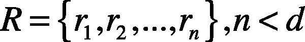
Assuming F = {f1, f2, …, fd} is a d-dimensional feature space, feature selection means to delete some features from the original d-dimensional feature space, and a new feature space R is obtained. Because R is a subset of F, each element ri of R has a corresponding element fi of F, ri = fi. In the process of classifier design, the feature choice is very important to describe an object. Feature selection gives up some features which have little contribution to classification meanwhile some features which can reflect the classification essence are kept.
2.2Feature extractionAssuming F = {f1, f2, …, fd} is a d-dimensional feature space, feature extraction means to extract some of features from the original d-dimensional feature space. The samples of the new concise feature space R is described by n features.
Feature extraction is to find a mapping relationship M.
The above mapping relationship should make the dimension small than the original dimension (Bag & Sanyal, 2011). Every component ri of R is a function of the components of the original feature vector.
2.3Iterative threshold segmentation
The traditional iterative threshold segmentation algorithm (Martinez, Lindner, & Scheper, 2011; Li & Kim, 2010) is based on the approximation thinking. Firstly, an initial threshold value S0 should be select as the follow.
where gmax and gmin are the maximum gray value and the minimum gray value of the image respectively. Secondly, the image is segmented to the foreground area R1 and the background area R2 according to S0. Thirdly, calculate the new segmentation threshold S1.
where g1 is the mean gray value of the area R1 and g2 is the mean gray value of the area R2.
Then iterate the segmentation and calculation of the new segmentation threshold S1 until g1 and g2 do not vary again. Finally, the stable threshold Ss is obtained by the final threshold S1.
After the segmentation, the original gray value p(x, y) becomes p1(x, y).
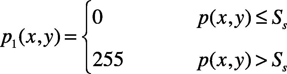
where Ss is the final and stable threshold value of the segmentation.
3NSRA using ITS and GAR techniquesThere are several stages used to complete the NSRA. The flow chart is shown in Figure 1. Firstly, image preprocessing stage is used to filter out the noise and improve the image processing accuracy. Then, ITS is used to obtain the optimal parameters of the foreground and the background, and it will be favorable for the feature extraction. In addition, opening and closing operations are taken to the foreground of image for removing other regions linked to the borderline and the other small targets.

The areas of the foreground of the image would be different between the normal state and the abnormal state. Therefore, the change of the area represents the most important feature of the foreground of an image. In other words, the area of the foreground is the typical feature r1 of the foreground. On the other hand, the cross section of the foreground of the cut section would be different from the normal one. The ratio of the foreground area to the whole cut section would be changed too. So the ratio of foreground area to the cross section area of the cut section was taken as the second feature r2 for the classification.
Successively, the GAR feature vector extraction stage was used to get the two kinds of features of the image. The target of our scheme is to classify the image into the normal state or the abnormal state, thus the classifier structure design is important. Finally, the decision rule is used to distinguish to which classes the unknown pattern belongs. The details of the processing is described below.
3.1Improved threshold segmentation (ITS)Different from the traditional iterative threshold segmentation algorithm, the ITS algorithm is proposed. The specific steps of ITS algorithm are described as follows.
1. Detect the edge Mi1 of the i-th original image Mi by using Sobel operator templates in 8 directions. Hj(x, y) is the detection result by using the j-th Sobel operator template, j=1,2,…,8. Gmax is the new gray value of the central point of the region 3×3 of image Mi1. Meanwhile, the direction of Gmax is the edge direction of the central point of the region.
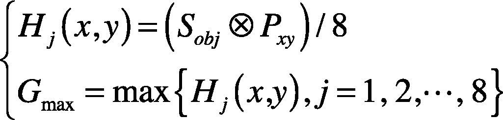
where Sobj is the j-th Sobel operator template, Pxy is a region of 3×3 whose central point is inspected.
2. Set the initial threshold value S0.

where n is the total number of pixels of Mi1. Gmaxk is the gray value of the k-th point of image Mi1.
3. Segment the original image Mi based on S0 to obtain image Mi2 with the foreground and the background, and then calculate the average gray scale values GF and GB of the foreground and the background respectively.
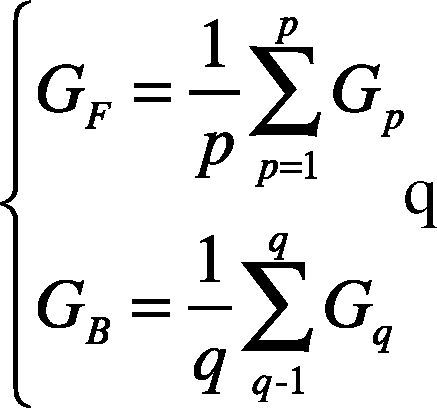
where p and q are the numbers of pixels of the foreground and the background respectively, and Gp and Gq are the gray value of the pixels in the foreground and background in the original image respectively.
4. Calculate respectively the proportion coefficients cf and cb of the foreground part and the background part to the whole image, then calculate the new threshold value S1.
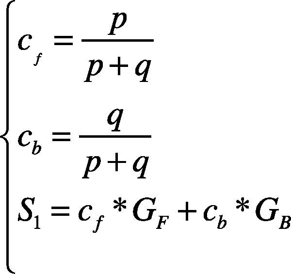
where p and q are the numbers of pixels of the foreground and the background respectively, and GF and GB are the the average gray scale values of the foreground and the background respectively.
5. Judge whether the final threshold Sf is obtained according to the follow rule:
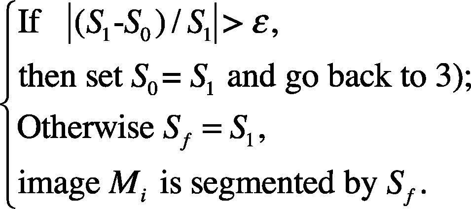
where ¿ is the critical value and Sf is the final threshold value to segment the i-th original image Mi.
3.2Geometric area ratio (GAR) feature vector extractionTo obtain the features of the foreground, the two areas of the foreground and the cross section of cut section should be calculated. But the actual area of the foreground is different from the area in the medical image. There is a proportional relationship between the two areas.
For the same foreground image, the actual area of the cross section of the cut section is different from the area. There is also a proportional relationship between the two areas.
Usually, the same imaging device produces the images with the same specification. This means that the pixel numbers are same. For the simplification, the actual area which is in human body is a, and the corresponding image pixel number which is in the image is n. Then the geometric features r1 and r2 of an image could be constituted. The first feature r1 is:
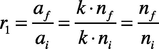
where af is the actual area of the target which corresponds to the foreground part in the image; ai is the actual area which corresponds to the whole image; k is the ratio coefficient of the actual area of the target to the corresponding pixel number in the image; nf is the pixel number of the foreground and ni is the pixel number of the whole image.
The second feature r2 is:
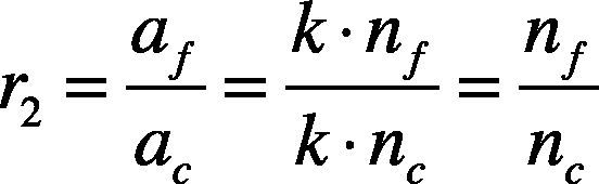
where ac is the actual area of the cross section of the cut section of the target, and nc is the pixel number of the cross section of cut section.
There are the relationships below:
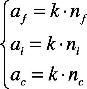
The two features built by equations (12) and (13) are both the geometric area features of the foreground of an image.
The feature extraction flow chart using GAR is illustrated in Figure 2. It can be seen from Figure 2 that GAR feature extraction needs five steps and four transient images of Mi1, Mi2, Mi3 and Mi3 should be produced during the feature extraction process from the original image Mi. Then, GAR feature vector can be extracted by the calculations. The feature extraction method of GAR is described as the five following steps:

Step 1. Preprocess the i-th original image Mi by sharpening the image with Laplacian operation lp(x, y) and taking the filtering with the median filtering operation mf (x,y).
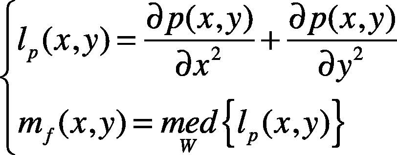
where p(x,y) is the original gray value of the image, and W is the window.
The first transient image Mi1 was obtained from the original image Mi.
Step 2. To obtain image Mi2 with the clearer borderline, the image Mi1 is segmented by using ITS which was described in section 3.1.
Step 3. For removing the other regions which are linked to the borderline and the other small targets, the opening operation and closing operation are taken to produce image Mi3 and Mi4.
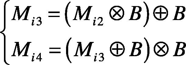
where B is the structural element.
Step 4. Calculate the two features of the image foreground to constitute the 2-dimensional feature vector Ri of the i-th sample image.
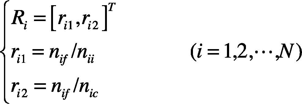
where, nif is the pixel number of the foreground of the i-th sample image; nii is the pixel number of the i-th sample image, and nic is the pixel number of the cross section of the cut section of the i-th sample image.
Step 5. Judge whether or not the N feature vectors are completed.
3.3Decision rule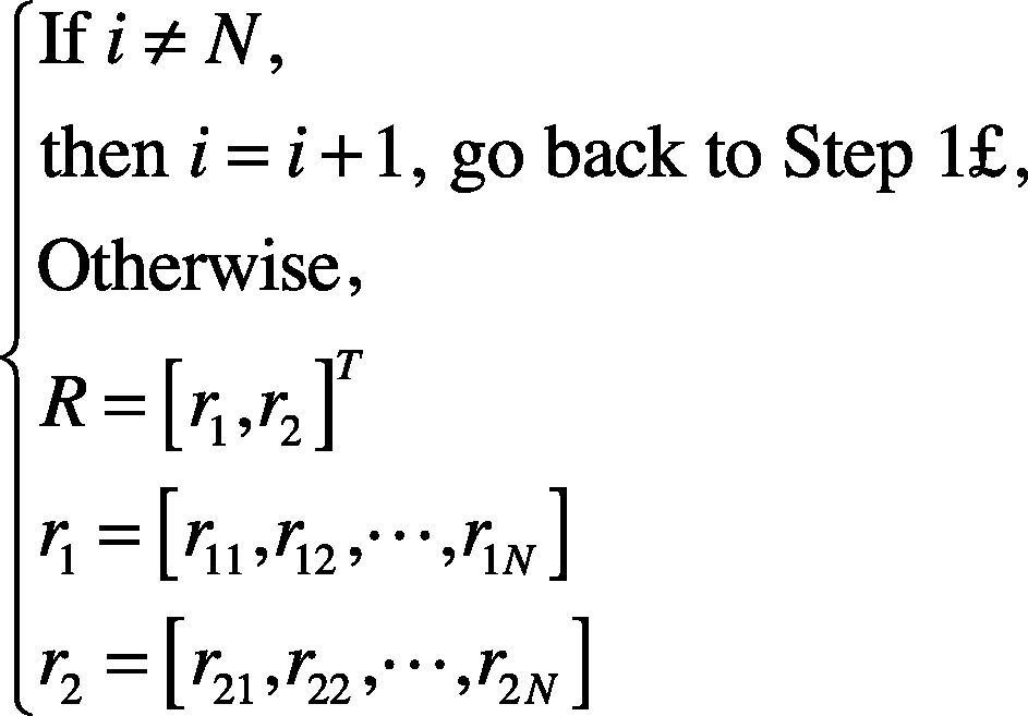
The classifier design involves the metrics to measure the similarities and the distances. It also involves the decision rule.
Before the classifier is designed, we would like to give the decision rule, the definition of a distance from a point to a cluster of GAR and the metric of GAR method.
3.3.1Definition of distance from a point to a clusterIn order to design the classifier, the distance dRCi from a feature vector R to a cluster Ci is defined as follows:
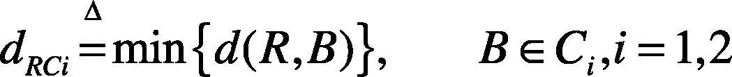
where Ci is a cluster, B is any element of cluster Ci, and dRCi is the Euclidian distance between a feature vector R and feature vector B.
Assuming that Ri = [ri1, ri2]T is a feature vector or a pattern and Rj= [rj1, rj2]T is another pattern, then the Euclidean distance dRiRj between the two patterns is as below:
3.3.2Definition of decision rule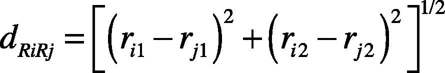
We define the decision rule as follow:
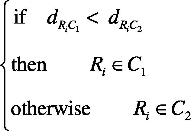
where C1 and C2 are two clusters, and Ri is an unknown pattern to be recognized.
3.4Classifier structure designThe classifier structure is designed in Figure 3. In the figure, Ri is the input feature vector which belongs to class C1 or class C2; dRC1 and dRC2 are the distances from the unknown pattern R to the cluster C1 and C2 respectively. It can be seen that R is decided to the class which has the minimum distance to the the unknown pattern; dRC1 and dRC2 can be calculated according to equation 19.
3.5Two cluster models generation
For the classification method, more and more types appeared with the developments of science and technology, such as the classical statistical classification, cluster computing (Salukvadze, Gogsadze, & Jibladze, 2012), structure recognition, and neural networks. In this paper, K-nearest neighbor clustering would be used for the generation of two cluster models.
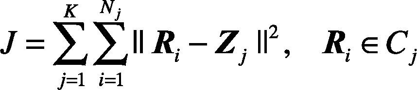
K-nearest neighbor clustering method (Gao et al., 2009) is based on the minimization of the criterion function. The criterion function is defined as the sum of the squares of the distances between each sample Ri to the corresponding cluster center. For the j-th cluster, the criterion function Jj is defined as below:
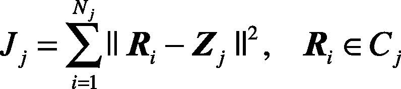
where Cj is the j-th cluster and its central point is Zj. Nj is the sample number of the j-th cluster Cj.
For the K clusters, there is
According to the clustering criterion, cluster centers should be chosen so that the criterion function J takes the minimum value. That is to make Jj minimal. Then there is
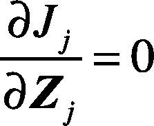
It can be rewritten as follows:
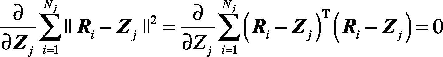
The result is obtained:
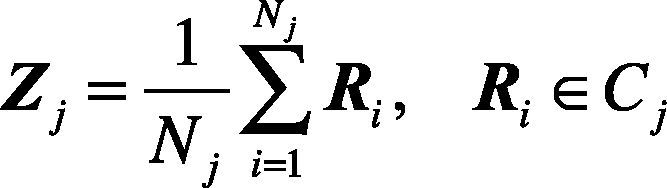
It is shown by the above equation that the center of the cluster Zj is the mean value of the samples of the clustering Cj.
K-nearest neighbor clustering method (Connor & Kumar, 2010) is described below.
Select the initial number K of cluster centers and the initial centers Z1(1), Z2(1), …, ZK(1). The number in the brackets is the sequence number of the iterative calculation.
Assign the remaining samples to one of the K clustering centers according to the minimum distance rule.
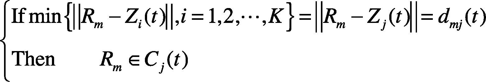
where Rm is a remained sample, m = 1, 2, …, N-K; N is the total number of samples; t is the iterative sequence number; K is the number of cluster centers, and dmj is the Euclidian distance between the point Rm and the point Zj(t).
3. Calculate the new vectors of the cluster centers.
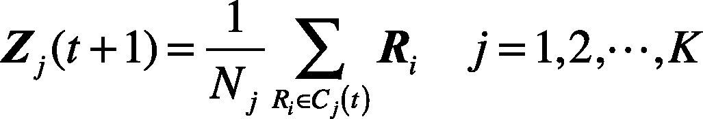
where Nj is the sample number of the clustering Cj.4. If Zj(t+1)≠Zj(t) j=1, 2···, K, go back to 2; otherwise, Zj(t+1)=Zj(t) j=1, 2, ···, K..
3.6Novel state decision rule (NSDR)The NSDR of the GAR algorithm is described below:
Step 1. Set i = 1.
Step 2. Input image Mi and preprocessing it to obtain Mi1.
Step 3. Segmented Mi1 with the optimal threshold S:
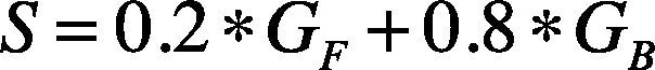
where GF and GB are the average gray scale value of the foreground and the background, respectively, and they can be found in equation (9).
In equation (29), the parameters are selected to be 0.2 and 0.8. This is based on the experiments which can be found in Figure 5. It is experimental proved that the edge effect is best when the parameters are selected to be 0.2 and 0.8.
The original image Mi1 becomes Mi2 after the segmentation.
Step 4. To remove the other regions linked to the borderline and the other small targets, the opening and closing operations are taken to the foreground of image Mi2. Mi3 is the image after the opening operation, and Mi4 is the image after the closing operation.
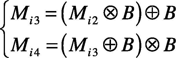
where B is the structural element.
Step 4. Calculate the 2-dimensional vector R of the i-th image feature vector. The calculation formula is in equation (17).
Step 5. If i=N, then go to Step 2; otherwise, fulfill all the N feature vectors of equation (18).
Step 6. Generate the cluster C1 and C2 by using the K-nearest neighbor method above.
Step 7. Classify the unknown sample according to the decision rule in equation (21).
Step 8. Output the results states.
In NSDR, the different class is used to represent the different state of the foreground of the image.
4Experiment and analysisIn order to demonstrate the effect and correctness of NSDR, some medical images with 512×512 pixels were selected as the experimental objects. All the results were obtained by using software MATLAB R2011a.
4.1Experiment environmentThere are some thyroid images with the size of 6×5 cm2 and they are in the normal state or the abnormal state. For every thyroid image, the finally experimental feature vector is obtained by GAR method. These data are divided to the training data and the test data. The classifier is trained and tested respectively by the training data and the test data.
Figure 4 shows the thyroid computerized tomography (CT) images. The two leaves of a thyroid surround the circular part in the upper parts of Figure 4. Due to the small and thin volume, the thyroid is invisible and intangible in the neck in the normal case. If the thyroid cannot be seen but can be touched in the neck, it often is considered that the swollen thyroid occurred. This kind of intumescence is generally physiological enlargement, especially in female puberty; but it is sometimes an ill enlargement. The CT images of the normal thyroid and abnormal thyroid are respectively shown in Figures 4A and B. It can be seen that the two leaves part of the abnormal thyroid is obviously swelling in the Figure 4B.
4.2Experiment result thyroid images. A: normal thyroid CT image. B: abnormal thyroid CT image.")
The ITM is used to obtain the optimal parameter for the thyroid image segmentation. The edge effects of the ITM are shown in Figure 5.
 of the abnormal thyroid image. A: original image. B: traditional threshold segmentation. C: ITS with cf = 0.1 & cb = 0.9. D: ITS with cf = 0.2 & cb = 0.8. E: ITS with cf = 0.3 & cb = 0.7. F: ITS with cf = 0.4 & cb = 0.6. G: ITS with cf = 0.5 & cb = 0.5. H: ITS with cf = 0.6 & cb = 0.4. I: ITS with cf = 0.7 & cb = 0.3. J: ITS with cf = 0.8 & cb = 0.2.")
Edge effect of improved threshold segmentation (ITS) of the abnormal thyroid image. A: original image. B: traditional threshold segmentation. C: ITS with cf = 0.1 & cb = 0.9. D: ITS with cf = 0.2 & cb = 0.8. E: ITS with cf = 0.3 & cb = 0.7. F: ITS with cf = 0.4 & cb = 0.6. G: ITS with cf = 0.5 & cb = 0.5. H: ITS with cf = 0.6 & cb = 0.4. I: ITS with cf = 0.7 & cb = 0.3. J: ITS with cf = 0.8 & cb = 0.2.
Figure 5A is the original image of an abnormal thyroid. It can be seen the right leaf is bigger than the left leaf and the two leaves are not balanced. Figure 5B is the edge of traditional threshold segmentation (TTS). Figures 5C-J are the edges of the ITM with different parameters cf and cb.
It can be seen from Figure 5 that the proportions taken by the foreground become small and small when the parameter cf increases. Especially, the oversegmentation results become more and more serious when the parameter cf is more than 0.3.
Compare the edge results of Figure 5C to Figure 5J, cf = 0.2 and cb = 0.8 are the optimal parameters of the ITS in Figure 5D; compare Figures 5B and D, the better edge is in Figure 5D because it has the clearer thyroid edge and it is more suitable for calculating the GAR feature vector.
The partial feature extraction processes of the two leaves of the abnormal thyroids are given in Figure 6. It can be seen that the two leaves of the thyroids are asymmetrical and irregular because they were in the abnormal state.

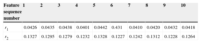
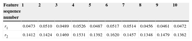
Table 1 shows the GAR feature data of the normal thyroids, and Table 2 shows the GAR feature data of the abnormal thyroid.
We can find that the first feature range of the normal state thyroids is from 0.0401 to 0.0442 and the second feature range of the normal state thyroids is from 0.1227 to 0.1328; meanwhile the first feature range of the abnormal state thyroids is from 0.0456 to 0.0526 and the second feature range of the abnormal state thyroids is from 0.1348 to 0.1479. The feature vectors of different classes are distributed in different regions.
Figure 7 is the recognition results of NSRA method. In Figure 7, the symbols of green and blue ‘*’ represent respectively the normal and the abnormal training sample points. The symbols of red and magenta ‘•’ represent respectively the normal and the abnormal test sample points. r1 and r2 represent respectively the two features of the GAR of the thyroid. In Figure 7, r1 is 10 times of the ratio of the thyroid area to the whole image area, and r2 is the ratio of the thyroid leaves area to the area of the cross-section of the cut-section of the thyroid.

Figure 7 shows the results of NSRA method: 1) the proposed GAR feature vectors can reflect effectively the similarities of the samples in same classes of the normal and abnormal states of thyroids; simultaneously, the vectors can distinguish the distances of the different classes; 2) the presented NSRA of the designed classifier is suitable for the state recognition of thyroids.
The experiment result demonstrates NSRA was correct and effective. It can achieve the correct classification for the unknown test samples.
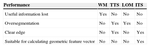
4.3Performance comparisonTo demonstrate the effect of GAR method, the edge comparison was given in Figure 8.

Figure 8A is the edge effect of Wavelet method (WM) on 1st level; Figure 8B is the edge effect of TTS; the edge effect of LOM was given in Figure 8C; Figure 8D is the edge effect of ITS. Compare Figures 8A, B, C and D: too much information was lost in Figure 8A; the oversegmentation appeared in Figure 8B and the seriously oversegmentation occurred in Figure 8C; the clear edge appeared in Figure 8D, which was the best result for calculating the GAR feature vector.
The performance comparison of different method was shown in Table 3, from which it can be seen that the ITS has the best result for the feature extraction of GAR method.
ConclusionsIn this paper, we proposed the NSRA for the target state recognition. To extract the novel feature vector of GAR, the ITS is developed to acquire the optimal parameter with the clear foreground edge of the medical image; to design the classifier, the distance between a pattern and a cluster is defined, and then NSRA is presented; to demonstrate the correctness and the effect of NSRA, the experiments were implemented and the comparison was made. Experiments show that the GAR feature vector can effectively reflect the similarity of the same class and the difference between the different classes of thyroid states. Furthermore, the NSRA can recognize the normal state and the abnormal state. In a certain extent, the study of this paper achieves the computer-aided decision of the normal state and the abnormal state of a target in an image.
This research was sponsored by Scientific Research Foundation for Returned Scholars, Ministry of Education of China ([2011]508), and Natural Science Foundation of Shaanxi Province of China (2011JM8005), and the National Science Council, Taiwan (R.O.C.) under contract NSC 101-2221-E-167-034-MY2.