


It has been shown that, at least in simulated scenarios of variability decomposition in size and frequency, the way these components are measured largely determines the shape of their relationships. This study aims to build on this specific finding and tests how these measures of variability components behave on real data. Moreover, getting advantage of the type of available data, several models are setup to assess amplification on such variability components, and to evaluate the impact of the product type on both: amplification and component variability behaviors. We do this by performing model assessment with the traditional un-weighted C.V. measure, and then replicating the same evaluation with the recently proposed ADV measure.
Se ha demostrado que, al menos en escenarios simulados de descomposición de variabilidad, en tamaño y frecuencia, la manera en que se miden estos componentes determina en gran medida la forma de sus relaciones. Este estudio tiene como objetivo construir en este descubrimiento específico y evalúa cómo estas medidas de los componentes de variabilidad se comportan con datos reales. Además, aprovechando el tipo de información disponible, varios modelos son configurados para evaluar amplificación en dichos componentes de variabilidad, y analizar el impacto del tipo de producto en la amplificación y los comportamientos de variabilidad de los mencionados componentes. Hacemos esto mediante análisis de modelos utilizando la medida tradicional C.V. no-ponderado, y luego replicar la misma evaluación con la medida ADV propuesta recientemente.
There is no question that variability is omnipresent and ubiquitous in most operations. However the way it manifests is not always the same, and this is especially true for demand variability, which in our case is the demand issued by the immediate lower echelon or in other words: order variability. This order or demand variability is a major issue for all industries since the planning of assets, infrastructure and operational resources is affected by flows regularity or, in better words: flows variability. For example Cedillo and Ramírez [1] proposed a dynamic self-assessment method for supply chain performance, they conclude that inventory of finished goods and work in process are two of the most important factors determining SC performance. They directly and indirectly linked these factors to order variability as depicted in its casual loop diagram. Additionally, knowing the types of variability manifestations (i.e. components) along with the relationships among these components, and in turn, its impacts on operations can help cope with the unwanted effects of this phenomenon. However, there are still some further issues: variability is a hidden entity; we do not really see it but rather perceive it through its effects. The way we usually depict it is through measuring and, it is a fact that there are several measures to capture it. The latter is not a minor issue in any area of science. For instance, Rodríguez et al. [2] deal with Heart Rate Variability (HRV) in medical science, they state “…the human cardiovascular system is characterized by a high degree of complex variability, such that many standard measures obtained from HRV can lead to incorrect conclusions and dangerous extrapolations”. They even go further and suggest that some methods such as statistical physics or nonlinear analysis “… might provide important insights for physiological interpretation of HRV and for the assessment of the risk of sudden death”. Hence, which variability measure is the most appropriate for a specific case? Is there a single overall generic measure suitable for all? Do variability components behave constantly through different measures? Does the specific measure matters for decision making?
The above are the questions that this study aims to address, and their importance to an organization's costs, service level and overall planning process is quite obvious for any operational sensitive mind. Moreover, there are some industries where variability decomposition is highly critical as explained by Inderfurth and Mukherjee [3], in the spare part provision operations; where they claim that “…it is not only the uncertainty, but also the time-variability of demand and return level that makes efficient spare part acquisition during Post Life Cycle a rather complex problem”.
The main contribution of this study is the assessment on real data, of the idea that the type of variability measure matters in decision making; comparing a new proposed, and from our point of view “more suitable” for our case, variability measure, versus a commonly utilized and widely accepted measure such as the classical un-weighted CV. The latter provides not less important insights on the relationships among the variability components and their behaviors with different data sets, such as product categories and echelon position in the supply chain. It is important to note and to stress the point that our contribution is not on magnitude decomposition of time and size, rather than on the variability decomposition of time and size. The first is a classical decomposition in literature while the latter is not yet fully addressed to say the least. We will elaborate further in the following sections.
2BackgoundEvidently, daily demand can only vary on two dimensions: order size, and whether that order was placed or not each consecutive day i.e. time. In addition, variation of order quantity and order frequency can be related to each other. This is also intuitive since at lower echelons usually the objective is to fulfill a specific demand volume within a specific time period through the placement of orders. Then, the total amount ordered and distributed throughout the period has to eventually meet the overall demand quantity. Thus, a negative correlation between order quantity and frequency can be expected.

Customers (i.e., lower echelons) and products may have different attributes that affect daily demand, and thus, its variation. A customer, for example, might decide to purchase fixed order sizes (given transportation or receiving dock restrictions), in which case daily variance might manifest itself through a variance in the frequency of ordering rather than a variance in the order quantity itself. The way these different variability components behave, may influence in turn, different corresponding operational decisions at the upper echelon. Therefore, each of these decision processes could be benefit from knowing, not only the overall variation, but also the type of its variation components.
Under the previous considerations, we can formulate the following hypotheses:
H1: Frequency and volume variation are positively correlated to daily demand variation.
We have mentioned that frequency and volume variation are components of daily demand variation. Therefore, an increase in either one of these components would imply an increase in daily demand.
H2: Order variation and frequency variation are negatively correlated to each other.
This hypothesis is a consequence of assuming that managers have in mind a daily overall demand target that they are trying to meet. If this assumption is correct, then for a given demand pattern, if order frequency become steadier (e.g. from variable to fixed or negative variability), then order size would have to adapt to respond to demand changes (e.g. from fixed to variable or positive variability). This idea was discussed by Bivin [4] in a production environment, where he stated that the size of production lots is inversely related to the frequency of production. However, this hypothesis depends on the inventory policy that clients placing the order are using.
H3a: The number of echelons downstream of the client is positively correlated to all three types of variations
H3b: The number of echelons downstream of the client is negatively correlated to all three types of variation.
As we discussed before, the number of echelons refers to the number of clients' layers downstream the orders' placer. Since Distribution Centers sell to retailers or other wholesalers (instead of selling to final consumers), they are assumed to have a larger number of downstream layers than retailers who sell directly to final consumers. Hypothesis 3a comes from the idea that variation is amplified as one move upstream in a supply chain, a phenomena called “bullwhip effect” (as in Lee, Padmanabhan, and Whang [5]). Experimental settings using the beer game also find amplification of variability from downstream to upstream players in a supply chain. See, for example, Sterman [6], Croson and Donohue [7] and Croson, Donohue, Katok, and Sterman [8].
Hypothesis 3b assumes that D.C.s can implement some “scheduled ordering policy” with their retailers (for example, as in Cachon [9]). Blinder [10] showed a smaller variance of the trend of retail sales than the variance of deliveries to retailers. Of course, just as in the case of hypothesis 2, the actual effect of adding more echelons or of having certain echelons that aggregate demand across many firms in a supply chain depends on the inventory policy that each echelon/firm is using -see, for example, Caplin [11] who shows that if firms use an (s,S) policy, the effect should still be present after aggregation, and Baganha and Cohen [12]. Although Schmidt, Cachon and Randall [13] do not find an amplification effect at the industry level when comparing non-seasonally adjusted manufacturing and wholesale sales, they do find amplification between retailers' and wholesaler's sales. Similar results are noted in Baganha and Cohen [12]. Blinder [10] and Blinder, Lovell and Summers [14] also finds amplification between retailers and wholesalers. Chatfield, Kim, Harrison and Hayya [15] find that information sharing reduces variance amplification in a k-stage serial supply chain simulation model. Since the echelons that we have in our database are downstream of a manufacturer of end products, then these papers would support hypothesis 3b (since our database includes manufacturer sales to retailers and to D.C.s,i.e., wholesalers, the former would be equivalent to “wholesaler sales” and the latter to “manufacturer sales”). However, it is important to note that the above mentioned papers study variance at the industry level, while our hypotheses are at the sku-destination pair level. While different levels of aggregation will be discussed and tested later in this paper, this papers studies variability an individual firm level.
The idea of testing both, Hypotheses 3a and b, under different variability measures is supported by some studies that clearly state the different forms in which the bullwhip effect is being measured. One example is Warburton [16], who analytically investigates variability amplification using different Bullwhip Effect measures.
H4: Product Category is significantly correlated to all three types of variations.
We have stated that product characteristics could have a significant impact in operations. Product features such as obsolescence risk, size, price, or sales volume may directly affect inventory levels or production runs, and thus, variation of order size, frequency and daily demand. This relation between product attributes and operations is deeply explored by Kleijnen, and Smits. [17], who explore metrics for supply chain management that are closely related to product attributes. Product categories tend to be formed by products sharing common characteristics, therefore testing the impact of product category on variation is a way to test sets of products with similar characteristics against other product sets with different features.
H5: Product Category is significantly correlated to amplification in all three types of variation.
In hypothesis 3a and 3b we discuss the potential impact of the number of echelons on variation (i.e. amplification). However, there could be certain variation amplification behavior due to product characteristics. For example, suppose a product has very low average sales volume as compare to full truck loads. Then, even though D.C.' downstream clients would, in this case, not order enough to fulfill a truck load, the D.C.'s will tend to carry inventory and order to the manufacturer in full truck loads (i.e. batch orders as in Lee, Padmanabhan, and Whang, [5]), which would produce amplification. At the same time, a product whose average volume was enough for a full truck load would not exhibit amplification. Similarly, some product categories might be subject to more frequent price promotions than others, creating a rationing game (as in Lee, Padmanabhan, and Whang, [5]). Therefore, product characteristics can affect the degree of amplification.
In order to test these hypotheses, we used order and shipment information from a confectionery manufacturer. This information contained and distinguished different types of clients and different product categories which we believe, as stated before, influence the variability of order patterns. We present a set of models that would help us determine how strong and significant, if at all, are the relations of these variables and their attributes to the different types of ordering behavior we already discussed.
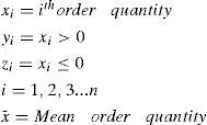
For each “SKU-Ship to” (SS_pair) in the sample, we calculated the average and the standard deviation of the following variables:
- •
Daily Demand;
- •
Ordered Quantity;
- •
Interval (days between the current order and the previous order for that SS pair).
To standardize these metrics, and make variance comparable across different magnitudes, the coefficient of variation (CV) was proposed as an inequality index for each of the metrics defined above. The coefficient of variation is a scaled measure known to be dimensionless, which allows for cross item comparisons. However, there are two possible formulas to calculate the CV (Sheret [18]). One of the formulae takes into consideration weights for the distribution of the resource, which in our case are orders. The other option for CV calculation is the traditional formulae being the division of the standard deviation over the mean, which does not consider weights.
The structure of our data distributes the weights evenly and consistently within our unit of analysis: SS_Pair. Moreover, the fact that we are grouping orders of the same SS_Pair with the same required delivery date assures the same weight for each observation. So, in our case traditional unweighted CV calculation is sufficient as an inequality index.
We have developed some models that would help us test hypothesis 1 through 6, using the latter unit of analysis and the standardize metric.
Notation:DD = Daily demand coefficient of variation Frequency coefficient of variation Volume coefficient of variation dummy variable for product category dummy variable for type of client index of dummy for product category I, I ϵ (1,2,3) index for dummy type of client j, j ϵ (1,2) Number of product categories=3 (S,F,P) Number of type of clients=2 (D.C., Retailer)
H1: Frequency and volume variation are positively correlated to daily demand variation.
Model 2
H2: Order variation and frequency variation are negatively correlated to each other
Model 3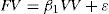
H3a: The number of echelons downstream of the client is positively correlated to all three types of variations
H3b: The number of echelons downstream of the client is negatively correlated to all three types of variation.
H4: Product Category is significantly correlated to all three types of variations
H5: Product Category is significantly correlated to amplification in all three types of variation:
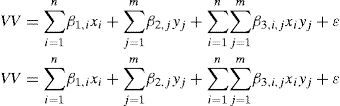
The first term in all equations in model three, will test the effect of product category on the coefficient of variation for its corresponding type of variation. The second term will account for the impact of the type of client (which is a proxy for the number of echelons downstream of the firm), while the third term will consider the interaction of product category with the type of client.
3MethodWe devise two possible methods to follow in order to obtain the estimates for the proposed models. Generalized Linear Models (GLM) or Ordinary Least Squares (OLS). GLM does not require identifying the proper distribution of the data, however, for a more powerful regression this is advisable prior applying GLM directly to obtain the effects of the corresponding models. Afterwards, we would need to avoid the bias in the variance-covariance matrix in order to correct for heteroskedasticity, we do this by calling for an unbiased variance-covariance matrix in STATA. STATA GLM assumes a distributional form for the variance covariance matrix, which of course, is not the variance times the identity matrix, (i.e. no constant conditional variance across X).
For our data the most likely candidate is the Gamma Distribution. We will choose then to run GLM under the assumption of Gamma distribution and correct for heteroskedasticity to evaluate the proposed models.
4Analysis and resultsWe begin the analysis of hypothesis 1. However, prior to run the generalized linear model, we need to identify the link function. GLM assumes that the dependent variable is a function of a linear combination of the independent variables. That function is called a link function and can take different forms depending on the nature of the relationship between dependent and independent variables. We believe that the effect of frequency and order size coefficients of variation on daily demand variation is additive; this is derived by the intuition that lumped orders would be represented as an arithmetic sum in daily demand, and not as a factor. Nevertheless, we have chosen to run GLM using additive, multiplicative and canonical link function to evaluate the proposed models.
Results from the deviance, AIC and BIC show that gamma with additive function does a better job explaining the relation. They indicate that both coefficients are significant and positive, suggesting a positive relationship with daily demand variation; which supports hypothesis 1.
For the second hypothesis Gamma canonical prompted no results due to unfeasibility of the initial values. Results from the additive model prompted values for deviance and AIC far too high to be a good option explaining the effect of vv on fv. Multiplicative yields a good fit according to AIC with an acceptable deviance. This last model suggests a negative relationship between VV and FV, so hypothesis 2 holds.
We look now to test hypotheses three (a,b), four and five. All three link functions prompted the same values for AIC, BIC and Deviance, as well as for the log likelihood, which in this case being negative was indicating a loss function minimization. The relevant values indicate a good fit; in all three models, F-distribution center interaction dummy is dropped together with the interactions of S-D.C., F-Retailer, and P-Retailer, due to multicollinearity. In addition, the model for the frequency coefficient of variation (FV) drops the F dummy while the remaining two models with volume and daily demand coefficients of variation drop the D.C. dummy.
Observing the results from the FV model, we notice there are only four significant variables: S, P, Retailer and D.C., all of them are positive suggesting a positive relationship with frequency variation. In more detail, the coefficient of D.C. is larger than the coefficient of retailer suggesting a larger variability when the number of echelons downstream increases. However, std. error for D.C. is larger than standard error for retailer and, more importantly, D.C.'s 95% confidence interval is considerably wider than retailer's and includes the value of the retailer's coefficient; therefore, we cannot conclude a difference effect on the type of client, and thus, on the number of echelons. So hypotheses 3a and 3b have no support by these results.
Product Category on the other hand is relevant for all three types of variations, since their estimators are significant and positive; S being more relevant for daily demand and order size variation while P for frequency order variation. Hypothesis four seem to hold under these results.
No interactions were found significant, meaning that no amplification was found due to product category, hypothesis five does not hold.
We can observe from our results that daily demand variation increases as either frequency or volume variation increases. Also, there seems to be a tradeoff between order and frequency variation. The number of levels prior to end demand does not have any impact on any of these variations, so no amplification or dampening was found. Finally, product types have a positive effect on all types of variation.
We now move to perform the hypotheses analysis using the Absolute Differences (From the Central Mean) Variation or ADV measure. As stated in Monsreal et al. (unpublished) [19], this measure features the four main properties sought for a correct assessment of variability components: dimensionless, simple, complementary and consistent.
For convenience, we reproduce the formulae stated in Monsreal et al. (unpublished) Let us define
Then:

When we asses normality and homoskedasticity on the new main variables, we observed that these new variables fail to show normality and homogeneous variance. Then we can conveniently assume a Gamma Distribution. The latter allows using the same method of analysis (GLM) as for the C.V. variables. This would make results more comparable and valid since GLM does not require the identification of the specific data distribution.
Even though AIC and BIC are very similar among all three models, AIC and deviance lean the scale, once again towards the additive function. Based on this function, ADVSize and ADVfreq have a perfect and significant relation with ADVOrders, and thus, results support hypothesis 1.
For hypothesis 2 the Gamma canonical function was feasible. However even though AIC and BIC values are very alike, the deviance favors the additive function, as opposed to the CV assessment. Results show a counterintuitive positive relationship between frequency and size, and therefore do not support hypothesis 2.
We turn now to hypotheses 3a, 3b, 4 and 5. All three link functions show the same vales for AIC, BIC, deviance and log-likelihood for ADVFreq, ADVSize and ADVOrders.
All models retain the same variables (S, P, F, Retailer, P-D.C., and S-Retailer). Out of these variables, all models suggest only 4 to be significant: S, P, F, and P-D.C. Then, we can conclude that hypotheses 3a and 3b do not hold since variables D.C. and Retailer were dropped. Hypothesis 4 has significant support showing a positive relationship for the three types of product for the three types of variability. Finally, hypothesis 5 is partly confirmed by a mild but significant coefficient value exclusively for the interaction of P and Distribution Center. This last value suggests a variability dampening when orders are being issued by a Distribution Center, presumably due to a pooling effect.
5Conclusions and further researchWe have assessed a series of hypotheses under two different variability measures on real data. Hypotheses were focused on determine variability components behavior, amplification and the influences of type of product on both. Results vary from one measure to the other. However both measures confirm a positive relation between each variability component and daily demand or order variability. Also, they suggest no amplification effect due to the number of echelons, and found a relevant role of the type of product on the behavior of the variability components. Main differences between the two types of measures lie on the relation between order and frequency variation. While C.V. suggests an inverse behavior, ADV measures finds a positive relationship. Explanations for this can be drawn from two different perspectives: If we take into consideration the initial thought that variability should be split among the two components to meet a specific demand, then C.V. results seem to be more adequate. However, it was not uncommon for clients to do some kind of gaming. At times they'd order more than the real demand and expect the manufacturer to take it back if it remained unsold, especially for promotional item. The latter would largely explain the positive correlation supported by the ADV measure; unfortunately not all of these types of orders are explicitly identifiable in the data. Additionally, notice that hypothesis 1 is confirmed by both measures, based on this if the overall variability increases then both variability components would tend to increase, overriding (i.e. contradicting) hypothesis 2. Further exploration on this specific hypothesis is needed. The last difference between both measures is on hypothesis 5, C.V. showing no support while ADV finds a dampening effect for the case of a type of product (P) going through a Distribution Center. The main finding of this study is confirming, on real data, that the type of measure used to determine variability, at least in its decomposition of time and size, matters. However, further assessment is needed considering other type of scenarios, which could include aggregated scenarios by product or client.
The authors wish to thank Professor Björn Claes for providing access to, and useful insights of, the data set.