


Monitoring of water sources is a major concern worldwide. Wireless sensor networks (WSN) may be used for this monitoring. However, current systems employ mainly physical sensors for variables such as temperature, pressure, humidity and light. Wireless chemical sensors networks (WCSNs) for environmental monitoring are scarce due to the lack of autonomy of conventional sensors. This paper presents results of a WCSN for monitoring pH based on ion selective field effect transistors (ISFETs). Sensing nodes employ a human interface required for in situ calibration of chemical sensors. Unlike most studies, our work evaluates the network employing chemical measurements and wireless network metrics. Results show zero packet losses by using a time division multiple access (TDMA) protocol. The network allows wireless communication within 300m including attenuation from buildings and trees. Therefore, the system presented in this paper is suitable for long range applications with unobstructed line of sight. pH measurements present a standard deviation below 1%, showing high repeatability. When compared to a commercial pH meter, difference in measurements is below 5%. As a consequence, accuracy is adequate for the application. Measurements also presented high stability during 3h of continuous measurement.
Water quality is a major concern worldwide due to increased demand and pollution. Regulations such as The Clean Water Act (United States Congress, 1972) in the United States and The Water Framework Directive (European Parliament, 2000) in Europe, provide guidelines for monitoring aquatic environments. There are different parameters related to water quality, such as pH, dissolved oxygen and electrical conductivity (Ding, Cai, Sun, & Chen, 2014). Sensor technology is rapidly evolving and these parameters can already be measured in field. However, most water analyses are carried out in centralized laboratories based on the application of conventional monitoring techniques to field-collected samples.
Recent advances in micro-nano-systems, microprocessors and low-power radio technologies have created low-cost, low-power, miniature sensor devices. The devices can be connected to form a wireless sensor network (WSN) (Chong & Kumar, 2003), a key enabling technology to observe changes in physical phenomena. The technology is likely to replace portable instrumentation and data-logging devices requiring a wired connection. These devices provide real-time interaction of monitoring systems, especially in remote areas. WSNs have been already proposed for applications related to wastewater, surface water and pipeline monitoring and represent a formidable candidate for fulfilling the requirements of those applications (Hart & Martinez, 2006).
Currently, the practical application of WSN to chemical analysis for environmental monitoring is scarce (Bonastre, Capella, Ors, & Peris, 2012). Main examples employ physical sensors, such as temperature, pressure, humidity and light sensors (Crowley, Frisby, Murphy, Roantree, & Diamond, 2005; Martinez, Hart, & Ong, 2004). However, the use of chemical sensors for in field measurements is challenging due to the inherent difficulties associated with measuring chemical parameters in liquids for long periods of time and without sensor maintenance. Main difficulties are sensor autonomy, durability and response variability due to temperature and other external factors. Therefore, the use of ISFET based sensors is promising, since they exhibit characteristics such as robustness, miniaturization, seamless integration in microsystems, low power consumption and rapid response.
Additionally, wireless communications may be challenging depending on application and distance between nodes. One example presents a temperature monitoring system for shellfish catches. The system employs 433MHz radios with maximum distance of 10m between transmitter and receiver nodes. However, communication is interrupted when nodes do not have direct line of sight (Crowley et al., 2005). Another example presents a WSN for measuring temperature, humidity, leaf wetness, rain, solar radiation, wind speed and direction. The system uses 868MHz radios with link lenghts up to 7.64km (Mariño, Fontan, Dominguez, & Otero, 2010). Both of these systems employ proprietary communication protocols.
In the other hand, there are several examples of WSNs employing standard communication technologies. Kim, Evans, and Iversen (2008) presented a system for measuring soil electrical conductivity, with radio ranges up to 700m employing Bluetooth. Therefore, maximum number of nodes in the network is seven (Bluetooth-SIG, 2004). Another system employs Zigbee Pro radio modules to send soil moisture and temperature data (Gutierrez, Villa-Medina, Nieto-Garibay, & Porta-Gandara, 2014). However, there is no information on distances covered with the network.
All systems mentioned employ communication protocols with few options (if any) for customization. Additionally, all of them employ physical sensors and do not provide information regarding measurement precision or wireless network packet reception.
Regarding the application of WSN to chemical sensing, a system with optical sensors based on LEDs and polymer coatings has been described for chemical plumes detection (Shepherd, Beirne, Lau, Corcoran, & Diamond, 2007). The study shows 5 nodes within a chamber of maximum 2m wide. Other examples include systems based on voltamperometric silicon microelectrodes for cadmium (Yun et al., 2004) and magnetoelastic pH sensors (Yang et al., 2002), with 3m maximum distance between nodes. Another work describes the use of ion selective electrodes (ISE) for nutrient monitoring (Capella, Bonastre, Ors, & Peris, 2010). This system employs fourteen nodes and results compared with standard techniques are good. However, the study does not mention the distance betwee nodes. None of these papers provide quantitative results regarding wireless network performance.
There are several examples in the literature about the specific monitoring application of pH and other parameters. The study presented in (López, Go¿mez, Sabater, & Herms, 2010) describes pH detection and data transmission using IEEE 802.15.4. However, the study does not include information regarding packet loss or accuracy of pH measurements. Another study describes a wireless sensor system for measuring chlorine, pH and temperature. The network includes repeaters, sensors and main nodes, using the 2.4GHz frequency band (Chung, Chen, & Chen, 2011). However, the paper does not report on network performance variables and accuracy on chemical variable readings. The work presented in (Cheng, Chou, Sun, Hsiung, & Kao, 2012) uses four sensors (pH, K+, Na+ and Cl−) in the same node and Bluetooth communication. The study employs only one sensor node with maximum transmission distance of 10m with 99% reliability. Accuracy in pH readings was 1.3%. The work described in Fay et al. (2011) uses ion selective electrode (ISE) for pH measurements. The network includes one transmitter and one receiver, using amplitude modulation (AM) at 400MHz frequency band. However, AM has an energy efficiency of 33% (Haykin & Moher, 2005), considered very small in wireless communications. pH accuracy in the study is better than 2.6%, but the paper does not report results on the wireless system. To the best of our knowledge, the literature employing Xtend modems is scarce. Modems have been used to test wireless networks with no line of sight links (Berdugo, Buchelly, Calle, & Velez, 2012). The test included a multi-hop network with 86m maximum distance between nodes and 1mW transmit power.
The purpose of this work is to present a wireless sensor network designed for a future pH monitoring system in water environments. Therefore, the system needs to transmit information through long distances, and it must provide a way for in situ sensor calibration. The WCSN includes three Ion Sensitive Field Effect Transistors (ISFETs) (Hayes, Beirne, King-Tong Lau, & Diamond, 2008; Jimenez-Jorquera, Orozco, & Baldi, 2009) devices and employs Xtend radio modems (MaxStream, 2007) to transmit information through long distances. Communication uses Frequency Shift Keying (FSK) in 900MHz frequency band, 1W maximum transmission power, and time division multiple access (TDMA) protocol. Because of the long range communication, all sensing nodes are within range of the sink. This paper presents the results of pH measurement and wireless network performance regarding packet losses and maximum radio range, thus providing information on the actual usability of the application.
2System description2.1System overviewThe system includes three sensing nodes directly transmitting to one sink, forming a star topology. The system also includes a software interface for data visualization. Fig. 1 shows main system components.
2.2Transducers
ISFET sensors were built using conventional microelectronic Aluminum gate NMOS technology (Jimenez-Jorquera et al., 2009). The devices are produced on p-type silicon wafers with boron doping of 1.5×1016cm−3. The chip has a size of 3×3mm2. The drain and source areas are often designed long enough to avoid metal contacts close to the gate area, which is exposed to the solution (Jimenez, Bratov, Abramova, & Baldi, 2006). Fig. 2 shows the final encapsulated chip.

ISFETs require a reference electrode to close the circuit. Initial ISFET tests employed one Ag/AgCl double junction Orion electrode. However, long distance measurements employed a pseudo-reference electrode based on a gold microelectrode with an electrodeposited film of Ag and a film of AgCl formed by chlorinization (Almeida, Andrades Fontes, Jimenez, & Burdallo, 2008).
ISFET response is based on two characteristics: its behavior as an electronic field effect device and the phenomena occurring at limit between the electrolyte and the insulator. Ions in the solution create a gate voltage (VGS) shift and a drain current shift (ID). The current flows between the drain and the source of the transistor. Gate voltage can modulate ID to amplify voltage between drain and source (VDS) (Artigas et al., 2001). This situation is modeled by Eq. (1) (Bergveld, 1986):
where μ¯n is the mobility of electrons at the inversion layer, Cox is the gate insulator capacitance per unit area, W is the width of the channel and L is the length of the same channel.
ISFETs employed in this work have a linear response of 45–54mV/pH in a range of 2–10 pH values. Calibration procedure employs two standard solutions, selecting from 4, 7 and 9 pH values. The process places one ISFET in the first selected pH solution, then washes it with distillated water. Finally, the process inserts the ISFET in a different pH solution. Each node collects voltage signals for each of the two pH values and calculates the slope for a linear fit. After calibration, the node computes any other pH value by measuring the corresponding voltage signal and interpolating with the linear fit parameters.
2.3Sensor nodesWCSN have important differences compared to WSN. One of them is calibration required for chemical sensors. The process is executed with a particular frequency to assure data precision for long term periods. This work established a manual calibration protocol, as a first approach for WCSN implementation. Therefore, each node requires a human interface for an operator to perform calibration procedures and verifications in situ. Each node is implemented according to the sensor node architecture presented in Fig. 3.

Power supply employs a 12V DC, 4A-h battery for the whole node including transducers and the radio. Voltage level for the node is very important since signals generated by ISFETs vary according to 50mV for pH unit. Therefore, voltage levels should be as precise as possible. The node uses a ±5 VDC power supply. ISFETs also require ±0.5 VDC. These values were implemented using a Wilson current mirror and a diode. Additionally, ISFETs are sensitive to electrostatic discharges. In order to avoid damages, the node disconnects all power sources when the ISFET moves from one solution to another during calibration or sample measurements.
The conditioning section in Fig. 3 includes circuits for ISFET biasing with constant current of 100μA as in Valdes-Perezgasga (1990), and for creating a DC-level offset of +1.0V to ISFET output voltage. Fig. 4 shows all conditioning elements required for voltage levels before connection to the Control section.
 shows constant current biasing circuit (Valdes-Perezgasga, 1990). Part (b) provides +1.0V offset to the signal.")
Conditioning section. Part (a) shows constant current biasing circuit (Valdes-Perezgasga, 1990). Part (b) provides +1.0V offset to the signal.
Control section in Fig. 3 uses a Microchip PIC 18F4553 microcontroller, with an embedded 12-bit Analog to Digital Converter (ADC). The microcontroller receives voltage signals according to pH values. These values are transformed to ASCII characters representing pH values that will be transmitted every 10s from each node. The microcontroller also implements the communication protocol, by sending information to the radio through RS232 interface. The communication protocol can be modified by changing microcontroller programming. Therefore, nodes in the WCSN allow for testing different protocols without hardware modification.
Fig. 5 shows human interface section, with one liquid crystal display (LCD) and four buttons. The microcontroller presents pH values using the LCD, so a user can verify pH measurements in situ. Additionally, the microcontroller guides the user while executing calibration procedures by pressing the buttons.
, select pH values (UP, DOWN) and enter the desired value (SEL).")
Each node has one switch for manually disconnecting the LCD. Thus, after calibration, the node saves energy by not presenting information locally. Nonetheless, all measurements are sent using the radio.
Radio section in Fig. 3 employs one Xtend radio modem, by manufacturer Digi. The radio works in 900MHz band, FSK modulation, 115,200 bit per second (bps) data rate and maximum 1W transmit power (MaxStream, 2007). Therefore, Xtend modems allow for long range transmission required in water source monitoring. The modem was configured with the most basic setup. Hence, there were no acknowledgements or retransmissions. The modem does, however, detect errors via a 16-bit cyclic redundancy code (CRC). As a consequence, Xtend discards all frames arriving with errors.
Fig. 6 shows the final hardware implementation.
2.4Network configuration
Multi-hop networks require routing algorithms such as Ghaffari (2014). However, the WCSN implements a star topology where all sensor nodes directly transmit to the main node (sink). Therefore, all nodes are one hop away from the final destination, and the network does not require a routing algorithm. Even though all Xtend modems allow for transmission and reception, sensor nodes are programmed for transmission and the sink is programmed only for reception.
The network implements a protocol based in time division multiple access (TDMA) (Haykin & Moher, 2005). The protocol assigns each node a particular time to send information (time slot). Every node can only transmit during its own time slot and must remain silent in other time slots. This behavior avoids collisions created by several nodes contending during one time slot. All time slots form a Frame, which repeats periodically. Fig. 7 shows a time diagram for the particular version of TDMA implemented. Each frame is 10s long.
2.5Software interface
The team developed a software interface in Java for data visualization. The interface shows pH measurements, generates alarms if values are outside ranges and shows historical data. Fig. 8 presents the main screen and evolution of pH values in time.
3Results and discussion Main screen of software interface. ISFET in node 3 was disconnected to generate an alarm for out-of range value. (b) Evolution of pH values with time.")
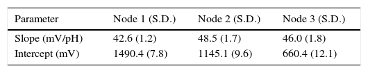
The WCSN was evaluated considering three aspects: sensor precision and accuracy and wireless network performance. Results in this section use standard pH 4 and 7 solutions as an example. Calibration results employing other combinations of pH values were similar. Table 1 shows response characteristics for the three nodes. The repeatability of calibration data (slope and intercept) was high as indicated by the values of the standard deviation. Table 1 summarizes results for 10 repetitions.
These values were programmed by default in each node. During calibration, the slope must be between 43 and 55mV/pH. If the computed value falls outside this range, the LCD shows an error message and the node uses default calibration values. Otherwise, the node stores the most recent slope value.
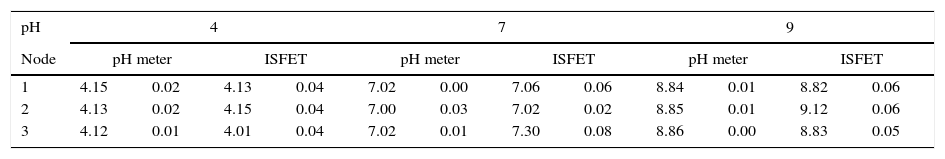
3.1Repeatability and accuracy of pH measurementsTests measured three pH solutions (4, 7 and 9) for each node, in order to establish the precision and accuracy of ISFET sensors and the measurement system. Results were compared with those from a pH commercial meter WTW Multi3420. Test employed ten repetitions for each pH value. Measurements were done at room temperature using the same solutions and conditions for both the pH meter and the nodes. Table 2 summarizes results of this test. As shown, the repeatability of pH data represented by the standard deviation agrees with the commercial pH meter.
pH value and standard deviation for each node for three different buffer solutions.
| pH | 4 | 7 | 9 | |||||||||
|---|---|---|---|---|---|---|---|---|---|---|---|---|
| Node | pH meter | ISFET | pH meter | ISFET | pH meter | ISFET | ||||||
| 1 | 4.15 | 0.02 | 4.13 | 0.04 | 7.02 | 0.00 | 7.06 | 0.06 | 8.84 | 0.01 | 8.82 | 0.06 |
| 2 | 4.13 | 0.02 | 4.15 | 0.04 | 7.00 | 0.03 | 7.02 | 0.02 | 8.85 | 0.01 | 9.12 | 0.06 |
| 3 | 4.12 | 0.01 | 4.01 | 0.04 | 7.02 | 0.01 | 7.30 | 0.08 | 8.86 | 0.00 | 8.83 | 0.05 |
Note all ISFET values in Table 2 were extrapolated employing linear fit parameters obtained during the calibration process. Additionally, the accuracy was calculated as the relative difference between the pH value obtained with the ISFET node and with the pH meter. Therefore, accuracy is below 5%, which is acceptable for different instruments of measurement.
3.2Wireless network testsThe second test measured the number of packets lost when the number of transmitting nodes increased from 1 to 3. Each node transmitted 100 packets and experiments were repeated five times. When using the protocol explained in Fig. 7, where each node sends a new packet every 10s, there were no packet losses. The measurement of pH in surface waters may tolerate higher sampling periods. Therefore, if increasing the sampling period, new nodes can join the network without creating collisions. The three nodes were tested using 1mW transmission power, as in study (Berdugo et al., 2012).
One additional test was performed in order to verify the maximum radio range. One node was measuring pH values inside a laboratory. Transmission power employed was 1W. The receiver node was placed in different positions outside the laboratory. Fig. 9 shows different locations employed during tests. The square is the transmitter. Circles show the smallest reception levels. The triangle shows location with the best reception level and the diamond shows medium level.

Fig. 9 shows maximum distance was 474m between transmitter and receiver, but the signal level was small. Best reception occurred inside the laboratory building, at 30m through metal doors and concrete walls. Every Xtend modem in the WCSN employs one omnidirectional antenna; hence, they are transmitting information in all directions. Note reception was possible when testing in parking lots and different roads. Nonetheless, because of the obstacles, the system was working in the gray area of communication systems, where packet losses are between 10% and 90% (Aguirre et al., 2014). Additionally, tests verified locations inside different buildings, going south from the transmitter. However, there was no packet reception in these locations. The results are expected since signal had to propagate through concrete, glass, metal and trees, thus significantly reducing radio range.
Additionally, the test provided insights on stability performance of the node. Fig. 10 shows measurements for one node taken from 10 AM to 14:10 PM. Figure shows typical ISFET behavior, with a drift during the first two hours and a stabilized drift after that time. Note there is a gap in data from 10:50 AM to 12:54 PM. During this time, receiver position did not allow data reception.
4Conclusions
This paper demonstrates the performance of a chemical sensor network for pH monitoring. The pH values and the repeatability are comparable with a commercial sensor. This result corroborates the feasibility of ISFET technology as pH sensors and the viability of the measurement circuit. The major part of systems employed in the literature report transmission distances smaller than 30m. The Xtend radio modems used in this work allow transmission up to 474m through obstacles such as buildings and trees. Therefore, the application could be implemented in longer distances, with unobstructed line of sight.
Using a TDMA algorithm and sending information every 10s, the network presented no packet losses. Since pH monitoring in water can be performed through larger periods, the system can increase the number of nodes without increasing packet losses.
Human interface was designed and implemented in order to fulfill calibration required by chemical sensors. This functionality also allows each node to work as stand-alone pH meter, independent of the wireless network.
Conflict of interestThe authors have no conflicts of interest to declare.
This research was funded in part by Direction of Research, Development and Innovation (DIDI) at Universidad del Norte through project 2011-1154, by CYTED Project number P509AC0376 and by Colciencias-CSIC Exchange Grant 2011. We would like to thank Antonio Ramos and Ángela Sierra for their help in using Chemistry and Water Labs at Universidad del Norte.
Peer Review under the responsibility of Universidad Nacional Autónoma de México.