


In order to effectively analyze and forecast the global CO2 concentration, a collaborative fuzzy-neural agent network is constructed in this study. In the collaborative fuzzy-neural agent network, a group of autonomous agents is used. These agents are programmed to analyze and forecast the global CO2 concentration using the fuzzy back propagation network (FBPN) approach based on their local views. A collaboration mechanism is established to communicate the settings and forecasts of these agents, and to derive a single representative value from these forecasts using a radial basis function network. The real data were used to evaluate the effectiveness of the collaborative fuzzy-neural agent network approach.
It is concerned that the accumulation of greenhouse gases, especially CO2, in the atmosphere leads to undesirable changes of the global climate. The global CO2 concentration, derived from measurements of CO2 concentration in air bubbles in the layered ice cores drilled in Antarctica and from atmospheric measurements, is considered to be one of the most important causes of global warming, and should be closely monitored, accurately forecasted, and controlled (National Assessment Synthesis Team, 2000). For example, according to the measurement by Earth System Research Laboratory Global Monitoring Division, the monthly average Mauna Loa CO2 concentration of October 2014 was 395.93ppm, while that of October 2013 was 393.66ppm (Earth System Research Laboratory Global Monitoring Division, 2014). Long-term environmental planning is usually based on such figures. For example, targets are set for reducing CO2 emissions around the world. In addition, the range of the global CO2 concentration is also important, for which the narrowest range should be determined so that the global CO2 concentration is neither over-estimated nor under-estimated (Chen & Wang, 2011). Otherwise, there is a risk of energy shortage, or the government may raise budget unreasonably.
Agent network is remarkable for its promising use for human-unattended tasks (Wang et al., 2008). Wang et al. (2008) mentioned that there are two performance measures in evaluating the optimal performance of an agent network – the network lifetime finally acquired and the total information finally collected. However, in different circumstances, targets may not be the same. In Yan, Zheng, & Lin (2009), it was found that opportunistic collaboration can reach better performance than direct transmission.
Agent network-based data analyses have become an important field of research, and new applications are expected to appear. For example, a synchronized agent network system was developed in Uchimura et al. (2007) for vibration measurement. It is now possible to obtain environmental information from difficult-to-reach places (Endo et al., 2008). In Morreale's opinions, agent networks have potential applications to urban telehealth (Morreale, 2007). Recently, Fukushima nuclear power plant incident led to the rise in the radiation level in the plant. This environment is extremely dangerous for human operators to enter, and some robots have been sent to monitor the radiation level. These examples tell us the importance of autonomous agents for detecting atmospheric conditions.
On the other hand, fuzzy agents have been used in various fields. For example, in Lee and Pan (2004), three types of agents, including meeting negotiation agent, fuzzy inference agent, and genetic learning agent, are designed to help search and decide the suitable meeting time. In Zarandi, Pourakbar, & Turksen (2008), an agent-based system is developed to minimize the total costs and to reduce the bullwhip effect in a supply chain. Each agent used a hybrid of the modified Hong fuzzy time series, genetic algorithm (GA), and a back propagation neural network (BPN) to forecast the trend in the collected data. In Lu and Sy (2009), some fuzzy inference rules were established for fuzzy agents to make process control decisions, so as to quicken the response to customers’ requests.
The global CO2 concentration forecasting is a long-standing research task and we believe that there is still room for further development. For this reason, in order to effectively analyze and forecast the global CO2 concentration, a collaborative fuzzy-neural agent network is constructed in this study. In the collaborative agent network, a group of agents is used. These agents are programmed to forecast the global CO2 concentration based on their local views, and may not share the raw data they own with each other. A collaboration mechanism is therefore required to aggregate their forecasts. Each agent is equipped with a fuzzy back propagation network (FBPN) reasoning module to forecast the global CO2 concentration, based on the agent's setting. Each agent communicates its setting and forecasting results to other agents through the central control unit. After receiving this information, if it reveals that the forecasting performance of an agent is very prominent, the others may change their settings, so that their settings and forecasting results will move closer. Similar iterative approaches have been used in Bhattacharya and Vasant (2007), Peidro and Vasant (2011), etc. To facilitate the collaboration process and derive a single representative value from the forecasts by the agents, the central control unit is equipped with a radial basis function network (RBF) reasoning module. Finally, the whole system is built on a centralized point-to-point (P2P) communication architecture. The real data of the global CO2 concentration are used to evaluate the effectiveness of the collaborative fuzzy-neural agent network.
2. MethodologyThe operational procedure of the collaborative fuzzy-neural agent network consists of several steps that will be described in the following sections:
- 1.
The collaborative fuzzy-neural agent network starts from the formation of a group of agents.
- 2.
The administrators of these agents specify their requirements for certain aspects of forecasting that are incorporated into the agents’ FBPN settings.
- 3.
Each agent analyzes and forecasts the global CO2 concentration based on its own view.
- 4.
Each agent communicates its setting and forecasting results to other agents through the central control unit. After receiving these, an agent may be affected to modify its setting.
- 5.
To arrive at a representative value from the forecasting results, a RBF network is employed.
- 6.
The collaboration process is terminated if the improvement in the aggregate forecasting performance becomes negligible. Otherwise, return to step 3.
The system diagram of the proposed methodology is shown in Figure 1. The variables and parameters that will be used in the proposed methodology are defined in Table 1. All fuzzy variables and parameters are expressed with triangular fuzzy numbers (TFNs), e.g. C˜t=Ct1,Ct2,Ct3. In fact, only the lower and upper bounds, not the membership function, of C˜t are of concern. For this reason, it does not matter whether the membership function is linear or nonlinear.

The Nomenclature Table.
| Variable/Parameter | Meaning |
|---|---|
| at | The actual value (after normalization) of the global CO2 concentration at period t |
| C˜t | The global CO2 concentration forecast at period t |
| o˜(t) | The FBPN output, which is the normalized forecast of the global CO2 concentration at period t, i.e. o˜(t)=NC˜t |
| h˜l(t) | The output from hidden-layer node l, l = 1 ∼ L |
| w˜lo(t) | The weight of the connection between hidden-layer node l and the output node |
| w˜klh(t) | The weight of the connection between input node k and hidden-layer node l; k = 1 ∼ K; l = 1 ∼ L |
| θ˜lh(t) | The threshold for screening out weak signals by hidden-layer node l |
| θ˜°(t) | The threshold for screening out weak signals by the output node |
In the collaborative fuzzy-neural agent network, each agent uses the FBPN reasoning module to forecast the global CO2 concentration, based on its local view. The theoretical background of the FBPN approach is explained as follows.
Although there have been some more advanced artificial neural networks, such as compositional pattern-producing network, cascading neural network, and dynamic neural network, a well-trained FBPN with an optimized structure can still fit any complex relationship very precisely (Eraslan, 2009; Firoze, Arifin, & Rahman, 2013; Babaei, Suratgar, & Salemi, 2013; López et al., 2013). That is why it is selected in this study:
- 1.
K inputs, corresponding to the levels of the global CO2 concentration K periods ago. To facilitate the search for solutions, it is strongly recommended to normalize the inputs into a range narrower than [0 1] (Chen, 2008).
- 2.
The FBPN has only one hidden layer. Additional hidden layers may simply enable the memorization of the training data, not a true reflection of the actual input-output relationship. The number of nodes in the hidden layer is chosen from 1 to 2K after trying each of them.
- 3.
The output from the FBPN is the normalized forecast of the global CO2 concentration.
- 4.
The activation function used for the hidden layer is the hyperbolic tangent sigmoid function, while for the others is the linear activation function.
- 5.
10,000 epochs will be run each time. The start conditions will be randomized to reduce the possibility of being stuck on local optima. In this way, it is possible to achieve a globally optimal solution. Nevertheless, even if the original forecasts are just locally optimal, after collaboration these forecasts can still be improved considerably, showing that the proposed methodology is robust to the so-called “bad experts”.
- 6.
Early stopping: After each 100 training epochs, the FBPN is applied to the testing data. The training process will also stop if the testing performance begins to deteriorate.
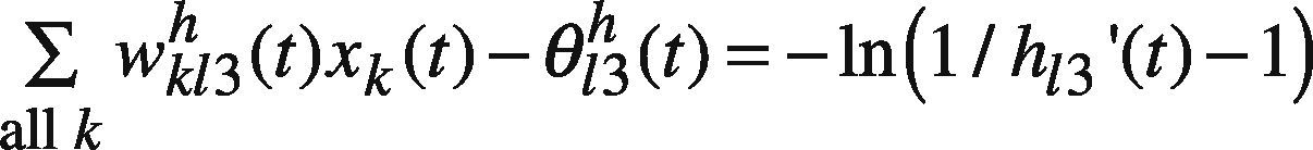
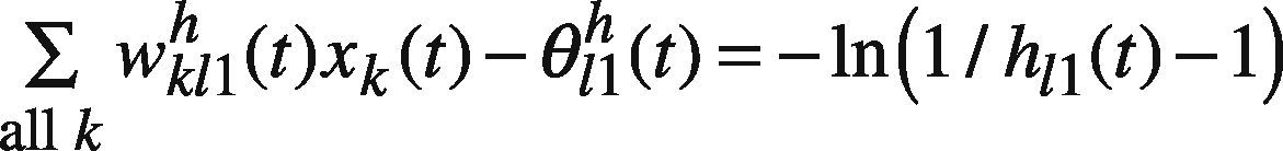
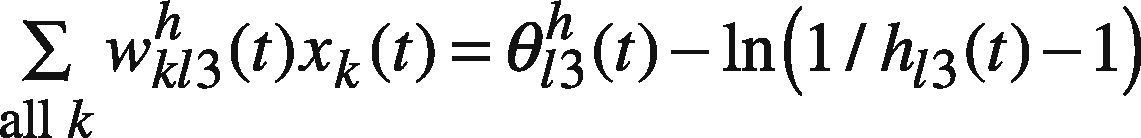
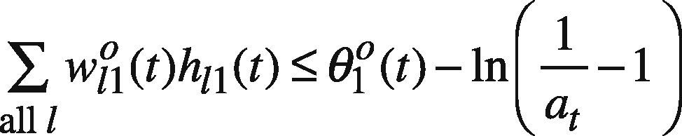
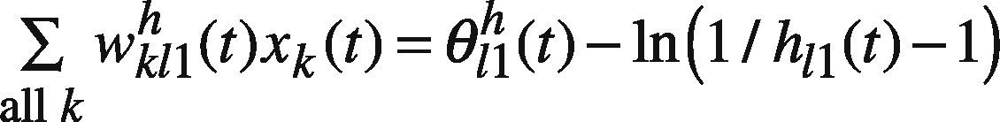
The training of the FBPN reasoning module is decomposed into three subtasks: determining the center, upper, and lower bounds of the parameters. First, to determine the center of each parameter (such as wkl2h(t), θl2h(t), wl2o(t), and θ2o(t)), numerous algorithms can be used, such as the gradient descent algorithm, the conjugate gradient algorithm, the scaled conjugate gradient algorithm, the Levenberg-Marquardt (LM) algorithm, the Broyden-Fletcher-Goldfarb-Shanno algorithm, the gradient descent with momentum and adaptive learning rate back propagation algorithm, the resilient back propagation algorithm, and the TD-Gammon algorithm. Eraslan (2009) provided a comparison of these algorithms. In this study, the LM algorithm is applied due to its efficiency.
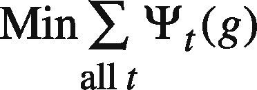
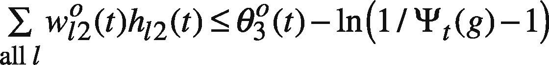
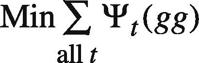
Subsequently, the following goal programming (GP) problem is solved to determine the upper bound of each parameter (e.g. wkl3h(t), θl3h(t), wl3o(t), and θ3o(t)) (Chen & Wang, 2012; Chen, 2012):
(GP I)
subject to


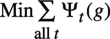
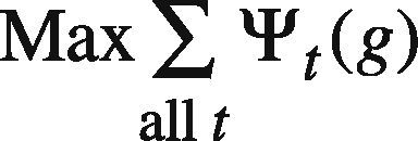
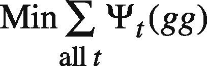
At first, ψt(g) is set to ct2(g)+Δt(g) where Δt(g) is a randomly generated nonnegative value. If any feasible solution can be found, Δt(g) is re-generated so that ∑all tψt(g) can be reduced. In this way, the goal programming problem is solved a few times. In these optimization results, the best one giving the minimal ∑all tψt(g) is chosen.
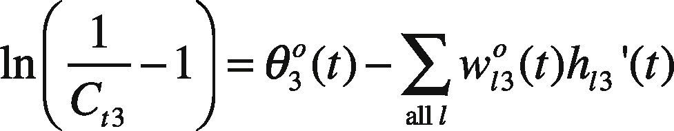
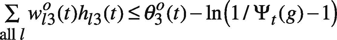
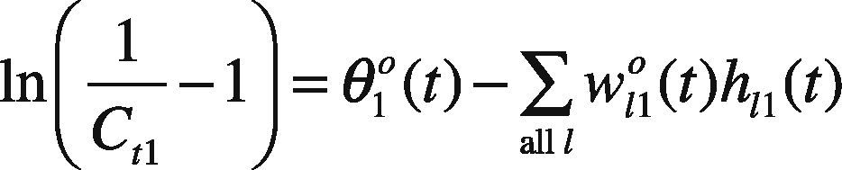
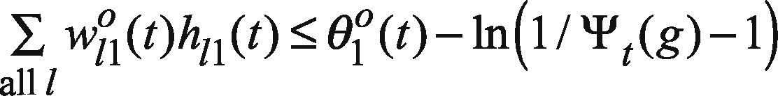
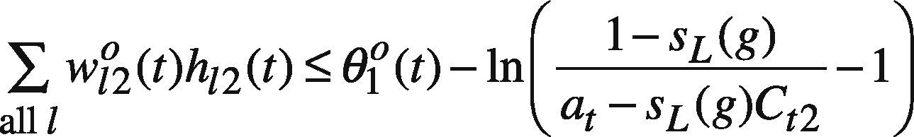
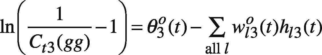
Model GP I is a nonlinear problem that is not easy to solve. To simplify the problem solving, assume only the threshold on the output node, i.e. θo(t), is fuzzified as (θ1o(t), θ20(t), θ3o(t)), while the other network parameters are equal to their centers. As a result, model GP I is simplified as
(Simplified GP I)
subject to
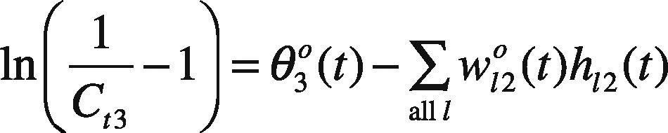
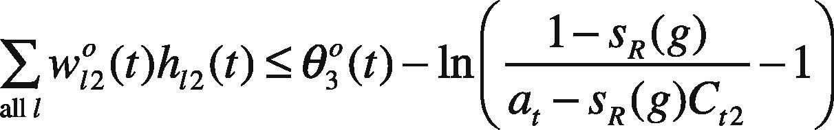


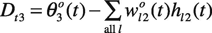
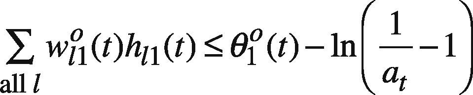
where ∑all lw120(t)h12(t), ln1−SR(g)at−SR(g)C12−1, and ln1at−1 are all constants. In addition, ln1Ct3−1 can be replaced by a new variable Dt3,
In this way, the problem becomes a linear one.
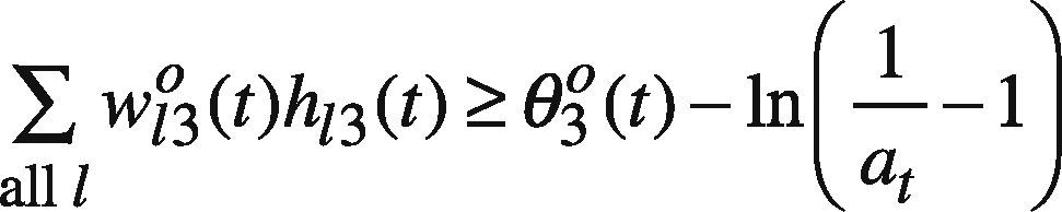
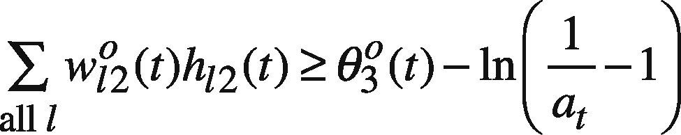
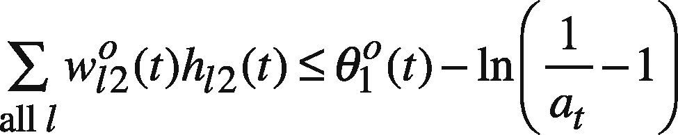
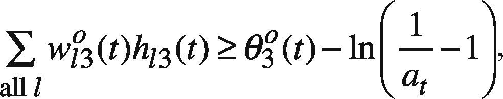
In a similar way, the following GP problem is solved to determine the lower bound of each parameter (e.g. wkl1h(t), θl1h(t), wl1o(t), and θ10(t)):
(GP II)
subject to


At first, ψt(g) is set to ct2−Δt(g) where Δt(g) is nonnegative and randomly generated. If any feasible solution can be found, Δt(g) is re-generated so that ∑all tΨt(g) can be increased. In this way, the GP problem is solved some times. In these optimization results, the best one giving the maximal ∑all tΨt(g) is chosen.
Model II can be simplified as:
(Simplified GP II)
subject to


All actual values will fall within the ranges of the fuzzy forecasts. However, such a “robust” property no longer holds under a distributed environment in which an agent has only partial access to the data. To solve this problem, the forecasting results by all agents can be communicated to each other, so that they can modify their settings, and generate more robust forecasts as if all data are taken into account. To this end, the GP problems are modified so that a collaborative formulation can be proposed in the next section.
2.2. Collaboration Among AgentsThe setting of an agent is indicated with VSg = { ψt(g), SR(g), SL(g)}, g ∈ [1 G], and will be packaged into information granules, which are then encoded using extensible markup language (XML). Subsequently, a software agent is used to transmit information granules among agents through a centralized P2P architecture. The communication protocol is as follows:
Input Agent g, 1 ≤ g ≤ G, provides input data C˜t for T periods, where n ≤ t ≤ T + n – 1. In case of computing the FBPN output, the setting vector VSg is public.
Output Agent g, 1 ≤ g ≤ G, learns DC˜t−atat without anything else, where DC˜t is computed using the center-of-gravity method (Wrather & Yu, 1982).
After receiving this information, if it reveals that the forecasting performance of an agent is very prominent, the others may change their settings, so that their settings will move closer. In addition, if an agent does not have an access to the data of a specific period or the data are not reliable, it should respect the forecasts by other agents that have accesses to the data.
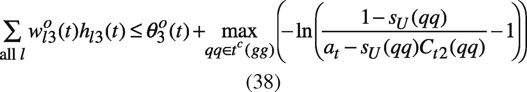
After communication agent g refits the corresponding FBPN with the following GP models, based on Chen and Wang's fuzzy collaborative forecasting method (Chen & Wang, 2014):
(GP III)
subject to


(GP IV)
subject to


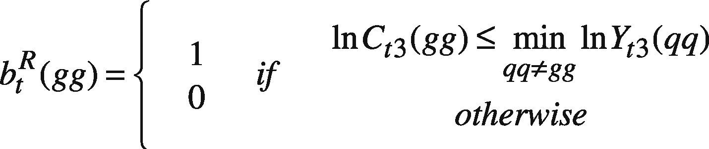

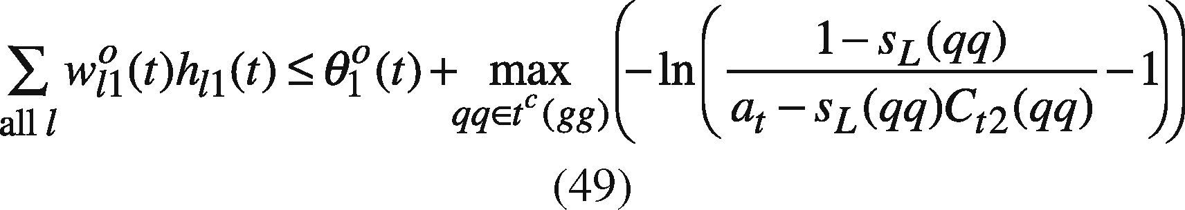

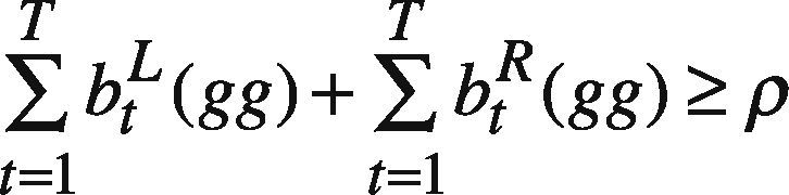
where VSqq=ψt(qq), SR(qq), SL(qq) is the setting of agent q and so on, following the notations suggested by Pedrycz (2008); t(qq) includes the time indexes of all data in the part assessed by agent q; tc(qq) is the complement of t(qq), i.e. tc(qq) = [1 T]-t(qq); s(ii) is the satisfaction level requested by agent i. btL(gg), and btR(gg) are equal to 1 if the forecast by agent g is better than those by others, on the left-hand and right-hand sides, respectively. Constraint (37) and (38) force the upper bound on the fuzzy forecast to be greater than those made by other agents for a period the datum is lacking. On the contrary, in (48) and (49), the lower bound should be less than those made by other agents for the same period.
If there are L agents, then after incorporating the users’ views into the FBPN reasoning modules, there will be at most 2L GP problems to be solved. After solving every two GP problems, the optimal solution is used to configure the corresponding FBPN reasoning module. Eventually, there will be at most L FBPNs, each of which generates a forecast of the global CO2 concentration.
2.3. Aggregating the Fuzzy Forecasts With a RBFSubsequently, a RBF is used to aggregate and defuzzify the fuzzy forecasts from a few agents to arrive at a representative value. The RBF network has three layers: the input, hidden (middle), and output layers. Inputs to the RBF are the three corners of the fuzzy forecasts. For example, if a fuzzy forecast is (a,b,c), then the inputs to the RBF are a, 0, b, 1, c, and 0. As there are G agents, the number of inputs to the RBF is 6G. The reason is simple – aggregation results in a convex domain, and each point in it can be expressed with the combination of corners. Most of the defuzzification algorithms do the same thing.
As mentioned earlier, all the input parameters are normalized into a range narrower than [0 1]. Each input is assigned to a node in the input layer and passed directly to the hidden layer without being weighted. The transfer function used for the hidden layer is Gaussian transfer function:
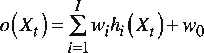
where Xt = [xt1,…, xtr] is the input vector; hi(Xt) is the output from the i-th node in the hidden layer, i = 1 ∼ I; x˜tj and σi are the center and width of the i-th RBF unit for input variable j, respectively. The output layer uses the linear transfer function:
For determining the parameter values, k-means (KM) is first used to find out the centers of the RBF units. Subsequently, the nearest-neighbour method is used to determine their widths (Ahmadaali, Liaghat, Haddad, & Heydari, 2013). The weights of the connections can be obtained by linear regression.
3. Application and AnalysesTo demonstrate the application of the proposed methodology, the real data of the global CO2 concentration were used. From 2004 to 2013, the average annual increase in the global CO2 concentration was 2.1ppm per year (CO2Now.org, 2013). Three agents, each was programmed on a PC with Intel Core i5-3470 CPU and 8GB RAM, forecasted the global CO2 concentration from 2005∼2009 based on their local views. To configure the FBPN reasoning modules, there were six GP problems to be solved. From the optimization result of every two GP problems, a corresponding FBPN reasoning module was configured. All three FBPN reasoning modules were applied to forecast the global CO2 concentration. Each agent communicated its setting and forecasting results to other agents with the aid of the central control unit. The central control unit selectively transmitted information between agents, to maximize the efficiency of collaboration. After receiving this information, each agent adjusted its setting according to the two collaboration mechanisms. Finally, a RBF network was applied to derive the representative value, i.e. the crisp global CO2 concentration forecast, from these fuzzy forecasts.
In the equipped FBPN reasoning module, the setting of an agent was stored into a database which was constructed using Microsoft Excel 2003. The Optimization Toolbox of MATLAB (2006a) was applied to solve the GP problems. To exchange and synchronize the data between the database and the optimizer, the Excel Link add-in of MATLAB was used, which communicates between the Excel workspace and the MATLAB workspace and positions Excel as a front end to MATLAB. Finally, the Neural Network Toolbox of MATLAB (2006a) was applied to implement the FBPN approach. We considered the following performance measures: root mean squared error (RMSE), mean absolute error (MAE), mean absolute percentage error (MAPE), and the hit rate (i.e. the percentage that the actual value is contained in the fuzzy forecast).
The actual values of the global CO2 concentration are shown in Figure 2. If an agent has the integral access to the data, then the forecasting results by the FBPN reasoning module will be like Figure 3. Obviously, the FBPN reasoning module can provide a perfect fit for the data collected. A fuzzy global CO2 concentration forecast is defuzzified with the COG formula:


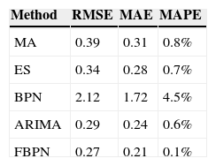
To make a comparison with some existing approaches, MA, ES, BPN, and ARIMA were also applied to forecast the global CO2 concentration. The forecasting accuracy achieved by applying these approaches were recorded and compared in Table 2. The accuracy of forecasting the global CO2 concentration, measured in terms of RMSE, of the FBPN reasoning module, was significantly better than those of the traditional approaches by achieving a 31% reduction in RMSE over the comparison basis – MA. The advantages over ES, BPN, and ARIMA were 21%, 87%, and 7%, respectively. The accuracy of the FBPN reasoning module with respect to MAE or MAPE was also significantly better than those of the other approaches.
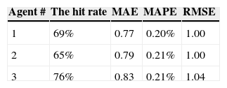
However, these agents only had partial access to the data. Therefore, the forecasting results by the three agents before collaboration are shown in Figure 4. Their forecasting performances are compared in Table 3.

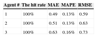
In the first communication, the exchange of information among the three agents is not limited. After receiving the forecasting results of other agents, some of them changed their settings. The central control unit compared the Euclidean distances between the settings of two agents before and after communication. Two agents favor each other if the distance between their settings is reduced after collaboration. On the contrary, if the distance between the settings of two agents increases after collaboration, then they disfavor each other. Subsequently, in the next communication, the exchange of information between two agents will only be done if they lack consensus and favor each other. On the contrary, two agents will be allowed to exchange forecasts if they disfavor each other and their consensus is high. After collaboration, the forecasting performances of the three agents were considerably improved (see Table 4).
Subsequently, a RBF was used by the central control unit to aggregate and defuzzify the fuzzy forecasts from the three agents to arrive at a representative value. The aggregate forecasting performance was as follows:
- •
The hit rate: 100%
- •
RMSE: 0.34
- •
MAE: 0.25
- •
MAPE: 0.07%
The aggregate forecasting performance was clearly superior to those of the three agents (see Fig. 5), and was quite close to that when the agents have the integral access to the data, which confirmed the effectiveness of the RBF network. It was not easy since the three agents did not share the raw data they owned with each other.

To further elaborate the effectiveness of the proposed methodology, it was also compared with the seasonal recurrent support vector regression model with chaotic artificial bee colony (SRSVRCABC) algorithm (Hong, 2011) that is composed of four major steps: dividing training data into different sizes of fed-in and fed-out subsets, determining the values of parameters using the chaotic artificial bee colony (CABC) approach, adjusting the parameters using the back propagation algorithm, and seasonal adjustment. The proposed methodology is an external collaboration method that seeks the consent of all agents. In contrast, the SRSVRCABC algorithm is an internal collaboration method that groups artificial bees to effectively search the solution space. The comparison results are shown in Figure 6. The proposed methodology still outperformed the SRSVRCABC algorithm.
4. Conclusions and Directions for Future Research
A positive relationship between global warming and the global CO2 concentration has been confirmed in a lot of studies. However, the magnitude of this effect is highly uncertain and difficult to be forecasted using the available methods. In order to effectively forecast the global CO2 concentration, a collaborative fuzzy-neural agent network is constructed in this study. In the collaborative fuzzy-neural agent network, each agent uses the FBPN reasoning module to forecast the global CO2 concentration, based on its local view. The FBPN reasoning module is simplified from the model proposed by Chen (2012). In addition, its effectiveness is enhanced using Chen and Wang's fuzzy collaborative forecasting method (Chen & Wang, 2014). Each agent communicates its setting and forecasting results to other agents with the aid of the central control unit. After receiving this information, the agents may change their settings, based on two collaboration mechanisms. In addition, if an agent does not have the access to the data of a specific period or the data are not considered reliable, the agent should respect the forecasts by other agents that have access to the data.
According to the experimental results, it is found that:
- 1.
The hit rate, MAE, MAPE, and RMSE of forecasting the global CO2 concentration by each agent was not satisfactory. The poor setting of an agent may be the first reason. Another reason is that the QP problems are not easy to solve; sometimes only local optimal solutions can be found. The simplified QP models provide a solution to this problem. However, other FBPN methods that are more effective are still needed. In addition, a more effective communication mechanism that can provide agents more information on how to improve their forecasting performances is also helpful.
- 2.
The aggregate forecasting performance was considerably improved through the agents’ collaboration without sharing the raw data they owned.
- 3.
It is therefore possible to forecast the global CO2 concentration precisely and accurately using a group of local agents governed by a centralized P2P network.
In future studies, more sophisticated fuzzy-neural agent networks or collaboration mechanisms can be developed.
FundingThis study was financially supported by the Ministry of Science and Technology, Taiwan.