


This paper presents a simple and systematic approach to formulate the inverse position problem of a Schönflies parallel manipulator. As a result, the inverse position problem is solved in closed form and leads directly to the automatic generation of the workspace of the manipulator. Additionally, a systematic velocity analysis is also presented, which allows to detect and characterize all the singularities related to this manipulator.
Although several studies of workspace have been performed for many types of manipulators (Abdel-Malek, Adkins, Yeh, & Haug, 1997; Bohigas, Manubens, & Ros, 2012; Bonev & Ryu, 2001; Davidson & Hunt, 1987; Gosselin, 1990; Gupta & Roth, 1982; Lee & Lee, 2012; Macho, Altuzarra, Pinto, & Hernández, 2013; Merlet, 1999; Pernkopf & Husty, 2006), the search of a general and precise definition of the workspace of a robot is a subjective task. Perhaps it is because the workspace of a manipulator may be described with respect to its ability to reach points, lines, planes or three-dimensional bodies attached to the mobile platform. Hence the simplest definition of workspace is that related to positioning manipulators. For this simple case, the workspace is defined as the volume of space that a point of the end effector can reach. However, when the physical entity attached to the mobile platform is a line, a plane or a 3D object, the problem related to the graphical visualization of the corresponding workspace is not an easy task. Therefore, due to the particular features of a Schönflies motion, namely, a spatial translation and a rotation about a fixed axis, this paper deals with the so-called reachable workspace, i.e., the volume of space within every point can be reached by the mobile platform in at least one orientation.
Furthermore, qualitative and quantitative studies of workspaces are important because they may be used to: (a) yield useful insights about the kinematic architecture of the manipulator in the design stage, (b) lead to criteria for the evaluation of different types of manipulators, (c) assist in the planning of desired tasks in favorable zones, and (d) avoid dangerous collisions with objects. Moreover, even for the simplest robotic system, the robot controller program must control the motions of the manipulator and mobile platform to carry out a task in the specific workspace.
On the other hand, a first-order singularity analysis deals with those problems encountered during the solution stage of the velocity analysis of a manipulator (Hao & McCarthy, 1998; Gosselin & Angeles, 1990; Altuzarra, Pinto, Avilés, & Hernández, 2004; Amine, Masouleh, Caro, Wenger, & Gosselin, 2012; Ghosal & Ravani, 2001; Zlatanov, Fenton, & Benhabib, 1995). As a result of such problems, degrees of freedom may be instantaneously gained or lost. Particularly dangerous are those manipulator's configurations where degrees of freedom are gained in an unexpected way. There, the manipulator may danger its own environment, including adjacent equipment and human beings. Moreover, certain types of singularities divide the whole workspace into several regions. Hence it is important to detect all the singularities and to know about their distribution in the workspace of the manipulator.
In particular, in Amine, Masouleh, Caro, Wenger, and Gosselin (2012) it is reported a singularity analysis of 3T1R parallel manipulators with identical limb structures, where a specific case study is fully detailed. However, the kinematic structure of the manipulator described in that case study is not equal to the kinematic architecture of the manipulator reported in the present paper. Moreover, the singularity analysis reported in (Amine et al., 2012) is based on Grassmann-Cayley Algebra, whereas the singularity analysis introduced in the present paper is based only on classical concepts of vectors and Linear Algebra, which results in a simpler approach. Furthermore, due to the exhaustive nature of the approach proposed in the present paper, a set of 95 singularity configurations are mathematically identified and geometrically characterized. Finally, the singularities are plotted into the manipulator's workspace, thus enlightening their geometric meaning.
From the foregoing discussion, the contribution of this paper will be focused on four directions: (a) a closed form solution of the inverse position problem, (b) a workspace generation scheme, (c) a systematic velocity analysis, and (d) characterization and detection of all the singularities and their distribution in the reachable workspace of a Schönflies parallel manipulator. It is expected that these contributions may be useful for an adequate planning of tasks.
2The Schönflies parallel manipulatorFigure 1 shows a spatial 4-dof parallel manipulator whose mobile platform generates a Schönflies motion.

Referring to Figure 1, it may be noted that the moving platform (link 5) is connected to a fixed base (link 0) by four nonidentical legs. The objective is to have a Schönflies parallel manipulator with different actuation schemes, i.e., using two rotatory actuators and two prismatic actuators. As a result, the Jacobian matrices will not be homogeneous in terms of units, see Eq. (41). It is expected to conduct an analysis of this particular type of Jacobian matrices and their relation with dexterity indices. This will be the research topic in a forthcoming paper.
2.1Kinematic architecture of the legsThe kinematic architecture1 of the legs involves two types of legs:
- (a)
The first type of leg is made up of five revolute joints, see the first (O1-A1-B1-C1-D1-1) and the third (O3-A3-B3-C3-D3-3) legs shown in Figure 1. In this leg, the second and fifth joint axes are parallel to the first joint axis, whereas the fourth joint axis is parallel the third joint axis. Moreover, the third joint axis intersects the second perpendicularly, and the fifth joint axis intersects the fourth perpendicularly. Furthermore, there is an offset distance between the first and the second joint axes. A rotational actuator is used to drive the first joint of the leg where the motor is installed on the fixed platform.
- (b)
The second type of leg is made up of one prismatic joint and four revolute joints, see the second (O2-A2-B2-C2-D2-2) and the fourth (O4-A4-B4-C4-D4-4) legs shown in Figure 1. In this leg, the second and fifth joint axes are parallel to the first joint axis, whereas the fourth joint axis is parallel the third joint axis. Moreover, the third joint axis intersects the second perpendicularly, and the fifth joint axis intersects the fourth perpendicularly. Furthermore, there is an offset distance between the first and the second joint axes. The first moving link of this leg is driven by a translational actuator mounted on the fixed platform.
For the spatial parallel manipulator shown in Figure 1, the four fixed points O1, O2, O3, and O4 define the geometry of the fixed platform, and the four moving points 1, 2, 3, and 4 define the geometry of the mobile platform. Although the particular manipulator's platforms shown in Figure 1 are symmetrical, it should be noted that both, the fixed platform and the mobile platform, may be arbitrary planar quadrilaterals, see Figure 2.

Additionally, Figures 3–6 show the link lengths and joint variables related to the four legs. It is important to mention that unit vectors e1, e2, e3 and e4 denote the joint axes of those revolute joints that join links 12 and 13, 22 and 23, 32 and 33, and 42 and 43, respectively.


In summary, the pose of the mobile platform can be specified in terms of the position of point P, and an orientation angle, namely, ϕ, see Figure 2. Moreover, the origin of the fixed coordinate frame X0Y0Z0 is located at point O.
3Kinematic position analysisThe objective of this section is to formulate the inverse position problem associated with the manipulator under study. On the one hand, it should be noted that angles φ1, φ2, φ3, φ4, β1, β2, β3, β4, γ1, γ2, γ3 and γ4 are passive joint variables, whereas θ1, p2, θ3 and p4 are active joint variables, see Figures 3–6. On the other hand, rP/O=(x, y, z)T is the position vector of moving point P with respect to fixed point O, which is measured in the X0Y0Z0 coordinate frame, and ϕ denotes the rotation of the mobile platform about the Z0 axis, see Figure 2.
3.1Constraint equationsIn order to obtain the so-called constraint equations, the procedure begins by writing a loop-closure equation for each leg:
where rj/k stands for the position vector of point j with respect to point k.
Writing equation (1) for i=1, 2, 3, 4, and taking the X0Y0Z0 coordinate frame as a reference, it is obtained that:
which are the constraint equations sought.3.2Handling of the constraint equations


The approach can be started by focusing on the fact that equations (2)–(13) are linear in the sines and cosines of passive joint variables φ1, φ2, φ3, and φ4. Thus, from simultaneous solution of equations (2), and (3), (5), and (6), (8), and (9), (11), and (12), respectively, it is found that:


Introducing the trigonometric identities sin2φi+cos2φi=1, fori=1, 2, 3, and 4, Eqs. (14)–(21) become:


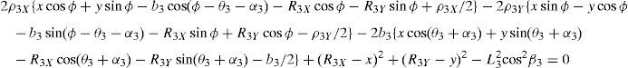

Additionally, Eqs. (4), (7), (10), and (13) are solved for sinβi, and then squared. Next, Eqs. (22)–(25) are solved for cos2βi. Then, by introducing the trigonometric identities sin2βi+cos2βi=1, for i=1, 2, 3, and 4, the following equations are obtained:
where


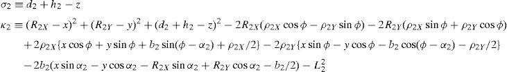
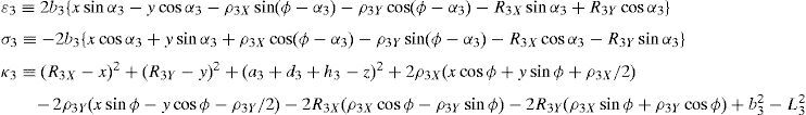
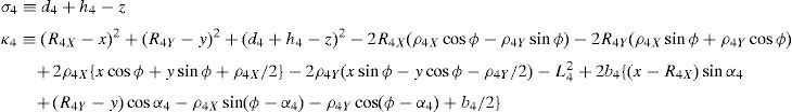
At this point, it should be mentioned that equations (26)–(29) can be solved for the input displacements, namely, θ1, p2, θ3 and p4, respectively, which is a procedure usually known as inverse position problem.
4Workspace generationThe workspace of the manipulator will be defined here as the volume of space that point P of the mobile platform can reach in at least one orientation. Thus, the manipulator's workspace will be composed by a large set of points Pi, whose Cartesian coordinates are given by xi, yi, zi. At each point Pi, the mobile platform will have a common orientation angle, namely, ϕG.
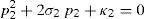
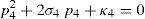
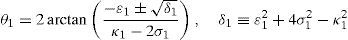
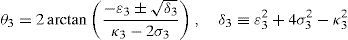
In order to detect which point Pi is contained within the manipulator's workspace, the following approach is proposed. Firstly, if the workspace is given in terms of the Cartesian coordinates x, y, z and the orientation angle ϕ, then equations (26)–(29) can be solved for the input displacements, namely, θ1, p2, θ3 and p4, respectively. Analyzing equations (26)–(29), it can be observed that equations (27) and (29) are quadratic in p2 and p4, respectively. Moreover, equations (26) and (28) are trigonometric expressions that can be converted into quadratic equations in τ1≡tan(θ1/2) and τ3≡tan(θ3/2), respectively. Thus, the solution process can be summarized as follows:


Then, a point Pi (accompanied with a given orientation angle ϕ=ϕG) will be part of the workspace if and only if the following constraints:
are simultaneously satisfied. Such conditions guarantee that at least one set of real input displacements exist for that point.
In summary, the workspace is generated by considering a three dimensional grid of points Pi equipped with conditions (34). As a result, the plots shown in Figures 7 and 8 were obtained.


Figures 7 and 8 were generated by considering the following numerical values of the design parameters: R1X=180, R2X=180, R2Y=0, R3X=0, R3Y=−180, R4X=−180, R4Y=0, ρ1X=181.10, ρ2X=13.25, ρ2Y=119.26, ρ3X=176.69, ρ3Y=39.75, ρ4X=−17.67, ρ4Y=−159.02, a1=a3=113, b1=b2=b3=b4=40, h1=h2=h3=h4=123, L1=L2=L3=L4=100, d1=d2=d3=d4=103, which are given in an arbitrary system of units. Moreover, numerical values of constant angles were chosen as α2=0°, α3=0° and α4=0°.
5Velocity analysisA velocity analysis related to the parallel manipulator under study is introduced in this section. In order to present a systematic approach, the corresponding mathematical formulation is divided into the following three parts.
5.1Velocity analysis related to the joint motionsDue to the several closed loops that compose the kinematic architecture of the parallel manipulator, the joint motions are not independent. Hence, the objective of this section is to obtain the linear relationships that exist between joint velocities. To this end, the procedure begins by formulating the velocity state2 of the mobile platform with respect to fixed platform in terms of the joint motions of each manipulator's leg. Thus, by resorting to screw theory (Rico, Gallardo, & Duffy, 1999), it is obtained that:

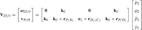
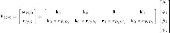

On the other hand, since each leg shares a common fixed and mobile platform, i.e., links 5, 15, 25, 35 and 45 represent the mobile platform, whereas links 0, 10, 20, 30 and 40 represent to the fixed platform, it can be stated that:
which yields the following matrix array:where:
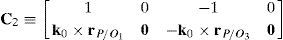
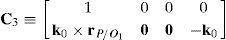


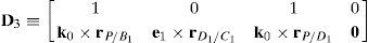
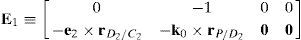

Eq. (40) will be referred to as structural velocity model. It should be noted that equation (40) does not contain any parameter (e.g., the Cartesian coordinates x˙, y˙, z˙ of velocity vector of point P) related to the output motion of the mobile platform, but it only contains input joint velocitiesq˙I and passive joint velocitiesq˙P.
5.2Velocity analysis related to the input and output motionsIn a parallel manipulator, the architecture of the legs determines the transformation of the joint motions into motions of the mobile platform. Thus, the mobile platform acquires a certain velocity state through the actuation of the legs composing the parallel manipulator. Hence the objective of this section is to relate the output motion of the mobile platform with the input motions generated by manipulator's actuators.
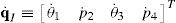
For the purposes of this paper, the output motion is defined as the velocity state of the mobile platform with respect to the fixed platform, namely, V5/0≡(ω5/0, vP/O)T. On the other hand, the input motion is defined by a four-dimensional vector q˙I, which involves the input joint velocities of the parallel manipulator, i.e., q˙I≡(θ˙1,p˙2,θ˙3,p˙4)T.
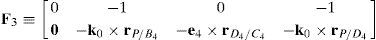
In order to reach the objective formulated previously, theory of reciprocal screws can be used to provide an elegant formulation. Thus, computing the Klein form of both sides of Eqs. (35)–(38), and after some algebra, it follows that:
where: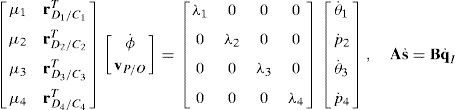
Given the role represented by Eq. (41), it will be referred to as input–output velocity model. It should be noted that Eq. (41) directly relates the output motion, vP/O, ϕ˙, with the input motion, q˙I. In other words, the output motion is decoupled from the passive joint motions, q˙P.
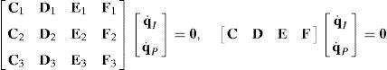
5.3Global velocity modelThe so-called global velocity model includes both, the structural velocity model (40), as well as the input-output velocity model (41). Thus, the global velocity model is constructed by assembling equations (40) and (41) in one single matrix array, which is given by:
where O4×4 and O12×4 are zero matrices, whereas 016×1 is a zero vector. It should be noted that equation (42) is an homogeneous linear system of 16 equations in 20 unknowns.6Singularity analysis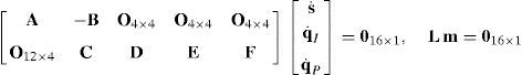
Speaking in simple words, a first order singularity analysis deals with the detection and interpretation of the different solutions of the global velocity model (42). If there can be made a choice between solutions, it may be important to consider which solutions have additional interesting properties. This is the motivation behind a singularity analysis. Thus, a singularity occurs whenever there is an instantaneous alteration of the finite mobility of the mechanism, which may be related, for example, to the blockage of the actuators or to the loss of control on the motion of some link, e.g., the mobile platform of a parallel manipulator. Moreover, each singularity type is characterized by the occurrence of a certain physical phenomenon, which results from the indeterminacy of the global velocity model. Therefore, conditions for the occurrence of singularity are presented next.
6.1Lost output motionsThere exist situations where the infinitesimal motion of the moving platform along certain directions cannot be accomplished. Hence, the manipulator loses one or more degrees of freedom. In this regard, it would be interesting to know if there exist some nonzero vectors, q˙I and q˙P, that result in a zero vector s˙. Under such circumstances, the global velocity model (42) becomes:
being LO a (16×16) square matrix.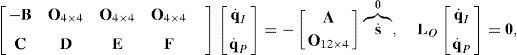
On the one hand, if matrix LO is nonsingular, all the input motions, q˙I, as well as all the passive joint rates, q˙P, become zero from the homogeneous equation (43) and, as expected, the manipulator instantaneously becomes an immobile structure. On the other hand, from linear algebra it is well-known that the homogeneous equation (43) may have non-trivial solutions when matrix LO is singular. This implies that at the configuration corresponding to loss of rank of LO or when det(LO)=0, the foregoing immobile structure may have non-zero vectors q˙I and q˙P, and therefore, the immobile structure recovers certain joint motions, but no output motion is generated.
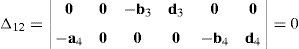
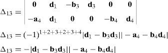
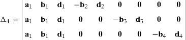
Due to the particular form of matrix LO, its determinant may be expanded by using Laplace's theorem (Crane & Duffy, 1998; Korn & Korn, 2000), thus yielding:
where:
A singularity will occur if the right hand side of equation (44) vanishes. However, this expression is the product of two additional determinants. Hence the analysis is divided into two parts, each corresponding to each of the two determinants.
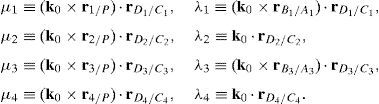
6.1.1Singularities associated with matrix −BFrom equation (41) it is apparent that:
Matrix −B is singular when the right hand side of equation (46) is equal to zero. This expression is the product of four scalar quantities. Therefore, the singularity analysis of matrix −B will be composed of four parts.
Case 1 Scalar λ1=0. Resorting to basic properties of vector triple products and, from equation (41), this condition yields:

There are three subcases depending on the relative orientation between vectors k0, rB1/A1 and rD1/C1:
- Subcase 1.1
According to the first right hand side of equation (47), this type of singular configuration is reached whenever k0, rB1/A1 and rD1/C1 are coplanar. However, position vector rD1/C1 is not necessarily parallel to unit vector k0 or position vector rB1/A1.
- Subcase 1.2
The second right hand side of equation (47) implies that link 13 is parallel to line A1B1, i.e., rB1/A1×rD1/C1=0.
- Subcase 1.3
Finally, the third right hand side of equation (47) means that link 13 is parallel to Z0 axis, i.e., rD1/C1×k0=0.
At these configurations, the motion of the corresponding actuator, namely, θ˙1, does not produce any motion of the mobile platform.
Case 2 Scalar λ2=0. From the definition of λ2, see Eq. (41), this condition leads to:
This type of singular configuration is reached when unit vector k0 is perpendicular to position vector rD2/C2, which means that link 23 is on a plane parallel to the X0Y0 plane. At this configuration, the motion of the corresponding actuator, namely, p˙2, does not contribute to the motion of the mobile platform.
Case 3 Scalar λ3=0. From the definition of λ3, see equation (41), and, after using basic properties of vector triple products, this condition leads to: Resorting to the first right hand side of equation (49), this type of singular configuration is reached whenever k0, rB3/A3 and rD3/C3 are coplanar. However, it is not necessary that position vector rD3/C3 be parallel to unit vector k0 or position vector rB3/A3. The second right hand side of equation (49) implies that link 33 is parallel to line A3B3, i.e., rB3/A3×rD3/C3=0. Finally, the third right hand side of equation (49) means that link 33 is parallel to Z0 axis, i.e., rD3/C3×k0=0.

At anyone of these configurations, the motion of the corresponding actuator, namely, θ˙3, does not produce any motion of the mobile platform.
Case 4Scalar λ4=0.
According to the definition of parameter λ4, see (41), this condition can be formulated as follows:
This singular configuration is achieved when unit vector k0 is perpendicular to position vector rD4/C4, which means that link 43 lies on a plane parallel to the X0Y0 plane. At this configuration, the motion of the corresponding actuator, namely, p˙4, does not contribute to the motion of the mobile platform.
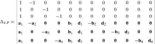
6.1.2Singularities associated with matrix LPIn order to perform a comprehensive and exhaustive analysis of the singularities related to matrix LP, it is proposed an integrated approach composed of two focuses. On the one hand, the singularity is related to the loss of rank of matrix LP. Although the exhaustiveness of this focus may be difficult to achieve, the corresponding mathematical process is relatively easy to be conducted. On the other hand, the singularity of matrix LP may be also directly related to the symbolic expression of its determinant, i.e., det(LP). However, since LP is a 12×12 matrix, the symbolic computation of its determinant is a real challenge, as it is shown in Appendix A. No matter which approach is used, both focuses produce results with physical insight, and they are complementary one of the another.
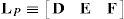
Firstly, analyzing the form of equation (45), matrix LP can be written as follows:
where:
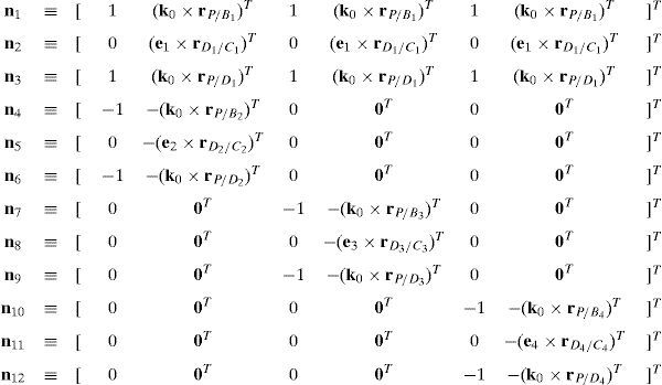
Matrix LP is singular when: (a) it becomes rank-deficient, that is, when some of its columns are linearly dependent, or, equivalently, (b) its determinant is zero, that is, det(LP)≡ΔLP=0. In what follows, a complete description of linearly dependent sets of columns is introduced. Moreover, in order to form a satisfactory and balanced whole, each case is also associated with the symbolic expression of ΔLP, which is shown in Appendix A.Case 1 Columns n1 and n3 are linearly dependent. Columns n1 and n3 are linearly dependent when there exist two scalars ϵ1, ϵ2, both different from zero, such that:


On the other hand, speaking now in terms of the determinant ΔLP, see Eq. (A.47) appearing in Appendix A, this particular case of singularity is represented by the vector product:

Thus, when condition (55) is satisfied, the right hand side of equation (56) becomes zero vector, i.e., b1×d1=0 and, therefore, ΔLP=0.
Case 2Columns n4 and n6 are linearly dependent.
The set of columns n4 and n6 is linearly dependent if it is possible to find two scalars, ¿1≠0, ¿2≠0, which satisfy the following relation:
a condition that leads to:equation whose solution is given by:as it is graphically illustrated in Figure 9. For this particular type of singularity, the motion axes of angles φ2 and γ2, which are shown in Figure 4, are coaxial. Moreover, from the geometry shown in Figure 9, it can be concluded that, for this type of singularity, link 23 is parallel to axis Z0, that is, vectors rD2/C2 and k0 are parallel.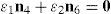


Now, if we resort to the mathematical form of the determinant ΔLP, see Appendix A, this particular case of singularity is represented by the vector product:

Thus, when condition (60) is satisfied, the right hand side of equation (61) becomes zero vector, i.e., b2×d2=0 and, therefore, ΔLP=0. It should be noted that vector product b2×d2 appears in all the components of the first factor of the right hand side of equation (A.47), see Appendix A.
Case 3Columns n7 and n9 are linearly dependent.
The set of columns n7 and n9 is linearly dependent when there exist two scalars ς1, ς2, both different from zero, such that:
which implies that:equation whose solution is given by:as it is graphically illustrated in Figure 9. For this particular type of singularity, the motion axes of angles φ3 and γ3, which are shown in Figure 5, are coaxial. Moreover, from the geometry shown in Figure 9, it can be concluded that, for this type of singularity, link 33 is parallel to axis Z0, that is, vectors rD3/C3 and k0 are parallel.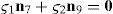


On the other hand, resorting to the mathematical form of the determinant ΔLP, see Appendix A, this particular case of singularity is represented by the vector product:

Thus, when condition (65) is satisfied, the right hand side of equation (66) becomes zero vector, i.e., b3×d3=0 and, therefore, ΔLP=0. It should be noted that vector product b3×d3 appears in all the components of the first factor of the right hand side of equation (A.47), see Appendix A.
Case 4Columns c10 and c12 are linearly dependent.
This case deals with the possibility to find two scalars, ξ1≠0, ξ2≠0, which satisfy the following relation:
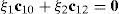
Thus, if relationship (67) is satisfied, then the set of columns c10 and c12 constitutes a linearly dependent. Furthermore, such a condition leads to:
equation whose solution is given by:as it is graphically illustrated in Figure 9. For this particular type of singularity, the motion axes of angles φ4 and γ4, which are shown in Figure 6, are coaxial. Moreover, Figure 9 reveals that, at the singularity at hand, link 43 is parallel to axis Z0, that is, vectors rD4/C4 and k0 are parallel.


Now, analyzing the mathematical form adopted by the determinant ΔLP, see Appendix A, this particular case of singularity is represented by the vector product:

Thus, when condition (70) is satisfied, the right hand side of equation (71) becomes zero vector, i.e., b4×d4=0 and, therefore, ΔLP=0. It should be noted that vector product b4×d4 appears in all the components of the first factor of the right hand side of equation (A.47), see Appendix A.
Case 5Columns n2, n5, n8 and n11 are linearly dependent.
The main objective related to this particular case may be formulated in terms of the possibility to find four scalars, η1≠0, η2≠0, η3≠0, η4≠0, which satisfy the following relation:

When condition (72) is fulfilled, then columns n2, n5, n8 and n11 constitute a linearly dependent set. Moreover, resorting to equation (51) and analyzing the particular form of vectors n2, n5, n8 and n11, it can be concluded that condition (72) leads to the following vector equations:
equations whose common solution is given by:which means that links 13, 23, 33, and 43 are parallel and, the motion axes of joint angles β1, β2, β3, and β4 are parallel too.


On the other hand, determinant ΔLP can be written as follows:
where k2≡(b2×d2)·(a2−a1), k3≡(b3×d3)·(a3−a1), k4≡(b4×d4)·(a4−a1) and bi≡ei×rDi/Ci, for i=1, 2, 3, 4.
Thus, when condition (76) is satisfied, it means that b1=b2, b1=b3 and b1=b4. In consequence, the right hand side of equation (77) becomes zero since, for i=2, 3, 4, and j=3, 4, 2, respectively:
where bi·(bj×dj)=0 and b1·(d1×bj)=0 for i=2, 3, 4, and j=3, 4, 2, respectively. As a result, ΔLP=0.6.2Locked actuated joints
Another important physical phenomenon related to singularity analysis occurs when all the actuated joints are locked. This fact implies that vector q˙I must be set to zero. Thus, the mobile platform may possess infinitesimal motion in some directions while all the actuators are completely locked. For this particular case, the global velocity model (42) becomes:
where LI is a (16×16) square matrix.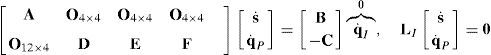
Then, if matrix LI is nonsingular, all the output motions, s˙, as well as all the passive joint rates, q˙P, become zero from equation (79) and, as expected, the manipulator becomes an immobile structure. On the other hand, from linear algebra it is well-known that homogeneous equation (79) may have non-trivial solutions when matrix LI is singular. This implies that at the configuration corresponding to loss of rank of LI or when det(LI)=0, the foregoing immobile structure may have non-zero vectors s˙ and q˙P, and thereby the manipulator gains one or more degrees of freedom. It is important to remark that this type of singularity is particularly dangerous since the gained degrees of freedom are unexpected. Therefore, serious damages to people or surrounding equipment may result.
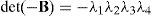
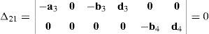
Analyzing the form of matrix LI, it may be observed that submatrix A has three zero submatrices O4×4 on the right and a zero submatrix O12×4 behind it. This particular form can be exploited in order to obtain the determinant of matrix LI. Hence, its determinant may be expanded by using Laplace's theorem (Crane & Duffy, 1998; Korn & Korn, 2000), thus yielding:

A singularity will occur if the right hand side of equation (80) vanishes. However, this expression is the product of two additional determinants. Hence the analysis is divided into two parts, each corresponding to each of the two determinants.
6.2.1Singularities associated with matrix AThe determinant of matrix A, see equation (41), can be computed by the expansion of its first column, that is:
where:
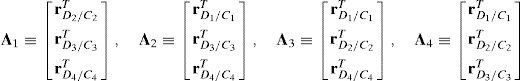
Matrix A is singular when the right hand side of equation (81) is equal to zero. This expression is composed of four different scalar quantities. Therefore, several singularities are identified next.Case 1 Scalars μ1=0, μ2=0, μ3=0 and μ4=0. In order to present a systematic formulation of this particular case of singularity, the following approach is proposed. Firstly, from the definition of parameters μ1, μ2, μ3 and μ4 and, after using basic properties of triple vector products:


On the one hand, satisfaction of condition (82) leads to the identification of three subcases:
- Subcase 1.1
According to the first right hand side of equation (82), this type of singular configuration is reached whenever k0, r1/P and rD1/C1 are coplanar. However, position vector rD1/C1 is not necessarily parallel to unit vector k0 or position vector r1/P.
- Subcase 1.2
The second right hand side of equation (82) implies that link 13 is parallel to a line going from point P to point 1, i.e., r1/P×rD1/C1=0.
- Subcase 1.3
Finally, the third right hand side of equation (82) means that link 13 is parallel to Z0 axis, i.e., rD1/C1×k0=0.
On the other hand, condition (83) is satisfied when:
- Subcase 1.4
According to the first right hand side of equation (83), this type of singular configuration is reached whenever k0, r2/P and rD2/C2 are coplanar. However, position vector rD2/C2 is not necessarily parallel to unit vector k0 or position vector r2/P.
- Subcase 1.5
The second right hand side of equation (83) implies that link 23 is parallel to a line passing through points 2 and P, i.e., r2/P×rD2/C2=0.
- Subcase 1.6
Finally, the third right hand side of equation (83) means that link 23 is parallel to Z0 axis, i.e., rD2/C2×k0=0.
In turn, condition (84) is satisfied when:
- Subcase 1.7
According to the first right hand side of equation (84), this type of singular configuration is reached whenever k0, r3/P and rD3/C3 are coplanar. However, position vector rD3/C3 is not necessarily parallel to unit vector k0 or position vector r3/P.
- Subcase 1.8
The second right hand side of equation (84) implies that link 33 is parallel to a line that includes point 3 and point P, i.e., r3/P×rD3/C3=0.
- Subcase 1.9
Finally, the third right hand side of equation (84) means that link 33 is parallel to Z0 axis, i.e., rD3/C3×k0=0.
Additionally, satisfaction of condition (85) leads to:
- Subcase 1.10
According to the first right hand side of equation (85), this type of singular configuration is reached whenever k0, r4/P and rD4/C4 are coplanar. However, position vector rD4/C4 is not necessarily parallel to unit vector k0 or position vector r4/P.
- Subcase 1.11
The second right hand side of equation (85) implies that link 43 is parallel to line 4−P, i.e., r4/P×rD4/C4=0.
- Subcase 1.12
Finally, the third right hand side of equation (85) means that link 43 is parallel to Z0 axis, i.e., rD4/C4×k0=0.
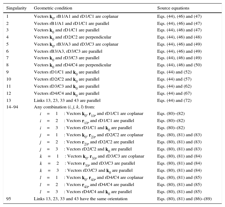
It should be noted that the singularity under analysis is reached only when all the scalars μ1, μ2, μ3, and μ4, are simultaneously equal to zero. Hence it is necessary to detect all the feasible combinations of subcases shown previously. Thus, such a procedure leads to the identification of 81 different singularities shown in Table 1, namely, singularities 14 to 94.
Singularities of the Schönflies parallel manipulator.
| Singularity | Geometric condition | Source equations |
|---|---|---|
| 1 | Vectors k0, rB1/A1 and rD1/C1 are coplanar | Eqs. (44), (46) and (47) |
| 2 | Vectors rB1/A1 and rD1/C1 are parallel | Eqs. (44), (46) and (47) |
| 3 | Vectors k0 and rD1/C1 are parallel | Eqs. (44), (46) and (47) |
| 4 | Vectors k0 and rD2/C2 are perpendicular | Eqs. (44), (46) and (48) |
| 5 | Vectors k0, rB3/A3 and rD3/C3 are coplanar | Eqs. (44), (46) and (49) |
| 6 | Vectors rB3/A3, rD3/C3 are parallel | Eqs. (44), (46) and (49) |
| 7 | Vectors k0 and rD3/C3 are parallel | Eqs. (44), (46) and (49) |
| 8 | Vectors k0 and rD4/C4 are perpendicular | Eqs. (44), (46) and (50) |
| 9 | Vectors rD1/C1 and k0 are parallel | Eqs. (44) and (52) |
| 10 | Vectors rD2/C2 and k0 are parallel | Eqs. (44) and (57) |
| 11 | Vectors rD3/C3 and k0 are parallel | Eqs. (44) and (62) |
| 12 | Vectors rD4/C4 and k0 are parallel | Eqs. (44) and (67) |
| 13 | Links 13, 23, 33 and 43 are parallel | Eqs. (44) and (72) |
| 14–94 | Any combination (i, j, k, l) from: | |
| i=1: Vectors k0, r1/P and rD1/C1 are coplanar | Eqs. (80)–(82) | |
| i=2: Vectors r1/P and rD1/C1 are parallel | Eqs. (80)–(82) | |
| i=3: Vectors rD1/C1 and k0 are parallel | Eqs. (80)–(82) | |
| j=1: Vectors k0, r2/P and rD2/C2 are coplanar | Eqs. (80), (81) and (83) | |
| j=2: Vectors r2/P and rD2/C2 are parallel | Eqs. (80), (81) and (83) | |
| j=3: Vectors rD2/C2 and k0 are parallel | Eqs. (80), (81) and (83) | |
| k=1: Vectors k0, r3/P and rD3/C3 are coplanar | Eqs. (80), (81) and (84) | |
| k=2: Vectors r3/P and rD3/C3 are parallel | Eqs. (80), (81) and (84) | |
| k=3: Vectors rD3/C3 and k0 are parallel | Eqs. (80), (81) and (84) | |
| l=1: Vectors k0, r4/P and rD4/C4 are coplanar | Eqs. (80), (81) and (85) | |
| l=2: Vectors r4/P and rD4/C4 are parallel | Eqs. (80), (81) and (85) | |
| l=3: Vectors rD4/C4 and k0 are parallel | Eqs. (80), (81) and (85) | |
| 95 | Links 13, 23, 33 and 43 have the same orientation | Eqs. (80), (81) and (86)–(89) |
Determinants of matrices A1, A2, A3, and A4 are zero.
Since the determinants of matrices A1, A2, A3 and A4 can be written in terms of triple vector products (Brand, 1947; Hao & McCarthy, 1998) then this type of singularity can be formulated as follows:
which are expressions that can be simultaneously satisfied when all the involved position vectors are parallel, that is, rD1/C1∥rD2/C2, rD1/C1∥rD3/C3 and rD1/C1∥rD4/C4. Speaking in practical terms, at this configuration, links 13, 23, 33 and 43 must have the same orientation. This is the singularity number 95, which has been included in Table 1.


It is important to point out that, a careful analysis of the singularities shown in Table 1 reveals that singularities 13 and 95 are very similar. However, it should be noted that singularity 13 is related to lost output motions, whereas singularity 95 arose from the analysis of the locked actuated joints. This is the reason because of both singularities were included separately.
Finally, in order to satisfy condition (80), det(LP)=0. However, it should be recalled that singularities associated with matrix LP were previously analyzed and discussed in Section 6.1.2. Therefore, the singularity analysis has been completed.
In summary, all the singularities that were detected and discussed in the previous subsections are now shown in Table 1.
From Table 1, a total of 95 different singularities were detected for the Schönflies manipulator under analysis.
7Singularity plotsIn order to have a more detailed idea about the distribution of the singularities throughout the workspace, several singularity plots were graphically generated. On the one hand, Figures 10–19 are singularity plots corresponding to those geometrical dimensions of the manipulator that were used early in the workspace generation.
 manipulator")
 manipulator")
 manipulator")
 manipulator")
 manipulator")
 manipulator")
 manipulator")
 manipulator")
 manipulator")
 manipulator")
On the other hand, in order to obtain more singularity configurations of the manipulator, the fixed platform was geometrically modified. As a result, a set of different geometrical dimensions for:
- (a)
Figure 20, were taken as R1X=113.89, R2X=42.34, R2Y=254.92, R3X=−211.92, R3Y=15.55, R4X=55.67, R4Y=−270.48, and constant angles α2=1.45∘, α3=0∘ and α4=1.45∘,
- (b)
Figure 21, are R1X=98.75, R2X=−127.84, R2Y=189.13, R3X=−61.79, R3Y=−92.33, R4X=90.89, R4Y=−96.79, and constant angles α2=37.41∘, α3=0∘ and α4=37.41∘,
- (c)
Figure 22, were selected as R1X=163.55, R2X=1.61, R2Y=275.24, R3X=−161.72, R3Y=4.68, R4X=−3.44, R4Y=−279.92, and constant angles α2=0.52∘, α3=0∘ and α4=0.52∘, and,
- (d)
Figure 23, are given by R1X=215.50, R2X=10.10, R2Y=167.85, R3X=−216.36, R3Y=23.59, R4X=−9.24, R4Y=−191.44, and constant angles α2=6.46∘, α3=0∘ and α4=6.46∘.
: (a) manipulator")
: (a) manipulator")
: (a) manipulator")
: (a) manipulator")
A detailed singularity and workspace analyses of a particular Schönflies parallel manipulator have been presented in this paper. As a result, a total of 95 different types of singularities were detected. Moreover, geometrical conditions that characterize each type of singularity were explained and mathematically formulated. It is expected that both analyses should be useful to avoid dangerous configurations of the manipulator during the stage of trajectory planning.
Conflict of interestThe authors have no conflicts of interest to declare.
The authors acknowledge the support of the Consejo Nacional de Ciencia y Tecnología (National Council of Science and Technology, CONACYT), of México, through SNI (National Network of Researchers) fellowships and scholarships.
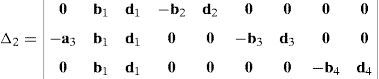
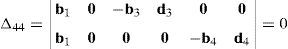
The objective of this appendix is to show all the details involved into the symbolic computation of the determinant of matrix LP, which is given by Eq. (51).
The procedure begins by adopting the following definitions:


Thus, the determinant ΔLP of matrix LP, see equation (51), is given by:
Interchange of the ninth row to the second row and the fifth row to the third row leads to:
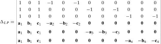
Subtracting the first column from the third column, the fourth column from the sixth column, the seventh column from the ninth column and the tenth column from the twelfth column:
where: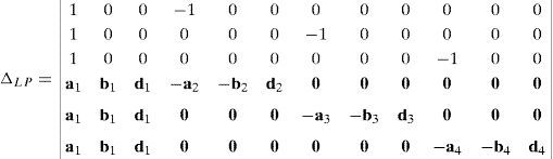

Next, after interchanging column 4 to column 2, column 7 to column 3 and column 10 to column 4, determinant ΔLP becomes:
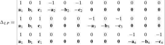
Now, Laplace's theorem may be applied to evaluate determinant ΔLP by forming the product of every 3×3 determinant from the first three rows of ΔLP times its corresponding 9×9 complement determinant. Determinant ΔLP can thus be evaluated as:
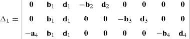
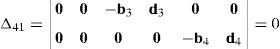
where each sub-determinant Δ1, Δ2, Δ3 and Δ4 will be evaluated separately.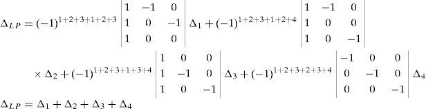

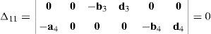


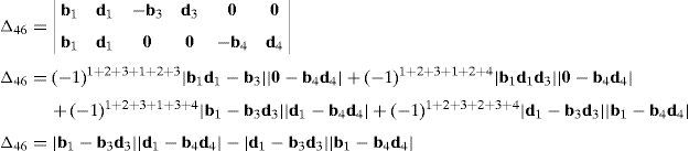
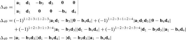
The third determinant Δ3 is given by:
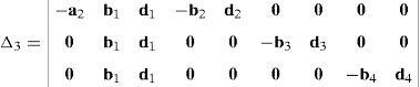
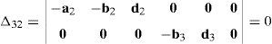
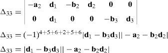
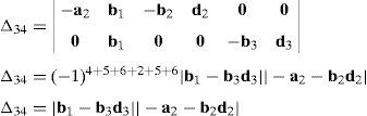
Resorting to Laplace's theorem, determinant Δ3 may be evaluated by forming the product of every 3×3 determinant from the last three rows of Δ3 times its corresponding 6×6 complement determinant, which yields:
where, in turn:thus, the following result is finally obtained:


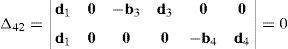
The last determinant Δ4 is mathematically given by:
Similarly, according to Laplace's theorem, determinant Δ4 may be evaluated by forming the product of every 3×3 determinant from the first three rows of Δ4 times its corresponding 6×6 complement determinant, which yields:
where the involved determinants are given by: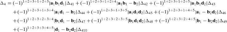


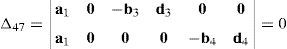
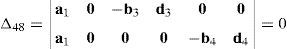
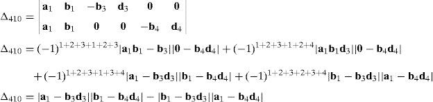
Thus, after regrouping all the terms involved into equation (A.33) it is obtained that:

On the other hand, expanding and regrouping the elements of equation (A.10) and recognizing (Schwartz, Green, & Rutledge, 1964) that:
it is finally obtained that:which is the result sought.


According to the approach proposed in the manipulator under study was obtained by assembling four legs. These four legs include two types of basic legs proposed in Kong and Gosselin (2007), which were designed to generate a Schönflies motion. However, it is important to mention that this particular manipulator, as a whole, is not explicitly reported in Kong and Gosselin (2007).
Peer Review under the responsibility of Universidad Nacional Autónoma de México.
The velocity state of body i with respect to body j is denoted by Vi/j≡(ωi/j,vPi/Oj)T. This is a six-dimensional vector composed of two three-dimensional vectors: (a) the angular velocity vector of body i with respect to body j, namely, ωi/j, and (b) the velocity vector vPi/Oj of a point Pi (fixed on body i) with respect to any point of body j, such as point Oj.