


In this paper we present a new approach to design the input control to track the output of a non-minimum phase nonlinear system. Therefore, a cascade control scheme that combines input–output feedback linearization and gradient descent control method is proposed. Therein, input–output feedback linearization forms the inner loop that compensates the nonlinearities in the input–output behavior, and gradient descent control forms the outer loop that is used to stabilize the internal dynamics. Exponential stability of the cascade-control scheme is provided using singular perturbation theory. Finally, numerical simulation results are presented to illustrate the effectiveness of the proposed cascade control scheme.
vector of state variables
control input
output variable
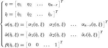
vector of slow state variables
vector of fast state variables of the internal dynamics
local minimal point of an control variable u
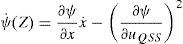
scalar output
reference trajectory for the output
state vector of reduced subsystem
virtual desired output
QSS control input
artificial input
Lyapunov function
performance function of an control variable u
descent function
The control of nonlinear non-minimum phase systems is a challenging problem in control theory and has been an active research area for the last few decades. This technique, as a matter of fact, was successfully established in various practical applications (Bahrami, Ebrahimi, & Asadi, 2013; Cannon, Bacic, & Kouvaritakis, 2006; Charfeddine, Jouili, Jerbi, & Benhadj Braiek, 2010; Jouili & BenHadj, 2015; Sun, Li, Gao, Yang, & Zhao, 2016). This system control is a delicate task owing to the fact that it is a nonlinear system with non-minimum phase, and that it is also characterized by a dynamic prone to the instability of the dynamics of zero (Jouili & Jerbi, 2009; Jouili, Jerbi, & Benhadj Braiek, 2010; Kazantzis, 2004; Naiborhu, Firman, & Mu’tamar, 2013). In fact there exist no generic methods for controller synthesis and design (Khalil, 2002). Several fundamental methods in the output tracking problems on nonlinear non-minimum phase systems have been proposed in this area.
Hirschorn and Davis (1998), Isidori (1995), and Hu et al. (2015) have proposed the stable inversion method to the tracking problem with unstable zero dynamics. This method tries to find a stable solution for the full state space trajectory by steering from the unstable zero dynamics manifold to the stable zero dynamics manifold.
Khalil (2002) has derived a minimum phase approximation to a single-input single-output nonlinear, non-minimum phase system. An input–output linearizing controller is designed for this approximation and then applied to the non-minimum phase plant. This leads to a system that is internally stable. Naiborhu and Shimizu (2000) presented a controller designed based upon an internal equilibrium manifold where this controller pushes the state of a nonlinear non-minimum phase system toward that manifold. This has afforded approximate output tracking for nonlinear non-minimum phase systems while maintaining internal stability.
Kravaris and Soroush have developed several results on the approximate linearization of non minimum phase systems (Kanter, Soroush, & Seider, 2001; Kravaris & Daoutidis, 1992; Kravaris, Daoutidis, & Wright, 1994; Soroush & Kravaris, 1996). For instance Kanter et al. (2001) and Kravaris et al. (1994) investigated the system output which is differentiated as many times as the order of the system where the input derivatives that appear in the control law are set to zero when computing the state feedback input. Bortoff (1997) has studied the system input–output feedback of the first linearized. Then, the zero dynamics is factorized into stable and unstable parts. The unstable part is approximately linear and independent of the coordinates of the stable part. Charfeddine, Jouili, and Benhadj Braiek (2015) dismissed a part of the system dynamics in order to make the approximate system input-state feedback linearizable. The neglected part is then considered as a perturbation part that vanishes at the origin. Next, a linear controller is designed to control the approximate system.
Moreover, an original technique of control based on an approximation of the method of exact input–output linearization, was proposed in the works (Charfeddine, Jouili, Jerbi, & Benhadj Braiek, 2011; Guardabassi & Savaresi, 2001; Guemghar, Srinivasan, Mullhaupt, & Bonvin, 2002; Hauser, Sastry, & Kokotovic, 1992). The approximation (Charfeddine et al., 2011) is used to improve the desired control performance. A cascade control scheme has been considered (Charfeddine, Jouili, & Benhadj Braiek, 2014; Yakoub, Charfeddine, Jouili, & Benhadj Braiek, 2013) that combines the input–output feedback linearization and the backstepping approach.
On the other hand, Firman, Naiborhu, and Saragih (2015) have applied the modified steepest descent control for that system output will be redefined such that the system becomes minimum phase with respect to a new output.
In this paper, we address the problem of tracking control of a single-input single-output of non-minimum phase nonlinear systems. The idea here is to transform the given system into Byrnes–Isidori normal form, then to use the singular perturbed theory in which a time-scale separation is artificially introduced through the use of a state feedback with a high-gain for the linearized part. The gradient descent control method (Naiborhu & Shimizu, 2000) is introduced to generate a reference trajectory for stabilizing the internal dynamics.
This results in a cascade control scheme, where the outer loop consists of a gradient descent control of the internal dynamics, and the inner loop is the input–output feedback linearization.
The stability analysis of the cascade control scheme is provided using results of singular-perturbation theory (Khalil, 2002).
The rest of this paper is organized as follows. In Section 2, some mathematical preliminaries are presented. The proposed cascade control scheme and the stability analysis are given in Sections 3 and 4, respectively. In Section 5, the effectiveness of the proposed control scheme is illustrated by numerical examples. Finally, this paper will be closed by a conclusion and a future works presentation.
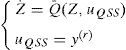
2Theoretical backgroundIn this paper, we consider a single-input single-output nonlinear system of the form:
where x∈ℜn is the n-dimensional state variables, u∈ℜ is a scalar manipulate input and y∈ℜ is a scalar output. f(·), g(·) and h(·) are smooth functions describing the system dynamics.2.1Exact input–output feedback linearization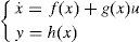
The input output linearization is based on two concepts: the concept of relative degree and the concept of state transformation.
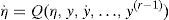
The relative degree r of the system (1) is defined as the number of derivation of the output y needed to appear in the input u, such as ∀x∈ℜn:
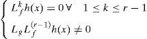
If r≤n, then system (1) can be feedback linearized into Byrnes–Isidori normal form (Isidori, 1995) using the following steps:
Step 1: We apply the following control law
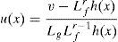
This control law compensates the nonlinearities in the input–output behavior.
Step 2: First, system (1) is transformed into normal form (Isidori, 1995) through a nonlinear change of coordinates:
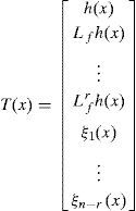

The resulting system with the transformed variables (4) can then be written as
where η is the state vector of the internal dynamics.2.2Singular perturbed system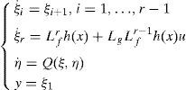
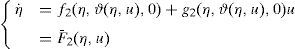
A singularly perturbed system is a system that exhibits a two-time scale behavior, i.e. it has slow and fast dynamics, and it is modeled as follows (Glielmo & Corless, 2010):
where ξ∈ℜP and η∈ℜm are respectively the slow and fast variables and ¿>0 is a small positive parameter. The functions F1(·) and F2(·) are assumed to be continuously differentiable.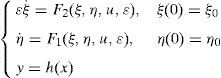
ξ0 and η0 are respectively the initial conditions of the vectors ξ and η. If ¿→0, the dynamics of ξ acts quickly and leads to a time-scale separation. Such a separation can either represent the physics of the system or can be artificially created by the use of high-gain controllers.
As ¿→0, ξ can be approximated by its Quasi Steady State ξ¯=ϑ(η,u) obtained by solving

So, the reduced (slow) system is given by:
Note that the reduced system (8) is not necessarily affine in input.
In the next theorem, we establish the exponential stability of the singular perturbed system (7).Theorem 1Khalil, 2002 Assume that the following conditions are satisfied: The origin is an equilibrium point for (7), ϑ(η, u) has a unique solution, The functions f1, f2, g1, g2, ϑ and their partial derivatives up to order 2 are bounded for ξ in the neighborhood of ξ¯, The origin of the boundary-layer system (7) is exponentially stable for all η, The origin of the reduced system (9) is exponentially stable.
Then, there exists ¿∗>0 such that, for all ¿<¿∗, the origin of (7) is exponentially stable.Theorem 2Khalil, 2002 Given system (1), if there exists a Lyapunov function V(x) and positive constants χ1, χ2 and χ3 such that χ1x2≤V(x)≤χ2x2 and V˙(x)≤−χ3x2, then the origin is exponentially stable.
The trajectory following method (Naiborhu & Shimizu, 2000) is a numerical optimization method based on solving continuous differential equations.
The basic idea behind a “trajectory following” method is to form a set of differential equations from the gradient of the cost function.
Consider first the minimizing problem of the form:
where ϒ(u) is a performance function of a control variable u.

Suppose that we use the local minimal point u* as an initial condition for integrating the differential equation,
where Λ(·) is a function at our disposal, to be determined shortly.
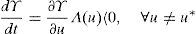
Calculate the time derivative of ϒ(u) along the trajectory generated by the solution to (11). Then at u=u*:
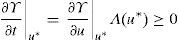
Since we are interested in a trajectory that will search a minimum, the above observation suggests that we integrate (11) by choosing
and Eq. (12) becomes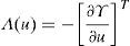
Thus, in order to solve the problem of minimizing ϒ(·) in an unconstrained control space, one need only to choose an appropriate initial condition for u and integrate
until the equilibrium solution is achieved.3Synthesis of the proposed control scheme
In this section, a cascade control scheme for the tracking control problem of nonlinear non-minimum phase systems is proposed. The idea of the control scheme is to use the input–output feedback linearization in the inner loop and the gradient descent control in the outer loop. The input–output feedback linearization can be seen as a pre-compensator prior to applying gradient descent control, whereas gradient descent control can be viewed as a systematic way of controlling the internal dynamics. The following control structure is proposed (Fig. 1).

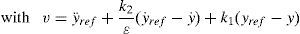
Consider the nonlinear system described by (1), then we apply the control law (3) which is given by:
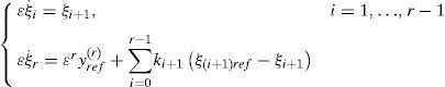
where yref is the reference trajectory for the output, ¿→0 a small positive parameter, and ki>0, ∀i∈{1, 2, …, n−1} are the coefficients of a Hurwitz polynomial (Isidori, 1995) and the internal dynamics are given by: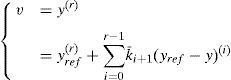
Under the assumption that the gains k¯i are chosen large, such as for any choice of ¿>0, the closed loop is stable and ¿ can be used as a single tuning parameter, the system (16) and (17) can be written in the form of a singular perturbed system (7). So the fast state can be defined by:

If we replace (18) by (17), we obtain
and also by (16), such thatthus, (17) can be written as follows:3.2Reduced subsystem
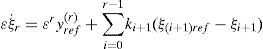

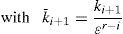
The internal dynamics depends on the output y and its derivatives y˙,…,y(r−1), such as:
In general, the input output linearization techniques decouple between the input–output behavior y and the internal dynamics η. On the other hand, the QSS assumption decouples between the internal dynamics η and the input output behavior y. Thus, y does not have any effect on η. Therefore, the output y(r) is used for the control of the internal dynamics. Thus, the boundary layer subsystem (21) and the reduced subsystem (22) can be manipulated separately.
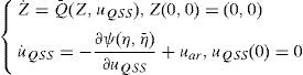
Firstly, we define a novel state vector:
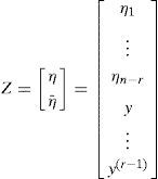
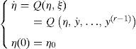
Such as the reduced subsystem (22) can be written by:
The system (24) will be expressed by the following state equation:
where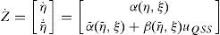
The stability of the internal state η is required to guarantee the output system y tracks the reference output trajectory yref. Based on the gradient descent control algorithm, we propose a method to make the internal state η tend to ηref, η→ηref if t→∞ (internal state regulation).
Let η be a virtual output of the system and ηref be the virtual desired output.
Then we find γη as relative degree of the system if η is the output of the system (1). We know that η∈R(n−r) then γη=γη1γη2…γη(n−r). Based on Z and their derivatives, we construct the performance index as a descent function as follows
where the constants a0,a1…,ar,b0i,b1i,…,bγii,i=1,…,(n−r) will be chosen later.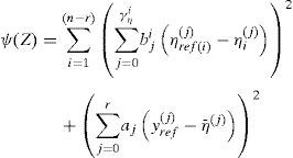
Reasons why we define the descent function as in (26) are:
- i.
The input uQSS can be designed if there exists an explicit relationship between the input uQSS and the output y. Thus, descent function (26) must be a function of ηγη1,…,ηγη(n−r),y,…,y(r−1).
- ii.
We need that the descent function:
be a quadratic form and that ψ(0) be equal to zero. Accordingly, the minimum value of the descent function ψ0(Z) is zero.

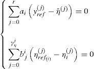
If ψ(Z) is zero, each term in the right side of Eq. (26) is positive ∀t, therefore we have:
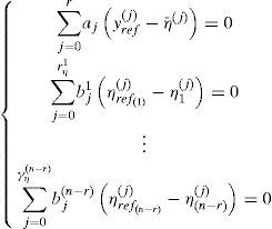
By choosing the values of a0, a1…, ar such that the Eigen values of the polynomial
are real negative and the values of b0i,b1i,…,bγii, i=1,…,(n−r) such that the Eigen values of the polynomialare real negative, we obtain that:if t→∞.


In other words output tracking and regulation of internal state are achieved together (Artstein, 1983). Our objective is to find a control law uQSS such that the descent function ψ(Z) becomes minimum. Then the output tracking problem can be written as:
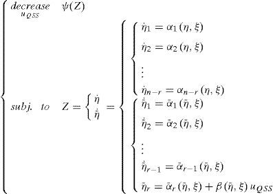
In this paper, the output tracking problem (32) will be solved using the trajectory following method.
When uQSS is a scalar,
Because the relative degree of the system is well defined,
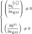
The necessary condition for a local minimum
is satisfied if at the same time:and it happens if the value of performance index ψ(Z)=0.
In the following we use a numerical technique to solve the minimization problem (32) and (33) at every point of a trajectory.
The idea of the trajectory following method is to solve the numerical optimization problem only once, at the initial point of the trajectory.
For all other points x along a trajectory, the control uQSS is determined from the differential equation:
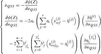
The control law in Eq. (37) is called the steepest descent control.
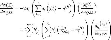
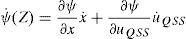
Calculate the time derivative of descent function (26)
we have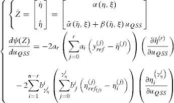
By substituting (21) into (38), we have
From Eq. (40) we see that the value of time derivative of descent function along the trajectory of (38) cannot be guaranteed to be less than zero for t≥0. Consider the extended system (38) and time derivative of descent function (40). We do not have a variable which can be used to push the time derivative of descent function (40) less than zero.
Now we modify the steepest descent control (38) by adding an artificial input uar. Then the extended system (38) becomes:
from Sontag's formula (Sontag, 1989), we get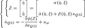
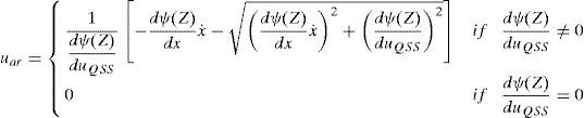
The control law in Eq. (42) is called a modified steepest descent control. A similar method using artificial input can be seen in Shimizu, Otsuka, and Naiborhu (1999).
4Stability analysisIn this section, we use Theorem 2 of exponential stability of singular perturbed system to analyze the stability of the closed loop system. If both the reduced and the boundary layer subsystems are exponentially stable, then the combination is also exponentially stable. The following steps will be used to prove the stability of the proposed approach.
4.1Exponential stability of the boundary layer subsystemLet us consider the error vector given by

Then, the boundary layer subsystem (21) becomes:
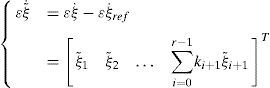
Letting τ=t/¿ yields:
with A is defined by
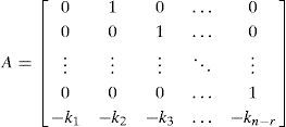
Using the Theorem 2, the origin ξ˜=0 is exponentially stable, and the Lyapunov function is
where ATP+PA=−Q and Q is a matrix defined positive.4.2Exponential stability of the reduced subsystem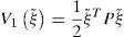
To analyze the stability of the reduced subsystem, we use the following proposition:Proposition 1 If the following statements are satisfied: The system(25)is stabilizable via the choice of uQSS (Z=0, uQSS=0) corresponds to an equilibrium point ifdψ(Z)duQSS=0
Assume that system (25) satisfies the following assumption.Assumption 1 There exists a function V2:ℜn→ℜ, V2(0)=0, which is continuous, positive definite and radially unbounded such that the unforced dynamic system of (25), namely Z˙=Q¯(Z,0) is globally asymptotically stable, i.e., V˙2(Z,uQSS)<0, Z≠0. First we define the performance index

Consider (47). If uQSS=0 then ψ(Z, uQSS)=V2(Z). In other words performance index becomes Lyapunov function and so we do not need to design control input uQSS for only stabilizing system.
With uQSS=0 we can do nothing to increase the rate of convergence. However, by adding uQSS to the system, we have freedom to accelerate the rate of convergence.
Remark 2It would appear that when Z=0 is globally asymptotically stable as assumed by Assumption 1, the global stabilization of the whole system should not be difficult.
4.3Global stabilityIn order to illustrate the stability of the cascade control scheme, the following exponential stability theorem is introduced.Theorem 3 For system(1), consider a controller where uQSSis obtained by solving the optimization problem(41)and the input is computed using(3). If P and R are positive definite, then there exists ¿>0 that would exponentially stabilize(1). UsingTheorem 1, we can conclude that there exists ¿*>0 such that for all ¿<¿*, the origin of(1)is exponentially stable. All the conditions of theorem 1 are satisfied such that: The origin((ξ=0),((η,η¯)=(0,0)))and uQSS=0 is an equilibrium point for the subsystems(21) and (25). The boundary layer subsystem(21)resulting from the QSS assumption ¿=0 has a unique solution yref. Also, as a result of the trajectory following method control, uQSSis a function of Z. The origin of the boundary layer system(21)is exponentially stable ∀Z. The origin of the reduced system(25)is exponentially stable.
In this section, we will give two illustrative examples to show the applicability and efficiency of the proposed cascade control scheme. The first example is an inverted cart-pendulum system and the second one is a ball and beam system. Controlling both systems has practical importance.
5.1Inverted cart-pendulum systemConsider the familiar inverted cart-pendulum system (Al-hiddabi, 2005), depicted in Figure 2. The cart must be moved using the force u so that the pendulum remains in the upright position as the cart tracks varying positions at the desired time. The differential equations describing the motion are (Al-hiddabi, 2005):
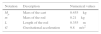
where θ is the angle of the pendulum, yp is the displacement of the cart, and u is the control force, parallel to the rail, applied to the cart. The numerical parameters of the inverted pendulum system are given in Table 1.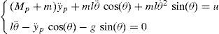

Consider yp as the output and let x=θθ˙ypy˙pT. The inverted cart-pendulum can be written as the system (1). Where yp represents the output, u is the input, x is the state-space vector. Hence, one has:
and h(x)=yp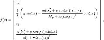
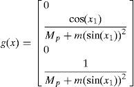
The relative degree of the system is equal to r=2 which is strictly lower than the system dimension n=4.
Applying the procedure of input–output linearization to the system (49) of the inverted cart-pendulum, the boundary layer system is given by:
its control is given by:and the internal dynamics is given by

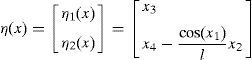
Under the QSS assumption that θ˙=θ¨=v=0 and θ→≅0, sin(θ)=θ and cos(θ)=1. Using Eq. (25), the reduced subsystem can be written as:
The control objective is to make the output θ track a desired reference trajectory θref given that at the same time the displacement of the cart tracks the following trajectory:
The desired displacement (54) has smooth switching at t=0, t=2π and non-smooth switching at t=4π.
The relative degree of η1 is equal to γη1=2 and the relative degree of η2 is equal to γη2=1.
By using Eq. (26), the descent function will be transformed under the following form:
withthe input u˙QSS=−∂ψ(Z)∂uQSS+1dψ(Z)duQSS−dψ(Z)dxx˙−dψ(Z)dxx˙2+dψ(Z)duQSS2 that stabilizes the internal dynamics is given by solving the problem (25). In simulation, the parameters used in the input–output linearization are: ¿=0.09, k1=3.6, k2=2.9. For the gradient descent control algorithm, the employed parameters are: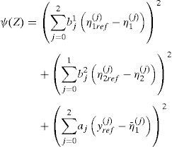
R=100000010000001000000100, P=4.153.2710.616.89, Q=1001 and a0=5.4, a1=2.1, a2=3.4, b01=6,b11=9, b21=1.7, b02=2, b12=8.2. The initial conditions are yp(0)=y˙p(0)=θ˙(0)=0 and θ(0)=−π, the downward position for the pendulum.
The simulation results are presented by Figures 3–5. Figure 3 shows the evolution of the displacement of the cart yp compared to the desired one yref. The simulation results in Figure 3 show that the control scheme provides good tracking. In this figure, there is a perfect agreement between the two trajectories.
.")
.")

Figure 4 shows the evolution of the pendulum angle; indeed, it is a small variation around zero. The evolution of the stabilizing control law is shown in Figure 5. The dynamics of this control signal is quite satisfactory. In fact, there is no unacceptable physical overshoot. One can also see the reduced response time in which the control law stabilizes the controlled variable. This shows very interesting results given by the proposed cascade scheme control.
5.2Ball and beam systemIn this part, a ball and beam is considered. The ball and beam system is an unstable nonlinear system which is well known in automation; therefore, it is regarded as a perfect bench test for the design of control laws for non-minimum phase nonlinear systems.
The ball and beam system is composed of a rigid bar carrying a ball. The latter is characterized by its horizontal axis and its moment of inertia J. Its rotation angle θ compared to the horizontal one is controlled by an engine with direct current to which it applies a couple τ. A ball is placed on the beam where it is able to move with a certain freedom under the effect of gravity, as it is illustrated in Figure 6.

The dynamic model governing the behavior of the ball and beam system in open loop can be expressed by the following equations (Hauser et al., 1992):
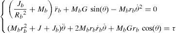
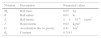
The numerical parameters of the ball and beam system are recapitulated in Table 2. To define a new input u the system can be written in state-space form as (Hauser et al., 1992):
with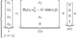
x=rbr˙bθθ˙T, y=h(x) and Bb=Mb/(Jb/Rb2+Mb).
The relative degree of the system is equal to r=3 which is strictly lower than the system dimension n=4.
Applying the procedure of input–output linearization to the system (58) of the ball and beam, the boundary layer system is given by:
its control is given by:with v=y⃛ref+k3ε(y¨ref−y¨)+k2(y˙ref−y˙)+k1(yref−y)and the internal dynamics is given by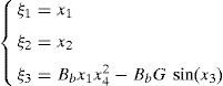

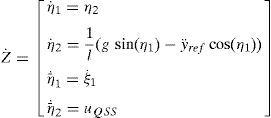
Using Eq. (25), the reduced subsystem can be written as:
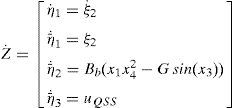
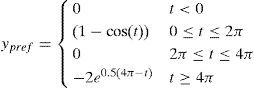
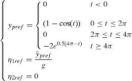
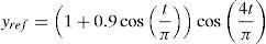
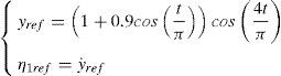
The objective of the studied system control is to ensure that the ball always keeps contact with the beam and that its movement is carried out without slip what imposes a mechanical constraint on the acceleration of the beam. The desired trajectory is characterized by variable amplitude during time and it is given by:
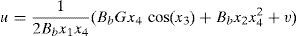
The relative degree of η1 is equal to γη1=2. By using Eq. (26), the descent function will be transformed under the following form:
withthe input u˙QSS=−∂ψ(Z)∂uQSS+1dψ(Z)duQSS−dψ(Z)dxx˙−dψ(Z)dxx˙2+dψ(Z)duQSS2 that stabilizes the internal dynamics is given by solving the problem (25). In simulation, the parameters used for the input–output linearization are: ¿=0.098, k1=4.8, k2=1.7, k3=5.3. For the gradient descent control algorithm, the employed parameters are: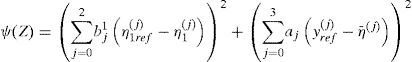
R=70000070000070000070, P=2.3311.438.434.218.665.633.221.344.88, Q=100010001 and b01=3, b11=2.1, b21=1.5, a0=4, a1=7.2, a2=9.1, a3=3.4.
The result of this study is shown by Figures 7–9. Figure 7 illustrates the evolution of the tracking trajectory compared to the desired one yref. In this figure, there is an agreement between the two trajectories. The amplitude variation of the desired trajectory did not hamper the precision of the real trajectory tracking.
 yref (continuous line:

Figure 8 represents the beam deviation angle compared to the horizontal one which is extremely reduced in spite of the consideration of rather severe constraints of displacement.
The control signal represented by Figure 9 is characterized by a very satisfactory dynamics. This explains the important results obtained by the proposed cascade control scheme, characterized by a satisfactory bounded control signal and a better trajectory tracking. This study proves the validity of the control scheme to ensure the high performance control for the ball and beam system.
In fact, the contribution of the cascade control scheme seems to be adapted to the amplitude variation of the desired trajectory.
5.3DiscussionThe main objective of this work was the control of single-input single-output nonlinear systems, using input–output feedback linearization technique.
The proposed methodology is based on input–output feedback linearization, gradient descent control method and singular perturbation theory.
The system is first input–output feedback linearized, separating the input–output system behavior from the internal dynamics. Gradient descent control is then used to stabilize the internal dynamics, using a reference trajectory of the system output. This results in a cascade-control scheme, where the outer loop consists of a gradient descent control of the internal dynamics, and the inner loop is the input–output feedback linearization.
The stability analysis of the cascade control scheme is provided using results of singular perturbation theory. The key idea is to introduce a time-scale separation, enforced by the introduction of a small parameter in the controller. Therefore, the quasi steady state assumption is made, allowing the input–output behavior of the system to be decoupled from its internal dynamics.
Thus, each subsystem is analyzed separately, providing a stability proof of the overall system.
The main contribution of the stability analysis is the global exponential stability of the gradient descent control scheme. The use of singular perturbation theory requires exponential stability results.
Indeed, the application of this methodology to the inverted cart-pendulum and ball and beam systems has shown excellent results.
6ConclusionA cascade control strategy scheme for the tracking problem of non-minimum phase nonlinear systems was presented and successfully applied to the inverted cart-pendulum system and ball and beam model.
This strategy is based on the approximation of the non-minimum phase system by another singular perturbed system. The proposed controller uses the input–output linearization technique to cancel the nonlinearities of the external dynamics and to stabilize the internal dynamics by the gradient descent control algorithm. A stability analysis of the proposed approach has been provided based on the singular perturbation theory. The simulation results have shown excellent results.
Although the approximate input–output feedback linearization was developed in this work for the control of single-input single-output systems, the obtained results can be easily extended to the multi-input multi-output case. On the other hand, the robustness of the proposed approach is not studied in this paper. This could be investigated in the future work.
Conflict of interestThe authors have no conflicts of interest to declare.
Peer Review under the responsibility of Universidad Nacional Autónoma de México.