


In developing and emerging countries progression of informal settlements has been a fast growing phenomenon since the mid-1990s. Half of the world's population is housed in urban settlements. For instance, the growth of informal settlements in South Africa has amplified after the end of apartheid. In order to transform informal settlements to improve the living conditions in these areas, a lot of spatial information is required. There are many traditional methods used to collect these data, such as statistical analysis and fieldwork; but these methods are limited to capture urban processes, particularly informal settlements are very dynamic in nature with respect to time and space. Remote sensing has been proven to provide more efficient techniques to study and monitor spatial patterns of settlements structures with high spatial resolution. Recently, a new feature method, local directional pattern (LDP), based on kirsch masks, has been proposed and widely used in biometrics feature extraction. In this study, we investigate the use of LDP for the classification of informal settlements. Performance of LDP in characterizing informal settlements is then evaluated and compared to the popular gray level co-occurrence matrix (GLCM) using four classifiers (Naive-Bayes, Multilayer perceptron, Support Vector Machines, k-nearest Neighbor). The experimental results show that LDP outperforms GLCM in classifying informal settlements.
In developing countries, informal settlements have become a phenomenon which grow very fast specially in the 21st Century. Half of the world's population is housed in urban settlements. The reason for this phenomenon is the immigration of people from the rural areas to the cities. Many previous studies aimed at extracting houses outline to quantify shape-based features of informal settlements. Object-based image analysis (OBIA) method estimates the size, spacing and shape of the houses by extracting the houses footprint (Blaschke & Lang, 2006). OBIA partitions remote sensing (RS) imagery into meaningful image-objects and assesses their characteristics through spatial, spectral and temporal scale (Hay & Castilla, 2008). Previous studies on geospatial methods have been used to estimate populations and to distinguish the human settlements. For example, a study by Aminipouri, Sliuzas, and Kuffer (2009) estimates the population by creating an accurate inventory of buildings. The computer vision community is facing a very complex and challenging task extracting the spatial data from informal settlements. Constructions in informal settlements are built using various materials and are very close to each other and have no suitable organization. It makes the classification of informal settlements images an uphill task (McLaren, Coleman, & Mayunga, 2005). A number of researchers have tried to develop tools and techniques to characterize the informal settlements areas from remotely sensed data. Mayunga, Coleman, and Zhang (2007) present a new semi-automatic approach to extract buildings from informal settlements images obtained using Quick Bird. Snackes and radial casting algorithm were used to map the informal settlements images. The main limitation in this study is the difficulty of characterizing small houses. Khumalo, Tapamo, and Van Den Bergh (2011) applied two feature methods, Gabor filters and GLCM to distinguish different textural regions in Soweto area (Johannesburg, South Africa). They found Gabor filters more accurate than GLCM in classifying informal settlements. A study carried out by
Ella, Van Den Bergh, Van Wyk, and Van Wyk (2008) compared gray level co-occurrence (GLCM) and local binary pattern (LBP) in their ability to classify urban settlement. It is shown that both methods performed very well with a superior performance for LBP. Van Den Bergh (2011) investigates the powers of two features methods, GLCM and LBP, to classify Soweto (Johannesburg, South Africa) areas. It is established that the performance of the gray level co-occurrence matrix is superior to the local binary pattern on a combined spatial and temporal generalization problem, but the LBP features perform better on spatial-only generalization problems. In Owen and Wong (2013) an analysis is conducted on the shape, texture, terrain geomorphology and road networks to characterize the informal settlements and formal neighborhoods in Latin America. The results achieved were promising when finite data were used to recognize informal settlements. Asmat and Zamzami (2012) introduced an automated house detection technique to extract legal and illegal settlements in Pulau Gaya, Saba. The result shows that the edge to edge features can separate between houses that are less than 2m away from each other. In Graesser et al. (2012), an investigation of nine statistics methods (GLCM PanTex, Histogram of Oriented Gradients, Lacunarity, Line Support Regions, Linear Feature Distribution, Psuedo NDVI, Red-blue NDVI, Scale Invariant Feature Transform, and TEXTONS) is presented with different direction, structure size and shape and tested in four different cities. The GLCM PanTex, LSR, HoG and TEXTON features were found to be the best in characterizing the informal settlements and formal areas. A new feature method, local directional pattern (LDP), based on the known Kirsch kernels was recently proposed by Jabid, Kabir, and Chae (2010a). LDP has mainly been applied in biometrics: face recognition (Jabid, Kabir, & Chae, 2010b), signature verification (Ferrer, Vargas, Travieso, & Alonso, 2010) and facial expression recognition (Jabid, Kabir, & Chae, 2010c). In Shabat and Tapamo (2014) the powers of GLCM and LDP to characterize texture images are compared; the result shows that LDP outperforms GLCM. In this paper, GLCM and LDP are investigated using different numbers of significant bits; the final goal is to identify the most effective amongst them. The computation of the local directional pattern is based on the number of significant bits, and in this work four alternative values are considered: 2, 3, 4, 5 instead of 3 as in the classic LDP.
2Materials and methodsIn the following sections the different feature methods used the in the paper are presented
2.1Gray level co-occurrence matrix (GLCM)In the early 1970s Haralick, Shanmugam, and Dinstein (1973) proposed the extraction of fourteen features, from the GLCM of a gray level, to characterize the image texture. The computation of GLCM depends on two parameters: the orientation θ formed by the line-segment connecting the two considered pixels, and the distance (d)[number of pixels] between them. The direction θ is usually quantized in 4 directions (horizntal – 0°, diagonal - 45°, vertical – 90°, anti-diagonal – 135°).
To compute the gray-level co-occurrence matrix of a window in an image, the following parameters are considered:
- •
The window size, Nx×Ny, where Nx is the number of rows and Ny the number of columns.
- •
Distance (d) and directions θ.
- •
And the range of gray values to consider in calculations 0, …, G−1.
We adopt the formulation used in Bastos, Liatsis, and Conci, 2008 and Eleyan and Demirel (2011) to present the calculation of GLCM. The GLCM is defined as the probability of occurrence of two gray levels at a given offset (with respect to given distance and orientation). Given the image I, of size Nx×Ny, the value of the co-occurrence for the gray values i and j, at the distance (d) and direction θ, Pd,θ(i, j) can be defined as
Where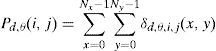
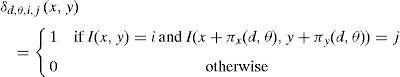
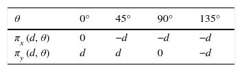
The offset (πx(d, θ), πy(d, θ)) is used to compute the position of (x, y) with respect to its neighbor at the distance (d) and direction θ. For the 4 directions (0°, 45°, 90°, and 135°) and the offsets are given in Table 1.
2.1.1Haralick's featuresGiven an image I with G gray levels, an angle θ and a distance (d), after the gray level co-occurrence matrix, (Pd,θ(i,j))0≤i,j≤G−1, number of features can be extracted, amongst which the most popular are the 14 Haralick features (energy or angular second moment (ENR), contrast (CON), correlation (COV), variance (VAR), inverse different moment (IDM), sum average (SAV), sum variance (SVA), sum entropy (SEN), entropy (ENT), difference variance (DIV), difference entropy (DEN), information measures of correlation (IMC1, IMC2), maximum correlation coefficient (MCC)). The computation of Haralick features is done using a normalized GLCM. The (i, j)th normalized entry,
Pd,θ(i, j), of Pd,θ(i, j) is defined as
where ||Pd,θ||=∑i=0G−1∑j=0G−1Pd,θ(i,j). Details on the calculation of all these features can be found in Haralick et al. (1973). For each texture, T, a chosen distance (d) and a direction θ, 14 Haralick features can be extracted.2.2Local directional pattern (LDP)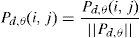
The local binary pattern (LBP) operator depends on the change of the intensity around the pixel to encode the micro-level information of spot, edges and other local features in the image (Jabid et al., 2010a). The gradient is known to be more stable than the gray level; that is why some researches have replaced the intensity value at a pixel position with its gradient magnitude and calculated the LBP (Ferrer et al., 2010). The local directional pattern (LDP) was proposed by Jabid et al. (2010b) to resolve the problem with LBP, mentioned earlier. Since the LBP depends on the neighboring pixels’ intensity which makes it unstable. Instead, LDP considers the edge response value in different direction. LDP features are based on eight bit binary codes assigned to each pixel of an input image. It is composed of three steps (Kabir, Jabid, & Chae, 2010):
- •
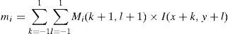
Calculation of eight directional responses of particular pixels using the Kirsch compass edge detector in eight orientations (M7, …, M0) centered on its own position as shown in Figure 1. Given a pixel (x, y) of an image, I, for each direction i, and using the corresponding mask Mi the ith directional response mi can be computed as
For the 8 directions a vector (m7, …, m0) is obtained. Figure 2 shows the Kirsch directional responses of a pixel (x, y). This figure shows a pixel (x,y) that has a gray level 60. (b) Directional responses, together with the ranking of those responses, and the associated bit significance, with m0 being at the less significant position and m7 at most significant position. Note that the ranking of responses is done on absolute values.") Fig. 2.
Fig. 2.Krisch directional response. (a) This figure shows a pixel (x,y) that has a gray level 60. (b) Directional responses, together with the ranking of those responses, and the associated bit significance, with m0 being at the less significant position and m7 at most significant position. Note that the ranking of responses is done on absolute values.
- •
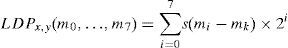
LDP code generation of the directional responses obtained in the previous step. It is based on the selection of k most significant responses and set the corresponding bit to 1 leaving other (8−k) bits to 0. Finally, the LDP code, LDPx,y(m0, …, m7), of the pixel (x, y) with directional response (m0, …, m7), is derived using Eq. (5).
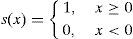
where, mk is the kth most significant response and s(x) is defined asGiven the directional responses generated by the Kirsch convolution on pixel (x, y) presented in Figure 2, the LDP code for k=3 is computed as follows:
- o
m5=270 is the 3rd most significant directional response.
- o
The code of the LDP code of the pixel (x, y) is then
- o
The LDP code, LDPx,y, of the pixel (x, y) is then 49.
- o
- •
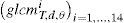
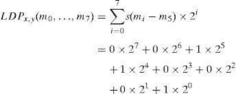
Construction of LDP descriptor which is carried out after the calculation of the LDP code for each pixel (x, y). The input image I of size M×N is then represented by a LDP histogram using Eq. (7), that is also called LDP descriptor. In this case k=3, is used; It means, C38=56 distinct values are generated and used to encode the image. The histogram H obtained from the transformation has 56 bins and can be defined as
where Ci is the ith LDP pattern value, i=1,…,C38 and the definition of p is given in Eq. (9).Given a texture, T, and the number of significant bits k, a feature vector LDPk,T can be extracted and represented as

 This figure shows a pixel (x,y) that has a gray level 60. (b) Directional responses, together with the ranking of those responses, and the associated bit significance, with m0 being at the less significant position and m7 at most significant position. Note that the ranking of responses is done on absolute values.")

Four classifiers are used to evaluate the power of LDP to characterize textures and compared Haralick features extracted from GLCM.
2.3.1Support vector machinesSVM is a learning technique for pattern classification and regression (Cortes & Vapnik, 1995; Vapnik, 2013). It was originally designed as two-class classifier, but many versions have been proposed to perform multi-class classification (Crammer & Singer, 2002; Hsu & Lin, 2002). The principle is, given a labeled set of M training samples (xi, yi), where xi∈R and yi is the associated label (yi∈{−1, 1}), i=1, …, M. A SVM classifier finds the optimal hyperplane that correctly separates the largest fraction of data points while maximizing the distance of either class from the hyperplane. The discriminant hyperplane is defined by the level set function
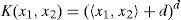
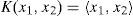
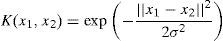
where k(·, ·) a kernel function and the sign of is f(x) indicates the membership of x. Constructing an optimal hyperplane is equivalent to finding all nonzero αi. Kernel function K(xi, xj) is the inner product of the features space K(xi, xj)≤∅(xi), ∅(xj). The three following kernel functions are often used: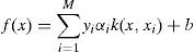
- •
Polynomial kernel
- •
Linear kernel
- •
Radial basic function kernel (RBF)
In our case, the M feature vectors xi=1,…,M are extracted, from texture images that need to be classified, using the local directional pattern, or GLCM.
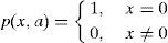
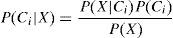
2.3.2Naïve Bayes classifierOne of the most popular and most simplest classification models is the naive Bayes classifier (Friedman, Geiger, & Goldszmidt, 1997). The principle of Naive bayes is: given the training data T which contain a set of samples, each sample X=(x1, …, xn) and there are k classes C1, …, Ck. Each sample is labeled by one of these classes. Naive Bayes predicts a given sample X belongs to the class that has the highest posterior probability conditioned on X. Therefore, sample X is predicted to belong to class Ci if and only if P(Ci|X)>P(Cj|X), for all j such that 0<j<(m−1) and j≠i. By Bayes’ theorem
If the data set has many attributes, it would be expensive to compute P(X|Ci). To solve this problem, naive assumption assumes that the value of the attributes are conditionally independent of one another. This means that
2.3.3k-Nearest neighbor (k-NN)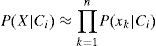
k-NN is a non-parametric classification method introduced in the early 1970s by Fix and Hodges (1951). The process is done by computing the similarity between the sample and the different classes. Let C1, …, Ck be the classes of our samples. Given a new sample X=(x1, …, xn), to find to which class it belongs, the distance d(x, Cj) between x and Cj, for j=1, …, k, is calculated. Sample X is assigned to class Ci0 to which it is closest. Index i0 is calculated as presented in the following equation:
2.3.4Multilayer perceptron (MLP)
MLP is well known and widely used in different detection and estimation applications (Burrascano, Fiori, & Mongiardo, 1999; Gati, Wong, Alquie, & Fouad Hanna, 2000; Kasabov, 1996). The principle of MLP is that the input layer in MLP is considered as layer 0. Assume that the total number of the hidden layers is L. In the hidden layer l the number of node is Nl, l=1, …, L. Let wij be the weight of the connection between the jth nodes of (l−1)th hidden layer and ith nodes of the lth hidden layer, and let xi be the ith input factor to the MLP. Let yil represent the output of the ith node of the lth hidden layer, which can be calculated by the following equation:
where θil represent the bias factor of the ith node of the lth hidden layer, yi0=xi,i=1,…,N0 and f(.) is the active function. Let υki be the weight of the connection between the kth node of the output layer and the ith node of the Lth hidden layer. The MLP output can calculated aswhere the βk is the bias factor of the output layer. The MLP algorithm compares between the network output with the desire output which measures the error in the network. To correct the output layer, this algorithm updates the weight until the output of network gets closer to the desire output.3Experimental results and discussion3.1Data set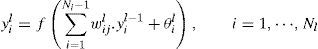
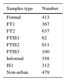
Settlements image categories, shown in Figures 3–8, were identified in Soweto (Gauteng province, South Africa) to work with as target classes. Data used are gray-level images with 8 bit per pixel, and a size of (200×200) pixels. Table 2 shows the number of samples in each category.
- •
Formal township (FT1, FT2): The structure of the formal township building is placed in a planned manner. The difference between FT1 and FT2 relates to the size of the houses.
- •
Informal squatters (IS): The structure of the informal squatters is not stable. The dwellings of this category are shack type (made out of cardboard, wood, tin, etc.). This is typically characterized by high building density.
- •
Formal township+informal squatter (FTIS1, FTIS2, and FTIS3): In this category we can establish any type of any density, of residential unit, but buildings appear in pairs and a larger building is accompanied by a backyard shack.
- •
Informal township: The structure of the informal township is recognized as a constant or semi-constant structure. The dwelling of this category is shack type and located on serviced and un-serviced sites. The dwelling density varies from low to high.
- •
Formal: The structure of the formal residential is a constant structure, located near well establish buildings area.
- •
Non-urban area: The areas outside a town or a city. Open swath of land that has few homes or other buildings.

: the structure of the informal squatters is not stable. The dwellings of this category are shack type (made out of cardboard, wood, tin, etc.). Typically characterized by high building densities.")
: In this category we can find any type of any density, of residential unit, but buildings appear in pairs a larger building will be accompanied by a backyard shack.")


The computation of GLCM is done using the following parameters:
- •
Number of gray levels: 256
- •
Directions: 0°, 45°, 90°, 135°
- •
Distance: 1
The computation of the local directional pattern is based on the number of significant bits, and in this work four alternative values are considered: 2, 3, 4, 5.
3.2Result and discussionPerformance of the various classifiers using various size of training samples, with various values for k are considered. k-NN and MLP achieve reasonably good results, even when only a small proportion of the data is used for training. The superiority of the k-NN and MLP over both SVM and NB is easily perceptible. Moreover, it can be noticed that when the number of significant bits (k) changes from 2 to 4 the accuracy improves and declines when k=5. Classifiers have the best performance for k equal 4 and the worst performance is registered for k equal to 2. The performance of LDP is evaluated for different values of k: The average accuracy of LDP with different k values shows that for LDP when k equal 4 is the highest performance (85.6%) compared to the rest. For LDP, the value 2 for k is the lowest performance (77.7%). The best achievement was obtained by k-NN and MLP 98.9%, 98.19% in LDP (4) and LDP (3) when the data proportion is 80% as training 20% testing. NB performances are remarkably low ranging between 55% and 70%. Another observation is the fact that the accuracy of SVM is not very high either. With the gray-level co-occurrence matrix, different combinations of the 14 original Haralick features (entropy, (entropy+IDM), (energy+contrast+correlation), (entropy+energy+contrast), (energy+correlation+entropy+IDM), (entropy+energy+contrast+correlation+IDM), and all 14 features are used to characterize textures. The presentation of different feature combinations to characterize informal settlements reveals that the best performance is achieved by k-NN with value (86.04%) using the 14 original Haralick features in 45° direction. With NB, the performance is remarkably low ranging between 29% and 53%. Another observation is that both SVM and MLP are not very effective classifying informal settlements, with accuracies ranging from 30% to77%. Using k-NN, the best achievement was achieved with 45° direction at 91%. With NB, the performances are remarkably low ranging between 50% and 55% The accuracy of both SVM and MLP are not very high range between (48%–60%) and (64%–80%). The best performance was achieved in 45° direction with value (80%) using MLP and (60.81%) using SVM. The training set percentage: the average accuracy of the best direction changes from 62% when the training set is 10%–71.17% when the training set is 80%. With the knowledge that the best performance is achieved with GLCM and this when the 14 original Haralick features at 45° direction are chosen, it can be compared to the performance of LDP when k equals 4. The average performances of each classifier in both feature methods are such that, with NB and SVM, the performance is remarkably low in both LDP (4) and GLCM (45°), the best achievement is (83.06%) by SVM using LDP (4). With MLP, LDP (4) achieved 20% more with value (92.77%) compared to GLCM (45°) with value (77.48%). With k-NN, The best result was achieved by LDP (4) with value (92.7%), compared to GLCM (45°) with value (86.03%). For GLCM (45), we find the performance from 20% to 80% increase by approximately 1% in each step. The best achievement obtained when the training set is 80% with a value (71.17%). The worst achievement obtained when the training set is 10% with a value (62.6%). For LDP (4), we find the performance almost constant from 50% to 80% with value (86.81%). The best achievement obtained when the training set is 80% with a value (86.81%). Figures 9–10 below summarize the comparison between these two methods (LDP, GLCM). In conclusion, the best combination used in our approach is using the local directional pattern with k equals four applying on nine categories of image, and the k-nearest neighbor being the preferred classifier.

.")
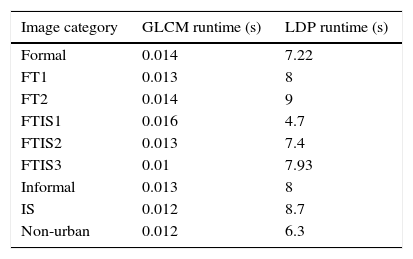
For an image of size n×m, GLCM running time will be G(m, n)=O(mn). However, the running time for LDP is L(m, n)=R(m, n)+H(m, n) where R(m, n)=O(mn) is the running time to compute the responses and H(m, n)=O(mn) is the running time of the computation of the histogram, then L(m, n)=O(mn). Table 3 shows running times for both GLCM and LDP applied to nine different categories using a computer with a processor Intel Core i5, a CPU of 2.3GHz and 4G of RAM. With GLCM 14 features were computed and for k equals 4 for LDP; the running time of the GLCM algorithm is remarkably low (less than 13ms to process an image). Compared to LDP, which takes a very long time to compute, ranging from 4.7s in average to process an image in FTIS1 to 9s in FT2. It is worth mentioning that the size of each image is (200×200).
5ConclusionTwo feature methods, local directional pattern (LDP) and gray-level co-occurrence matrix (GLCM), have been compared using four different classifiers (Naive-Bayes, multilayer perceptron, support vector machines, and k-nearest neighbor). This work has investigated the impact of the number of significant bits considered to code the Kirsch masks application responses. Experiments have shown that the choice of 4 significant bits achieves the best accuracy for texture characterization using LDP. It has also been established that the best texture feature is the local directional pattern when k-NN is used as a classifier. On the other hand, it has been demonstrated that the local directional pattern is superior in characterizing informal settlement images. However, the running time for LDP is two orders of magnitude higher than that of the GLCM.
Conflict of interestThe authors have no conflicts of interest to declare.
Peer Review under the responsibility of Universidad Nacional Autónoma de México.