A Bayesian Combination Forecasting Model for Retail Supply Chain Coordination

Abstract

Retailing plays an important part in modern economic development, and supply chain coordination is the research focus in retail operations management. This paper reviews the collaborative forecasting process within the framework of the collaborative planning, forecasting and replenishment of retail supply chain. A Bayesian combination forecasting model is proposed to integrate multiple forecasting resources and coordinate forecasting processes among partners in the retail supply chain. Based on simulation results for retail sales, the effectiveness of this combination forecasting model is demonstrated for coordinating the collaborative forecasting processes, resulting in an improvement of demand forecasting accuracy in the retail supply chain.

1

Introduction

The supply chain coordination among partners throughout the entire supply chain has abstracted more and more attention from both the industries and the academics [1]. Various supply chain coordination solutions have been developed to streamline the supply chain management and improve the supply chain operations performance [2-4]. Collaborative planning, forecasting and replenishment (CPFR), which is an retail supply chain coordination innovation, has been adopted and implemented by many world-renowned retailers and manufacturers, such as Wal-Mart and Proctor & Gamble. CPFR concerns the collaboration where two or more parties in the supply chain jointly plan a number of promotional activities and work out synchronized forecasts, on the basis of which the production and replenishment processes are determined. The first CPFR project was piloted by Wal-Mart with its suppliers in 1995. The results of the two-year project showed that CPFR could simultaneously reduce inventory levels and increase sales for both retailers and suppliers. Since its original application was initiated, CPFR has had many successful applications in North America, Europe and China [5,6].

The collaborative forecasting plays an important part in the CPFR implementation procedure. In this paper, we will briefly review the CPFR concept and its implementation process at first. The collaborative forecasting process which is the core part of CPFR will then be mainly discussed. The collaborative forecasting process is the basics phase of the implementation of CPFR and the cornerstone to the success of CPFR projects. The collaborative forecasting process of CPFR requires a solid forecasting approach to synthesize information and knowledge from multiply parties in the supply chain. The combination forecasting method can combine forecasting models from different parties to smooth the coordination in the supply chain and reduce forecasting discrepancies. Thus, considering the multiple forms of forecasting resources in the retail supply chain, the Bayesian combination forecasting method is applied for CPFR collaborative forecasting modeling with improved forecasting accuracy and supply chain collaboration performance in this paper.

Combining forecasts is a well-established procedure for improving forecasting accuracy which takes advantage of the availability of both multiple information and computing resources for data intensive forecasting [7]. Since Bates-Granger first proposed the combination forecasting method in 1969 [8], many kinds of combination methods have been developed [9]. Bayesian combination methods [10, 11] use the distributional properties of the individual forecasts to construct the combination. Many researches related to Bayesian combination methods have been developed in many schemes. Walz and Walz [12] compared the Bayesian methodology and multiple regression composite forecasts with macroeconomic data. And their study found that the Bayesian combination procedure produces more accurate composite forecasts than does the regression combination procedure. Hoogerheide et al [13] compared several Bayesian combination schemes in terms of forecast accuracy and economic gains. Faria and Mubwandarikwa [14] studied a nonlinear geometric combination of Bayesian forecasting models. The Bayesian combination forecasting can combine the quantitative and qualitative data and forecasting methods [15]. Demand forecasting in retail supply chain is impacted by many factors such as product promotion or social development trend. Also, subjective forecasting based on the expert experiments is often used in retail market forecasting. The Bayesian combination forecasting model is therefore considered to be a suitable collaborative forecasting approach in retail supply chain coordination.

In the first part of this paper, the CPFR retail supply chain coordination and collaborative forecasting process are discussed briefly. In the second part of the paper, a Bayesian combination forecasting method is modeled to coordinate forecasting process in retail supply chain. Finally, the simulation of this model is completed using Carrefour sales data. The simulation results showed the effectiveness of this Bayesian combination forecasting model in retail supply chain collaboration process

2

CPFR collaboration and forecasting

CPFR, which was proposed by VICS (Voluntary Inter-industry Commerce Standards Association) in 1995, provides retailers and suppliers with a framework for sharing key supply chain information and coordination plans. Under CPFR, supply chain partners form a consensus forecast, either by working collaboratively or by first developing their own individual forecasts, which are then used to create a consensus forecast. The key to collaboration utilizing CPFR is the jointed demand forecast between retailers and manufacturers, which is then used to synchronize replenishment and production plans throughout the entire supply chain. This coordination and information sharing allows retailers and suppliers to optimize their supply chain activities. Dirk Seifert, a professor at Harvard Business School and the University of Massachusetts, defined CPFR as “an initiative among all participants in the supply chain, intended to improve the relationships among them through jointly managed planning processes and shared information.”[16].

The collaborative forecasting process, which is one of main CPFR phases that includes collaborated plan, forecasting and replenishment phases, guarantees a precise demand by implementing a jointed forecasting process inside the retail corporation and among its supply chain partners. The forecasting accuracy, an index used to evaluate the performance of CPFR collaborative forecasting process, is determined by the forecasting discrepancies between the forecasting results and actual demand values. The forecasting discrepancies may be caused by inaccuracy of the input data or differences among forecasting models used by different partners. Inaccuracy of input data may be resulted from inaccurate and untimely sale data and the un-timely communication for changes caused by demands, such as alteration of advertisement plan or products promotion plan. A CPFR collaborative forecasting process among partners can help to improve the accuracy of data for forecasting. In this paper, we will focus on the discussion of the ways to reduce discrepancies caused by forecasting models differences. The Bayesian combination forecasting model is proposed to reduce this kind of discrepancy and improve the demand forecasting accuracy and collaboration in the CPFR implementation process.

In the CPFR collaborative forecasting process, partners in the supply chain will use different forecasting models and forecasting cycles because of their different forecasting knowledge backgrounds and resources. For example, in order to forecast products demand the retailers may use the simple moving average method, while the manufacturers may use artificial neural network method. Also, the retailer’s forecasting cycles could arrange from several weeks to one quarter, due to large differences among various kinds of sale items. However, the manufacturers may take one week as their forecasting cycle due to fewer kinds of products. This may results in more accurate forecast results by manufacturers because of shorter forecasting cycle and more sophisticated forecasting models. Demand forecast results may differ by as much as a factor of three between manufactures and retailer fro the same product [17]. In order to reduce these forecasting discrepancies and smooth the collaborative forecasting process among CPFR partners, a jointed forecasting model which can combine forecasting models from different parties should be used. The combination of the complex forecasting models and professional forecasting knowledge used by manufacturers and timely sales data and market information sourced from retailer will improve the forecasting accuracy and effective supply chain collaboration.

The combination forecasting method which tries to combine the different forecasting approaches used by retailers and manufacturers is necessary for more accurate and effective collaborative forecasting in CPFR process.A simple approach might be easy for forecasting, but the slightly more complex combination forecasting method can improve forecasting accuracy in the CPFR collaborative forecasting process.

The combination forecasting approach that we developed can reduce the forecasting discrepancies resulting from the different interests of retailers and manufactures in the supply chain. In general, retailers might concern more with sales loss caused by goods shortage, while manufacturers may concern more about overstock cost resulting from surplus stock and transportation cost caused by returned goods. A jointed forecasting model can combine both parties’ considerations in the retail supply chain.

The CPFR collaborative forecasting process based on the combination model is showed as the flowchart in Fig.1. Based on the data from point-of-sale, initial forecasting results are calculated by combination forecasting model that combines individual forecasting models from the retailer and the manufacturer.

Figure 1.

CPFR Combination Forecasting Process Flowchart.

And then, the final optimized forecasting report is created after correcting discrepancies in the forecasting result that cannot be accepted according to the CPFR exception standard.

The exception standard is jointly created by retailers and manufacturers. The collaborative forecasting process among the parties in the supply chain can help to reduce forecasting discrepancy caused by inaccuracy of input data. The combination forecasting method applied in CPFR collaborative forecasting process can reduce forecasting discrepancy resulting from forecasting models differences between retailers and manufacturers.

3

Bayesian combination forecasting modeling

Individual forecasting methods available to the forecaster range from applying the robust simple average to the far more theoretically complex, such as methods based on artificial neural networks methods [18]. Various optimal estimation theories, such as the least squares, the weighted least square, minimum variance, and minimum variance unbiased estimation procedures have been applied to find out proper techniques to combine individual forecasts. Among various kinds of combination formulations, the simple average combination forecasting method has the virtues of impartiality and robustness in economic and business forecasting [19]. All the methods adopt the linear formulation whereby a vector, f, of n individual forecasts are combined via a linear weighting vector, w. In the simple average method the weight of n individual forecasts are the same as w=1n.

The combination method proposed by Bates and Branger in 1969 is referred to as the optimal linear combination model or B-G method. With this approach, the forecasting results f_c1, f_c2…f_cn are assumed to be random variables with the covariance matrix ∑. Based on the minimizing the variance criteria (MV), the optimal forecasting results can be calculated as the following Eq. 1.

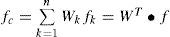
Here, the weighting vectorWT=1nTΣ−11n−11nTΣ−1=W1,W2...,Wn1nT=1,1,...1

The Bayesian combination forecasting model can be developed from the B-G method, using the distributional properties of the individual forecasts to construct the combination. Suppose Y is a vector representing sampled actual demand. The forecasting results obtained from the different parties in the supply chain which are forecasted with m individual forecasting methods are represented by f₁,f₂…f_m, j = 1,2,m. And, i = 1,2,n present different forecasting time periods. The Bayesian combination forecasting method makes use of the Bayesian rule to decide the optimal combination ways and weights of individual forecasting methods in combination model, resulting in combined forecasting results in different time periods fˆ_ic(i=1,2, …, n), which can approximate actual demand values.

Set ZiT=f1, f2, …, fm, i = 1,2,…,n. Then the joint probability density function of m individual forecasting samples on independent time z₁, z₂,…,z_n can be calculated as the following Eq. 2.

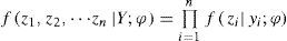
Here ϕ is a parameter vector, and Y^T = (y₁,y₂,…,y_n) is the vector of the actual demand samples on the different forecasting time periods.

According to the Bayesian rule, the probability density function that Y is set as a specific vector value y can be calculated as the following Eq. 3:

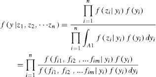
Here, f(y_i)(i = 1,2,…, n) is the prior probability distribution of y_i, which represents the prior estimation or preference of decision maker to y_i. A_i is the definition set of y_i.

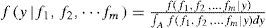
If only one forecasting time period is considered as the general case and prior distribution f (y) is uniform distribution form, that is f (y) ∝ 1, the Eq. 2 can be simplified as the following Eq. 4.

The forecasting error distribution of individual forecasting results (f₁,f₂,… f_m) is chosen as normal distribution or logarithm normal distribution in most cases. In this paper, a more general distribution of forecasting error is introduced through Box - Cox conversion, where

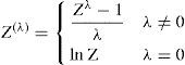
Here, λ is conversion parameter

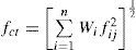
Supposed ∑ is the covariance matrix of (f₁, f₂,…f_m) and W_i represents the weights of individual forecasting methods f_i. Then, the weights can be calculated as following Eq.6, based on the minimum error variance criteria:

And, nonlinear combination forecasting formula can be obtained through Bayesian analysis as following Eq.7, which will be used to calculate the optimal combination forecasting results approximating to the actual values in vector Y.

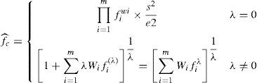
Here,1S2=1mTΣ−11m=1Σ1mTΣ*1m, and ∑i=1nWit=1.

And, the optimal conversion parameter λ^* can be calculated as the following Eq.8.

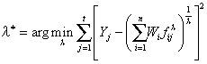
Where f_ij is the forecasting result on j time period through i individual forecasting method. The weights W_i can be calculated by Eq. 6. The covariance matrix ∑ can be determined from prior value or estimated by past approximate sample values.

4

Simulation

Carrefour is one of the biggest supermarket chains in the world. Carrefour shares the sales data with its suppliers through the Internet technology and coordinates the forecasting process with the partners in the retail supply chain.

To demonstrate our proposed model, simulation of the Bayesian combination forecasting approach will be based on the sales data of one kind of biscuit products in Carrefour China.

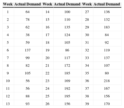
Detailed sales data of this product for 39 weeks is showed in table 1. During the simulation process, the sales data from week 1 to 28 were used to estimate parameters for the Bayesian combination forecasting model. The sales data from week 29 to 39 were used as a comparison with the forecasting results obtained from combination forecasting methods.

Table 1.

The Sales Data for Carrefour Biscuit Product.

Week	Actual Demand	Week	Actual Demand	Week	Actual Demand
1	64	14	100	27	136
2	78	15	110	28	132
3	62	16	135	29	183
4	38	17	124	30	84
5	59	18	105	31	92
6	137	19	86	32	119
7	99	20	117	33	137
8	82	21	172	34	107
9	105	22	185	35	80
10	56	23	169	36	218
11	56	24	192	37	167
12	88	25	195	38	156
13	93	26	156	39	170

The distribution curve of biscuit product sales data over the entire 39 weeks is showed in Figure 2. Through a statistical analysis of the biscuit sales data, including sample autocorrelation function (ACF) testing and partial correlation testing, it was found that distribution of the biscuit sales values y_i is a first order stationary sequence I(1).

Figure 2.

Product Sales Data Distribution Curve in 39 Weeks.

4.1

Individual forecasting method selection and Bayesian combination determination

Based on the Carrefour biscuit sale data and statistical analysis, the Bayesian forecasting model can be created following three main steps, which includes proper individual forecasting method selection, combination determination and optimal parameter estimation.

The characteristics of individual forecasts combining in the model has substantial implications on the overall forecasting performance of model, and thus it is very important to rigorously analyze individual forecast errors. The first step in the combination modeling process is to compare and select suitable individual forecasting methods for combination.

In general, different parties in the retail supply chain may use different patterns of forecasting. So, the different patterns of individual forecasting methods, which include simple moving average, exponential smoothing, trend extrapolation, ARIMA (autoregressive integrated moving average) and artificial neural network methods, are applied to create a combined model to forecast product demand from week 29 to 39.

Through a comparison study of forecasting results from each individual forecasting method, the best parameters of each individual forecasting method are estimated.

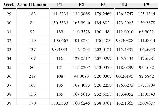
The forecasting results of five individual forecasting methods are indicated in Table 2. The F1 column indicates the best results forecasted by the simple moving average method using a moving period N =3. The F2 column is the best results forecasted by the exponential smoothing method with the smoothing coefficient a = 0.6. The F3 column is the best results forecasted by the two polynomial regression method (n=2). The F4 column is the best results forecasted by the ARIMA method when parameter d = 1. The F5 column indicates the best results forecasted by the artificial neural network method with three neurons and two hidden layers in the neural network.

Table 2.

Forecasting Results of Five Individual Forecasting Methods.

Week	Actual Demand	F1	F2	F3	F4	F5
29	183	141.3333	138.9865	179.2469	136.3747	125.3344
30	84	150.3333	165.3946	184.8024	173.2965	159.2878
31	92	133	116.5578	190.4484	112.6916	68.3652
32	119	119.6667	101.8231	196.185	93.30308	111.0044
33	137	98.3333	112.1293	202.0121	115.4397	106.5959
34	107	116	127.0517	207.9297	135.7434	117.6981
35	80	121	115.0207	213.9379	118.0299	93.1682
36	218	108	94.0083	220.0367	90.26195	82.5842
37	167	135	168.4033	226.2259	186.0273	177.1399
38	156	155	167.5613	232.5058	183.4052	115.0543
39	170	180.3333	160.6245	238.8761	162.1665	150.9677

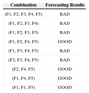
After the five individual forecasting methods are selected, the second step in combination modeling process is to determine suitable ways to combine these individual methods. With the Matlab simulation tool, the forecasting results are calculated using different ways of combining these individual forecasting methods, as shown in Table 3. As it is widely accepted that only ‘‘good’’ forecasts should be included in a combination, serious differences in forecast error variances between the individual forecasts are not to be expected [18]. From the forecasting results shown in Table 3, it can be seen that any combination ways that included F3 polynomial regression method did not have good forecasting performance. So, F3 individual forecasting method was dropped.

Table 3.

Different Combination of Individual Forecasting Methods.

Combination	Forecasting Results
(F1, F2, F3, F4, F5)	BAD
(F1, F2, F3, F4)	BAD
(F1, F2, F3, F5)	BAD
(F1, F2, F4, F5)	GOOD
(F1, F3, F4, F5)	BAD
(F2, F3, F4, F5)	BAD
(F2, F4, F5)	GOOD
(F1, F4, F5)	GOOD
(F1, F1, F5)	GOOD

Finally, the four individual methods (F、F2、F4、F5) were chosen for the Bayesian combination model.

4.2

Bayesian combination model simulation

As the conversion parameter λ in the Bayesian combination Eq. 7 varies, Bayesian combination formula can be simplified into the different forms of other simple combination forecasting methods. For example, when λ =2, Bayesian combination form can be approximated into the following Eq. 9, which has the same combination form as the weighted average of square sum.

When, λ = 1/2, Bayesian combination forms is as the following Eq. 10, which has the same combination form as the weighted average of square root.

And, when λ=-1, Bayesian combination forms is as following Eq. 11, which has the same combination form as the weighted average of harmonica series.

The optimal conversion parameter λ^* is calculated according to the Eq. 8. The fitting process of the optimal parameter λ^* is shown in Figure 3. From the fitting curve, it can be seen that the sum of square of forecasting error is minimized when λ^* = 6.9419, which could be rounded to λ^* =7 for the Bayesian combination modeling.

Figure 3.

Bayesian Parameter λ Fitting Curve.

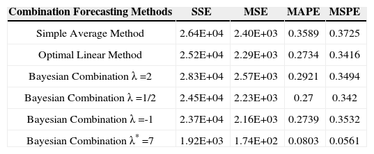
Errors between forecasting result and actual demand, representing forecasting discrepancy, are used as the evaluation standards of forecasting methods performance. Here (see Table 4), we have used four main measure indices of forecasting error, which are the sum of squares error (SSE), the mean square error (MSE), the mean absolute percentage error (MAPE) and the mean square percentage error (MSPE), to evaluate the accuracy of forecasting results from Bayesian combination forecasting model.

Table 4.

The Comparison of Bayesian Combination Models Forecasting Errors.

Combination Forecasting Methods	SSE	MSE	MAPE	MSPE
Simple Average Method	2.64E+04	2.40E+03	0.3589	0.3725
Optimal Linear Method	2.52E+04	2.29E+03	0.2734	0.3416
Bayesian Combination λ =2	2.83E+04	2.57E+03	0.2921	0.3494
Bayesian Combination λ =1/2	2.45E+04	2.23E+03	0.27	0.342
Bayesian Combination λ =-1	2.37E+04	2.16E+03	0.2739	0.3532
Bayesian Combination λ^* =7	1.92E+03	1.74E+02	0.0803	0.0561

The Bayesian combination models with different parameter λ are compared with the simple average method and optimal linear method in the simulation based on Carrefour biscuit sales data. The forecasting errors of different combination forecasting methods are shown in the table 4. The measure of forecasting error with the optimal Bayesian combination method when λ^* =7 are lower than those of simple combination methods and other Bayesian combination methods when λ =-1, λ =1/2, and λ =2, indicating that these choices of λ are the most suitable for combination models in the retail collaborative forecasting process. This research shows that the Bayesian combination forecasting method is an effective approach for integrating and coordinating the forecasting process among partners in the retail supply chain. And, the optimal Bayesian combination forecasting method can highly improve the demand forecasting accuracy of collaborative forecasting activity in the retail supply chain.

5

Conclusion

The collaborative planning, forecasting and replenishment framework provides a practical roadmap for retail supply chain coordination. This paper proposed a Bayesian combination forecasting model that can combine individual forecasting methods from different parties in the retail supply chain for CPFR collaborative forecasting. Simulation results using a real example indicate that forecasting discrepancies are reduced and collaborative forecasting accuracy is improved when the forecasting process are integrated through the optimal Bayesian combination forecasting model. This suggested that the Bayesian combination forecasting method is an effective approach for the collaborative forecasting process in retail supply chain. Further research on collaborative forecasting methodologies for supply chain coordination will be extended into more complex product demand situations in the future.

Acknowledgements

This research was partly supported by grants from the Shanghai Science Foundation Council (12ZR1400900), the Chinese National Science Foundation Council (71172174), Foundation of Ministry of Education of China (20110075110003), Innovation Program of Shanghai Municipal Education Commission (12ZS58) and National Key Technology R&D Program of the Ministry of Science and Technology (2012BAH19F00). Thanks to the editor and referees at the Journal of Applied Research and Technology.