Two algorithms to compute the electric resistivity response using Green's functions for 3D structures

Resumen

Se introduce una solución integral para el problema directo de la respuesta geoeléctrica DC para cuerpos tri-dimensionales en un semi- espacio, mediante las funciones de Green. El primer algoritmo que se presenta se basa en el método integral de volumen (MIV); aquí, únicamente la corriente eléctrica primaria se utiliza para calcular el potencial eléctrico. El segundo caso emplea el método integral de superficie (MIS), en donde se asume que la carga inducida es debida al campo eléctrico primario. Ambos algoritmos son una combinación de integrales de volumen y de condiciones de frontera. Este artículo muestra la aplicabilidad de estos algoritmos para generar imágenes de perfiles de resistividad que reproducen algunos arreglos de electrodos para ejemplos sintéticos tradicionales, y posteriormente estas imágenes se comparan con resultados ya publicados en la literatura. Finalmente, la comparación entre estos resultados muestra que el concepto de carga inducida utilizada en MIS produce una mejor aproximación, que el esquema MIV en el cálculo del potencial eléctrico.

Abstract

An integral solution of the forward DC geoelectric response for three-dimensional target-bodies in a half-space, based on Green's functions, is introduced. The first algorithm presented is based on a volume integral method (VIM); here, only the primary electrical current is involved to compute the electric potential. The second one employs the surface integral method (SIM), and it is assumed the induced charge is due to the primary electrical field. Both algorithms are a combination of boundary and volume integrals. This paper shows the applicability of these algorithms to generate resistivity profile images reproducing some electrode arrays for traditional synthetic examples, and then these images were compared with already published results. Finally, the comparison between results shows the concept of induced charge used in SIM produces a better approach than VIM scheme in computing the electrical potential.

Introduction

The last three decades have been characterized by an increased use of computerized methods in the interpretation of geoelectrical data, due to the evolution of the computer systems. Most reconstructive algorithms are iterative and need a forward solution, i.e., to compute the electrical response for a given resistivity distribution and a given set array of current injection electrodes. Thus, the electrical potential needs to be calculated at a set of measured points. This forward problem consists on solving an elliptic partial differential equation (PDE): the Poisson equation, with boundary conditions. The formulation leads to solve a system with two kinds of unknown quantities: the electrical potential and a current-related quantity.

The PDE problem is usually solved with finite-difference schemes that specially has been helpful to compute the apparent electrical resistivity in a two-dimensional medium (e.g. Forsythe and Wasow, 1960; Mufti, 1976; Dey and Morrison, 1979; Marchuk, 1989; Thomée, 1989; Spitzer, 1995; Zhang et al., 1995; Loke and Barker, 1996). Another scheme extensively used in solving this PDE problem has been finite-element scheme (e.g. Coggon, 1971; Strang and Fix, 1973; Wait, 1977; Fox et al., 1980; Pridmore et al., 1980; Johnson, 1987; Ciarlet, 1991; Sasaki, 1994; Tsourlous and Ogilvy; 1999; Li and Spitzer, 2002, 2005; Marescot et al., 2008; Ren and Tang, 2010). Finite volume schemes have also produced excellent results in computing electrical resistivity (e.g. Snyder, 1976; Baliga and Patankar, 1980; Cai et al., 1991; Eskola, 1992; Perez-Flores, 1995; Perez-Flores et al., 2001; León-Sánchez, 2004; Pidlisecky et al., 2007). The methods based on a finite-element scheme have been widely studied in the past 40 years and give rise to very high-performing techniques as mixed methods (Lesur et al., 1999), or h-p methods (Babuska and Suri, 1994). Nevertheless, the already mentioned methods lead to very large systems of linear equations, which are very demanding even for the supercomputers.

One limitation in integral methods is the heterogeneity of the medium and the geometrical complexity of the bodies immersed in the modeled medium. An alternative to reduce this limitation is to propose a linearization procedure or some hypothesis about the interaction between bodies, as the weak scattering problem (Eskola, 1992; Hvozdara and Kaikkonen, 1998). Such alternatives make integral equation method a good option to solve PDE, since this method does not need linearization, even in the case of bodies with complex geometry.

The boundary-element methods (BEM) (Okabe, 1981; Nedelec, 1985, 1994; Wendland, 1987) can be thought as a particular version among the finite-element methods. An example of the application of this method to 3-D electrical modeling can be found in Poirmeur and Vasseur (1988). In this methodology, only the boundaries between media, of constant resistivity, need to be discretized and integrated. Therefore, unbounded homogeneous media are easily treated, and 3-D problems are solved using only 2-D integrals. Moreover, the boundary- element method can be coupled with standard finite element methods. The modification of the integral equations method with BEM, introduced by Hvozdara and Kaikkonen (1998), is physically more meaningful and not so much demanding on computer resources, which made the method more accessible for routine prospecting work.

This work follows the integral solution of the forward DC geoelectrical problem introduced by Hvozdara and Kaikkonen (1998; Hvozdara, 1982), which consists of interpreting the electric response of three-dimensional disturbing body of non-uniform conductivity, immersed in a planar homogeneous half-space, under the assumption of weak scattering (Figure 1). In this research two algorithms are proposed to solve this forward problem, by introducing the resistivity contrast between bodies and the homogeneous half-space and the concepts of:additive potential sources for immersed bodies and density surface charges, which result in two types of solutions: volume (VIM) and surface integral methods (SIM). SIM and BEM use the same theoretical background but the boundary surfaces in SIM are not discretized and therefore no finite element is employed. SIM and VIM are used to solve the geoelectrical problem, with mixed boundary conditions, by considering a dipole-dipole electrode array to reproduce an electric tomography profile. The results of some synthetic examples are compared with those obtained by alternative methods in solving PDE already published by other authors (e.g. Tsourlos and Ogilvy, 1999; Pridmore, 1978; Hvozdara and Kaikkonen, 1998; Perez-Flores et al., 2001).

Figure 1.

Conceptual model of a heterogeneous half-space formed by some bodies, with different but constant resistivity values, ρ₁ ...ρ₆, immersed in a homogeneous medium with a constant resistivity value ρ₀.

Theoretical Setting

For a 3D heterogeneous half-space with a resistivity ρ (r¯), the total electric potential for a point source at the surface z = 0, is expressed by:

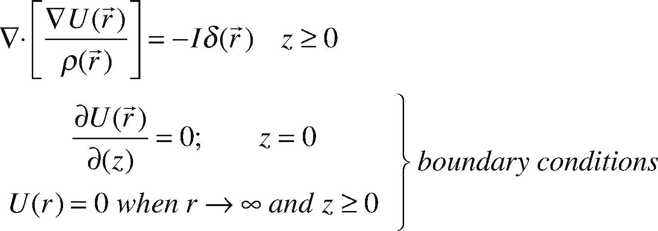
This PDE problem with boundary conditions can be rewritten as:

One solution for this equation can be expressed for the potential U(r) using the Green's theorems and Green's function method:

where r→ ′=(x ′, y ′, z ′) is related to local coordinates system, r→⁼(x, y, z) related to global coordinates system, and ∮s  denotes the integral over the boundaries s. In particular the integral over all boundaries can be written as: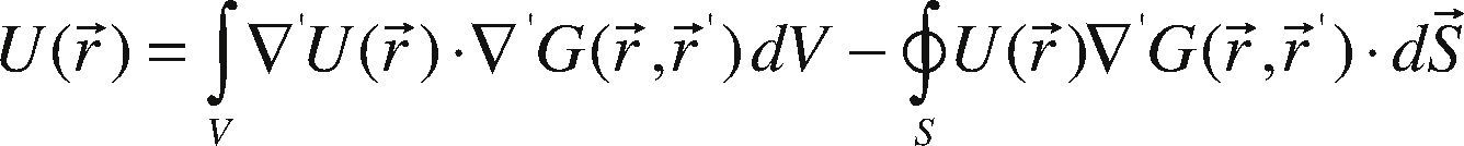

Where ∮s U (r→)▿′ G(r→,r→) dS→0 if, r→→∞ due to the boundary conditions (Hvozdara and Kaikkonen, 1998), and G is the Green's function. Green's function, G, is is defined for a half-space problem (eq. 3) for Neumann condition, where ∂G∂Z z=0=0.

∇′U(r→ ′) −E→(r→ ′) and by using E→(r→′) ρ(r→′)J→ (r→′), the expression (3) can be rewritten as

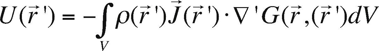
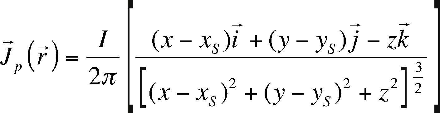
The Volume Integral Method (VIM) evaluates U(r) from equation (4), so it is necessary to know the current density function J→(r→) in half-space. The computation of J→(r→) is not an easy task, since there are several types of currents involved, particularly those present in the heterogeneous half-space. The “weak scattering problem” assumes that the primary conduction current is more significant that the secondary, that is J→ 2r→<Eskola, 1992). Due to the interaction between bodies, we can express J→ p(r→) as:

where sub-index s represents the location of source electrodes.

The Neumann Green function for half space can be defined, as was done by Kaufman (1992) as:

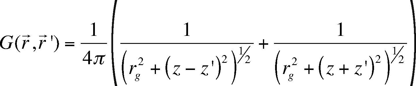
where rrg2= (x − x′)2 + (y − y′)2. Introducing this definition into eq. 4, and evaluating eq. 5 in z= 0, it becomes:

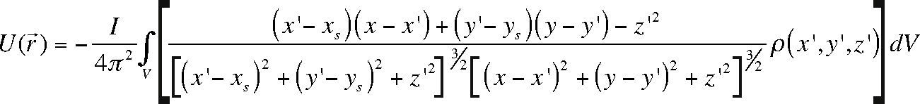
Gómez-Treviño (1987), Pérez-Flores et al. (2001) and León-Sánchez (2004) used a similar relation to estimate the apparent resistivity ρ(r→) in a heterogeneous half-space.

Also U(r→) can be expressed as a surface integral, leading to the Surface Integral Method (SIM).If ρ (r→) J→ (r→) E→ p(r→)=E→ p(r→)+E→ 2(r→) then eq. (4) can be rewritten as

Here E→_p (r→) is the primary electrical field due to the point source and E→₂ (r→) the secondary electric field due to the heterogeneities of the medium.

The first term of the right hand of equation (7) is equal to the primary source's potential U_p (r→). The second term implies the whole halfspace volume. This integral could be separated in volumes for each heterogeneous body, for instance if we define:

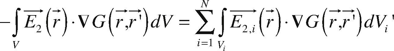
Using the next vector property for each V_i,

and assuming that the resistivity of each body within the half-space (Figure 1), is constant, then ▿′ ^.E→₂ (r→) 0. Thus, we can use the divergence theorem for each V_i and eq. 8 becomes:

This equation should be applied to the whole surface delimitating each immersed body; in our case, we assume the body as a regular prism. Then, the corresponding integral for the case of two contiguous prismatic bodies (b₁,b₂) with a common surface, is:

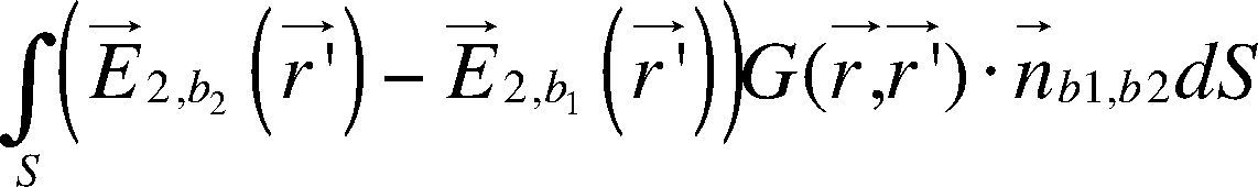
Where n→12 is the unit normal vector of the surfaces (1, 2) between the two bodies.

The boundary conditions allow to define:

where σ_S(r→′) is the density surface charges and ¿₀ is the free-space electrical permittivity.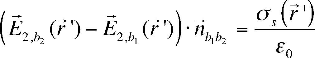

Taking into account the equations (10 to 13), the electric potential (eq. 7) is rewritten as:

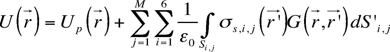
Where number 6 denotes the total number of surfaces of one prismatic body and M the number of bodies within the half-space, this eq. constitutes the SIM.

Eskola (1992) has obtained an expression similar to equation (14) using different analytical approach, under the same type of hypothesis.

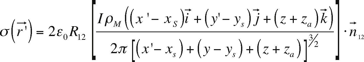
However, a problem to solve is to know σ (r→ ′) (the density surface charges) for each surface of the each prismatic body. Kaufman (1992) expressed σ (r→ ′) for two contiguous surfaces as:

where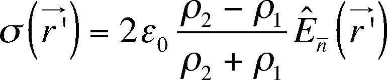

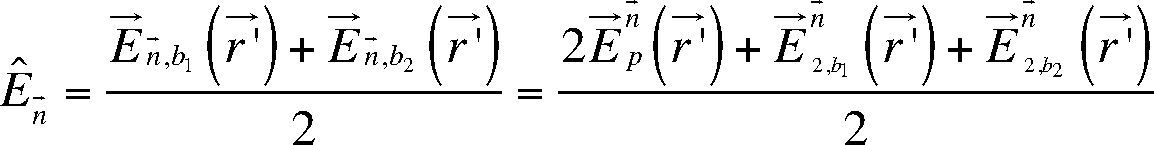
If we neglect the normal electrical secondary field ld in expression (16), i.e.E→n→_{2,b1 (}r→₎ and, E→n→_{2,b2 (}r→₎ then the equation (15) becomes:

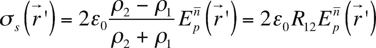
Where, R₁₂, is the reflectivity coefficient between surfaces. This expression is the approximation of the induced surface electric charge and it is equivalent to the so-called “weak scattering problem”.

Numerical Approach

Equations (6 and 14) are expressed in arbitrary coordinate systems with a fixed origin. However, to solve the corresponding integrals we redefine the origin of the coordinate system at the middle point of the prismatic body; that is the “local coordinate system”. The transformation between both coordinate systems will be defined as follows: Assuming P an arbitrary point in the space, its position vector in terms of the global coordinates system is r→ and r→ ′ is its position vector in terms of the local coordinate system. Consequently, the relationship between the origins for both systems is defined by r→_a (see Figure 2), that is:

where r→′ = (x′, y′,z′), r→_a = (x_a, y_b,z_c), and r→=(x, y, z.)

Figure 2.

Relationship between two coordinate systems: global, refers to the external coordinates a n d local, that it is centered at the origin of the immersed resistive body r→=r→′+r→_a.

Assuming isolated heterogeneous bodies immersed in a half space, let us introduce the resistivity contrast as ρ = ρ_c-ρ_m, where ρ_m is the resistivity of the half-space and ρ_c is the resistivity of the immersed body.

Then, by applying equation (6) for a quadrupole array, that is to a vertical electric sounding (VES) (where electrodes are usually named: A, B, N, M, A and B indicate current electrodes and M and N reception electrodes), the potential UsNM associated with a point source electrode can be expressed as eq. (19). This equation also assumes the concept of additive potential sources (Orellana, 1972):

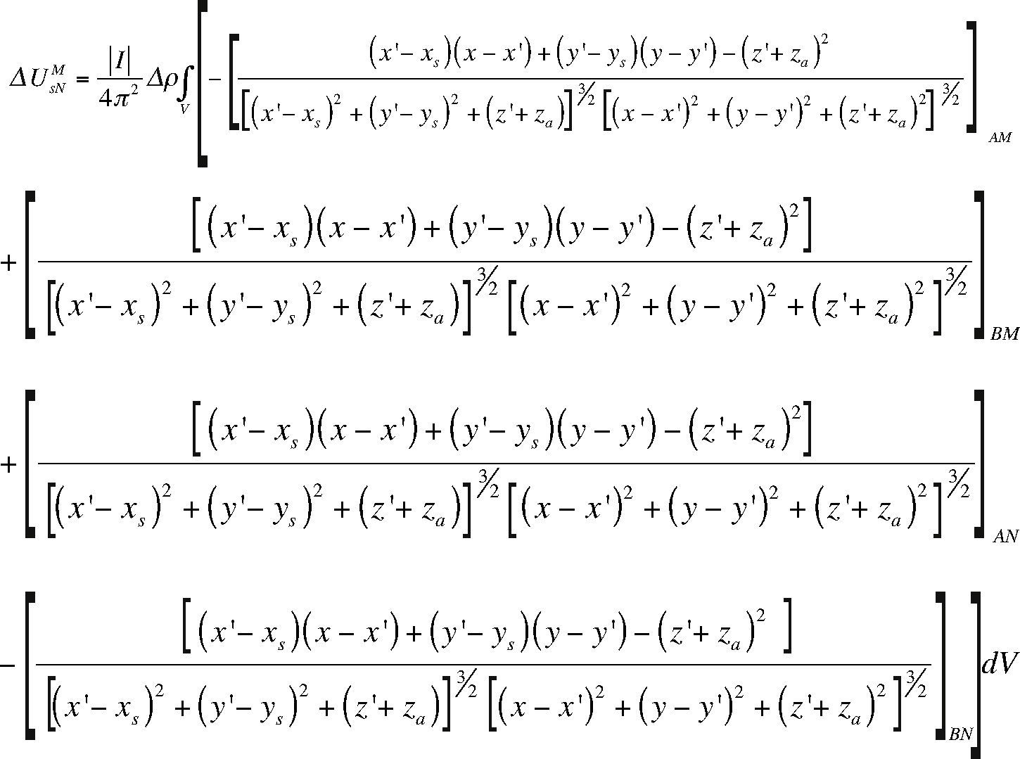
This equation allows us to compute the secondary electric potential by the volume integral method, VIM.

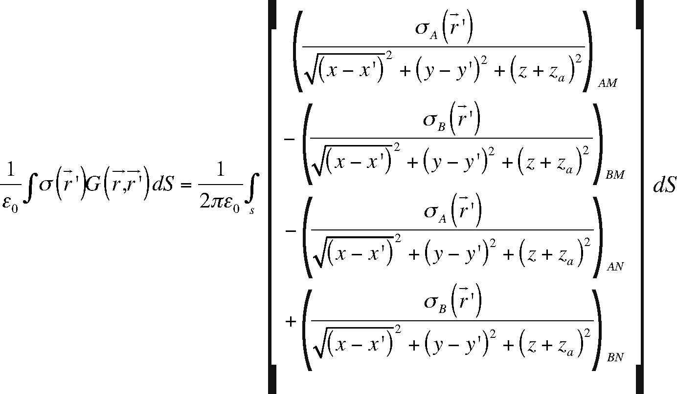
In the eq. 14, SIM, the density surface charges expressed in terms of the local coordinates system is:

By substituting equation (20) in equation (14), the contribution of each surface of the immersed body, to the secondary potential field for the same quadrupole array, is expressed as:

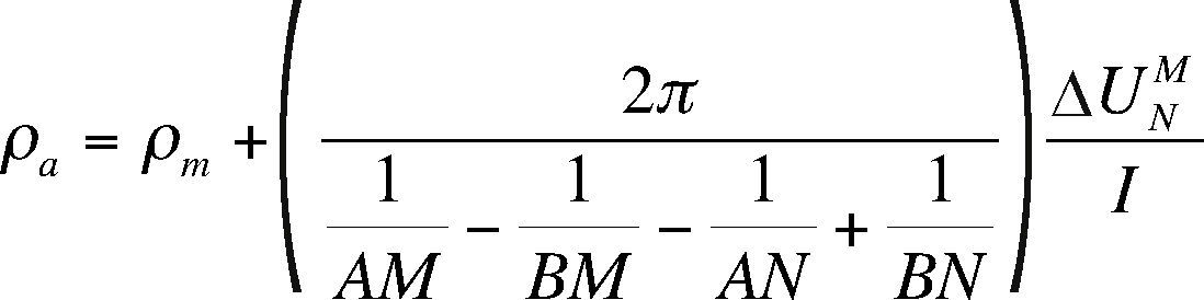
Then the apparent resistivity ρ_a can be expressed as:

To solve the integrals involved in equations (19 and 21) (VIM and SIM, respectively) we use the Gauss-Legendre Quadrature, by using the subroutines QGAUS and DQDAGI, that are in-cluded in the IMLS Fortran numerical libraries (Meissner, 1995; Press et al., 1992). DQDAGI subroutine makes use of Gauss-Kronrod approximation with 21 points, and by using an e-algorithm (Piessens et al., 1983), these integrals can be estimated even when the ending interval is a singularity.

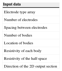
The computational program developed in this work computes the apparent resistivity profile for 3D inmersed bodies, by entering the data listed in table 1. The output data are the apparent resistivity values in an array that corresponds to a resistivity pseudo-section cutting the half-space in the input direction.

Table 1.

Required data in the computational program to computes the apparent resistivity.

Input data
Electrode type array
Number of electrodes
Spacing between electrodes
Number of bodies
Location of bodies
Resistivity of each body
Resistivity of the half-space
Direction of the 2D output section

Synthetic examples

In order to illustrate the validity of the VIM and SIM developed in this work, we studied some synthetic examples and compared them to results obtained by others authors.

A stratified media, with three layers of different resistivities, constitutes the first example (Figure 3a). One case considers a middle conductor layer: 100, 10, 100 ohm-m (Figures 3b); and the other case considers a middle resistive layer: 10, 100, 10 ohm-m (Figure 3c). The results of the SIM model for a dipole-dipole array are compared (Figures 3b and 3c) to those results obtained by applying the algorithm based on the adaptative digital filtering proposed by Anderson (1979), which uses Hankel transforms. This comparison shows coincidences in the computed resistivity values at the subsurface assignation points corresponding to an electrodic separation of a = 1m, and until the level n = 14; however, after level n = 15 the results show differences between values (each level n corresponds to 0.5 m), because the computed induced charge by SIM is a poor approximation. It is important to point out that SIM is one method that needs to model closed bodies and the middle layer was considered as a body of 400 by 400 m and thickness of T = 2.5 m, the depth D = 5 m this assumption involves numerical errors that could explain the enlargement of the differences between both methods at depth (for levels n > 15 and depth > 10.5 m). But also it is important to point out the assumption of weak scattering concerns the use of Born approximation (Guozhong and Torres-Verdín, 2006) and this is also a contribution in those discrepancies, as it was signaled by Zhdanov and Fang (1996), the Born approximation produces curves of the correct shape but incorrect magnitude. In summary, we can conclude the approximation with SIM is good enough.

Figure 3.

a) Synthetic example assuming a stratified half-space of three layers with D = 5 m and T = 2.5 m. The log-log plot shows the comparison between the SIM and the Anderson filter (Anderson, 1979) using two different contrasts of resistivities: b) a middle conductive layer with ρ_m = 100 Ω_m, ρ_l=10 Ω_m and c) a middle resistive stratum with ρ_m = 10 Ω_m, ρ_l=100 Ω_m.

The second example consists of a 3D homogeneous half-space, with ρ_m = 100 ohm-m, and one conductor immersed prismatic body, of ρ_c = 20 ohm-m (Figure 4). The results of VIM method (Figure 5a) shows differences between 3 and 21 ohm-m in the lower values region compared to those computed by Pridmore (1978); while the SIM modeling of a dipoledipole array over the prism are compared (Figure 5b) to those obtained by Tsourlos and Ogilvy (1999). As it is observed, the differences between values are within 1 and 10 ohm-m. In contrast (Figure 5d), and only rise up to 14 ohm-m compared to those obtained by Tsourlos and Ogilvy (1999), Figure 5c. In spite of the differences depicted between the results of SIM and VIM, the results are good enough since the computed resistivity values do not exceed 15 ohm-m (Figures 5a and 5b). That is about 18% of the resistivity contrast between body and half-space.

Figure 4.

The schematic model shows a 3D body, ρ_c = 20 Ω_m, immersed in a homogeneous half-space ρ_m = 100 Ω_m. a/2 is the depth to the top of the body, 2a is the longitude of all sides of the cube, and a is the inter-electrode separation. Distance along the profile is x-coordinate (meters) and z-coordinate designates the positive depth (meters).

Figure 5.

Comparison between results of the second example, constituted by the conductor immersed prismatic body shown in fig. 4, a) the results of the VIM model, b) the results of the SIM model, and those already published c) Tsourlos and Ogilvy (1999), and d) Pridmore (1978).

The third example showed in Figure 6a, is constituted by the synthetic example published by Perez-Flores et al. (2001) with 4 immersed bodies of constant resistivity, ρ_c = 20 ohm-m. This model is based on a volume integral scheme (Perez-Flores et al., 2001) and it is similar to the hypothesis of the VIM proposed here. The comparison between SIM and model shows similar results (Figure 6b). Also, the VIM shows quite the same data for this particular case (not showed in figure); however, for general cases, we would expect bigger differences from VIM results. A possible explanation is that the electrode separation is smaller than the dimensions of the bodies.

Figure 6.

Third synthetic example constituted by (a) 4 immersed 3D bodies ρ_c = 20 Ω_m in a homogeneous half space, b) The results of the SIM model, c) the results published by Flores et al. (2001).

The fourth example presented consists of two conductive bodies (Figure 7) of ρ_c = 20 ohm-m, immersed in a homogeneous half-space of ρ_m = 100 ohm-m. The bodies have the same dimensions, 10 m thick (T, in the z direction), 10 m long (L, in the x direction) and 10 m width (W, in the y direction) and both are located at 2.5 m depth (D). This example is proposed just to show the interaction between bodies by changing the separation between them, with two possibilities: closer and distant (far) bodies, with S equal to 6 m and 40 m respectively. We assume a dipole-dipole array consisting of 31 electrodes, with a 5 m distance between them. Figure 8 shows the results obtained with SIM and VIM for the case with S = 6 m. The apparent resistivity values with SIM are those expected for the bodies. In contrast, VIM's resistivity values are bigger than those expected. It is important to point out that we obtain two minimum resistivities in the location corresponding to the bodies, as we expect, those anomalies in resistivities correspond to the bodies. However, it is also observed a third anomaly at the center of the resistivity image that corresponds to a numerical feature, of a lower resistivity value. Figure 9 shows results for the case S =40 m, they are similar to those obtained for isolate bodies (Figure 6). As well as previous case, it is also observed a third anomaly at the center of the resistivity image that corresponds to a numerical feature.

Figure 7.

The schematic model shows a homogeneous half-space (ρ_m) and two immersed bodies of constant resistivity ρ_c. D is depth from soil to the top of the bodies (a/2), S is the horizontal distance between bodies, (T) high of bodies, (W) wide in y direction and (L) large in x direction, and a is the inter-electrodic separation.

Figure 8.

Pseudo-section model obtained for the fourth example (figure 7), with ρ_c = 20 Ω_m and ρ_m = 100 Ω_m. Simulating a dipole-dipole array of 31 electrodes, with a = 5 m. The apparent resistivities were computed for separation between immerse bodies of S = 6 m. a) SIM and b) VIM.

Figure 9.

Pseudo-section model obtained for the same characteristic of the bodies of the fourth example (fig. 7), with ρ_c = 20 Ω_m and ρ_m = 100 Ω_m, but for separation between immerse bodies of S = 40 m, simulating a dipole-dipole array of 31 electrodes, with a = 5 m, a) SIM and b) VIM.

In all the studies cases, we can observe, SIM produces better approach than VIM in computing the electrical potential.

Conclusions

This paper introduces two algorithms for the integral solution of the forward DC geoelectrical problem introduced by Hvozdara and Kaikkonen (1998) with mixed boundary conditions using Green's function. The two types of solutions: volume (VIM) and surface integral methods (SIM) make use of the resistivity contrast between immersed bodies and the homogeneous half- space. These methods also use the concepts of: additive potential sources for immersed bodies, and density surface charges. Both algorithms are not so much demanding on computer time and memory because they do not produce to very large systems of linear equations. This made the methods more accessible for personal computers, quotidian prospecting work and also makes it attractive for educational purposes. In particular could be useful to easily validate the field measurements interpretation.

The algorithms developed here can help in the interpretation of the field data obtained from resistivity profile methods, in two and three dimensions. The advantage of using the integral equation technique is that it is performed for each immersed body in the half space, in contrast to the usual procedure in finite-element and finite-difference methods. In order to find the induced charge, we do not need to define a grid on the surface of the body, due to the fact that we use the density surface charges on each surface.

The conducted tests with synthetic data indicated that both algorithms (SIM and VIM) produced reasonably good results compared to already published results for similar problems, obtained by other algorithms. The synthetic examples allow us to conclude that SIM produces a better approximation of the apparent resistivity values than those based on the volume integral (VIM).

These results are particularly attractive for computation in parallel, because they provide the mode to obtain the forward response for each body in simultaneous way.

Acknowledgements

This study was financed by the PAPIIT- DGAPA-UNAM research projects IN112906 and IN104006.