Psychological barriers in stock market indices: Evidence from four southern European countries

Abstract

In this paper we examine, for the first time, the major stock market indices of Greece, Italy, Portugal, and Spain for indication of psychological barriers at round numbers. Uniformity in the trailing digits of the indices was tested, and regression and GARCH analysis was used to assess the differential impact of being above or below a possible barrier. No evidence of psychological barriers was detected in the Italian stock market. There was weak evidence of barriers in the Iberian stock markets, and a strong indication of psychological barriers in the Greek stock market. Moreover, it is shown here that the relationship between risk and return tends to be weaker at the proximity of round numbers, which poses a challenge to the traditional equilibrium models.

Resumen

En este artículo se examina por primera vez los principales índices bursátiles de Grecia, Italia, Portugal y España en busca de evidencia de barreras psicológicas en números redondos. Hemos probado la uniformidad de la distribución de dígitos de los índices y hemos usado regresiones y análisis GARCH para evaluar el impacto diferencial de estar por encima o por debajo de una posible barrera. No se detectó ninguna evidencia de barreras psicológicas en el mercado bursátil italiano. Existe evidencia poco sólida de barreras en los mercados ibéricos y una fuerte indicación de barreras psicológicas en el mercado griego. Además, se muestra que la relación entre el riesgo y la rentabilidad tiende a ser más débil en la proximidad de los números redondos, lo cual plantea un reto a los modelos de equilibrio tradicionales.

1

Introduction

Market practitioners and journalists often refer to the existence of psychological barriers in stock markets. Many investors believe that round numbers serve as barriers, and that prices may resist crossing these barriers. Moreover, the use of technical analysis is based on the assertion that traders will “jump on the bandwagon” of buying (selling) once the price breaks up (down) through a “psychologically important” level thus suggesting that the crossing of one of these barriers may push the prices up (down) more than otherwise warranted. Frequently used phrases by the business press such as “support level” and “resistance level” imply that, until such time as an important barrier is broken, increases and decreases in the prices may be restrained.

The impact of such kind of psychological barriers in investors’ decisions has been studied since the 1990s for a variety of asset classes, from exchange rates with De Grauwe and Decupere (1992) to stock options with Jang et al. (2015). The evidence of psychological barriers on stock market indices suggests some significant impacts of this phenomenon in the returns and variances in different geographies and periods (e.g., Donaldson and Kim, 1993; Koedijk and Stork, 1994; Cyree et al., 1999; Bahng, 2003).

This article examines the existence of psychological barriers at round numbers in the major stock market indices of four Southern European countries: Greece (FTSE/ATHEX Large Cap), Italy (FTSE MIB), Portugal (PSI 20) and Spain (IBEX 35). To the best of our knowledge, none of these markets has ever been analyzed with this purpose. And their economic significance is not negligible: the four national stock markets accounted in 2012, in aggregate, for about a third of eurozone's GDP and almost a quarter of eurozone's total stock market capitalization (World Bank, 2014).

The anchoring effect, a well-known behavioral bias firstly identified by Tversky and Kahneman (1974), is the main explanation for the existence of psychological barriers in financial markets. Individuals, when performing an estimation in an ambiguous situation, tend to fixate (‘to anchor’) on a salient number even if that number is irrelevant for the estimation. The anchoring on round numbers is important for its great explanatory power of some of the features commonly associated to financial markets. It may help to understand, for example, the excessive price volatility (Westerhoff, 2003), the momentum effect (George and Hwang, 2004), or even the emergence of speculative bubbles (Shiller, 2015).

Of course, behavioral biases are not the only reason why barriers could exist. For example, the fact that option exercise prices also are usually round numbers may be an additional explanation for the phenomenon.

The existence of psychological barriers contradicts the efficient market hypothesis as it points to some level of predictability in stock markets and thus may lead to abnormal risk-adjusted returns. Hence empirical evidence for the existence of psychological barriers is not only of interest to practitioners who are looking for profitable strategies but it also represents a contribution to the literature on market efficiency and on market anomalies.

Our methodology comprises a number of empirical tests. We test for uniformity in the trailing digits of the stock indices and use regression and GARCH analysis to assess the differential impact of being above or below a possible barrier. The results obtained reveal substantial differences in the incidence of psychological barriers on the markets of the sample. In the Italian stock market, it was not detected any evidence of psychological barriers. There is weak evidence of barriers in the Iberian stock markets. Lastly, the Greek stock market is the one with the strongest indications of psychological barriers nearby round numbers. Moreover, we show that the relationship between risk and return tends to be weaker at the proximity of round numbers, especially in short time horizons (up to five days).

This article is organized in as follows. Section 2 reviews the empirical evidence regarding psychological barriers. Section 3 presents the data and methodologies used in this paper. Section 4 presents the empirical results. Section 5 offers conclusions.

2

Previous findings

Donaldson (1990a, 1990b) and De Grauwe and Decupere (1992) were the first to study the phenomenon of psychological barriers and showed that round numbers are indeed of special importance for investors in the stock and in the foreign exchange markets, respectively. From then on, several other studies followed, focusing not only on different geographies and periods, but also on different asset classes, such as bonds, commodities and derivatives.

To date, stock indices have been the target of most research concerning psychological barriers. Donaldson (1990a, 1990b) used both chi-squared tests and regression analysis to test for uniformity in the trailing digits of the Dow Jones Industrial Average (DJIA), the FTSE-100, the TSE, and the Nikkei 225. His findings rejected uniformity for all but the Nikkei index.

Donaldson and Kim (1993) examined the DJIA for the period 1974–1990 using a Monte Carlo experiment and found evidence confirming round numbers (100-levels) as support and resistance levels. Furthermore, they concluded that once such levels were crossed through, the DJIA moved up or down more than usual in what they called a “bandwagon effect”. The same was not true to the less important Wilshire 5000.

Ley and Varian (1994) also studied the DJIA considering a wider interval of time (1952–1993) and confirmed that there were in fact fewer observations around 100-levels. In 98.4% of the tested cases, uniformity in the trailing digits was rejected at the 95% significance level. Additionally, they emphasized the fact that non-uniform distribution of the final digits was not necessarily synonym of price barriers and found no evidence of stock price predictability due to these barriers.

Koedijk and Stork (1994) expanded the research to a number of indices. The authors studied the existence of psychological barriers on the Brussels Stock Index (Belgium), on the FAZ General (Germany), on the Nikkei 225 (Japan) and on the S&P 500 (U.S.) during the period January 1980 to February 1992, while the FTSE-100 (U.K.) was observed from January 1984 to February 1992. They discovered significant indications of psychological barriers’ existence on the FAZ General, the FTSE-100 and the S&P 500, but weak indications on the Brussels Index, and none for the Nikkei 225. As in Ley and Varian (1994), they failed to find evidence supporting the significance of 100-levels in predicting returns. However, this may be due in part to the fact that they did not disaggregate the effects of upward and downward movements through barriers.

De Ceuster et al. (1998) compared the last digits of DJIA, FTSE-100, or the Nikkei 225 with the empirical distribution of a Monte Carlo simulation. They did not find any indication of the existence of psychological barriers on those three indices.

Cyree et al. (1999) showed that the last two digits of the DJIA, the S&P 500, the Financial Times U.K. Actuaries (London) and the DAX are not equally distributed. Prices next to barriers turn up less frequently than prices in a more distant position. The TSE 300, CAC 40, Hang Seng and Nikkei 225 exhibit some significant evidence. They also analyzed the distribution of the returns with regard to expected returns and volatility in a modified GARCH model to conclude that upward movements through barriers tended to have a consistently positive impact on the conditional mean return and also that conditional variance tended to be higher in pre-crossing subperiods and lower in post-crossing subperiods.

More recently, Bahng (2003) applied the methodology of Donaldson and Kim (1993) to analyze seven major Asian indices including South Korea, Taiwan, Hong Kong, Thailand, Malaysia, Singapore, and Indonesia between 1990 and 1999. Their analysis showed that the Taiwanese index did possess price barrier effects and that the price level distributions of the Taiwanese, Indonesian, and Hong Kong indices were explained by quadratic functions.

Dorfleitner and Klein (2009) focused on the DAX 30, the CAC 40, the FTSE-50 and the Euro-zone-related DJ EURO STOXX 50 for different periods until 2003. They found fragile traces of psychological barriers in all indices at the 1000-level. There were also indications of barriers at the 100-level except in the CAC index.

Finally, Jang et al. (2015) considered the 15-min interval historical records of the S&P 500 Index from July 8, 2011 to January 19, 2012, and found significant evidence of psychological barriers at each 100 level. Moreover, the authors suggested a new model that incorporates the impact of those barriers and compared the model's empirical performance with respect to the Black–Scholes and constant elasticity of variance models.

Other studies concerning psychological barriers in stock markets are also related to our analysis. It is the case of those articles that address the presence of barriers in individual stock prices such as Cai et al. (2007) and Dorfleitner and Klein (2009).

Cai et al. (2007) assessed the existence of psychological barriers in a total of 1050 A-shares and 100 B-shares from both the Shanghai Stock Exchange and the Shenzhen Stock Exchange during June 2002. A range of measures for price resistance showed the digits 0 and 5 to be significant resistance points in the A-share market. No resistance point was found in the Shanghai B-share market, although digit 0 has had the highest level of resistance compared to others.

Dorfleitner and Klein (2009) analyzed eight major stocks from the German DAX 30 over the period May 1996–June 2003. The prices were examined with respect to the frequency with which they lied within a certain band around the barrier. In addition, they studied barrier's influence on intraday variances and the daily trading volume. Overall, the authors were not able to identify a systematic and consistent pattern at barriers.

Different studies concluded that price barriers or at least significant deviations from uniformity also exist in other asset classes such as exchange rates (De Grauwe and Decupere, 1992), bonds (Burke, 2001), commodities (Aggarwal and Lucey, 2007) and derivatives (Schwartz et al., 2004; Chen and Tai, 2011; Jang et al., 2015; Dowling et al., 2016). Overall, evidence of price barriers in various asset classes seems to be fairly robust.

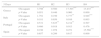
3

Data and methodology

3.1

Data

The examination window for each of the stock market indices under study is presented in Table 1. Starting dates are different since we used the data pertaining each index since its inception. All the data were retrieved from Thomson Reuters Datastream. Summary statistics on the stock prices are presented in Table 2 where it can be seen that the measures of skewness and, especially, kurtosis are in general inconsistent with normality.

Table 1.

Data used in the study.

Country	Stock index	Starting date	Ending date
Greece	FTSE/ATHEX Large Cap	September 23rd, 1997	December 31, 2013
Italy	FTSE MIB	December 31st, 1997
Portugal	PSI 20	December 31st, 1992
Spain	IBEX 35	January 5th, 1987

Table 2.

Summary statistics on stock prices data series.

Country	N	Return series				Level series
		Mean	Std. dev.	Skewness	Kurtosis	Maximum	Minimum
Greece	4245	−0.000002	0.001784	0.98993	37.9344	3301.69	169.88
Italy	4174	0.000000	0.000032	0.11526	11.8689	50,108.56	12,362.51
Portugal	5478	0.000002	0.000071	−0.16431	13.5654	14,822.59	2917.56
Spain	7041	0.000003	0.000126	−0.05759	22.3159	15,945.70	1873.58

3.2

Methodology

3.2.1

Definition of barriers

Following Brock et al. (1992) and Dorfleitner and Klein (2009), we will use the so-called band technique and barriers will thus be defined as a certain range around the actual barrier. The main reason is that market participants will most certainly become active at a certain level before the index touches a round price level. Considering an index level of 100, for instance, over-excitement is expected to begin for instance at 99 or 101, or even at 95 or 105. Barriers will thus be defined as multiples of the lth power of ten, with intervals with an absolute length of 2% and 5% of the corresponding power of ten as barriers. These intervals are conventionally used in the literature about psychological barriers. Formally, we may consider four possible barrier bands:

M100: Barrier level l = 3 (1000 s)	980-20; 950-50
M10: Barrier level l = 2 (100 s)	98-02; 95-05
M1: Barrier level l = 1 (10 s)	9.8-0.2; 9.5-0.5
M0.1: Barrier level l = 0 (1 s).	0.98-0.02; 0.95-0.05

3.2.2

M-values

M-values refer to the last digits in the integer portion of the indices under analysis. Initially used by Donaldson and Kim (1993), M-values considered potential barriers at the levels …, 300, 400, …, 3400, 3500, i.e. at:

Later, De Ceuster et al. (1998) claimed that this definition was too narrow because the series was not multiplicatively regenerative, resulting, for instance, on 3400 being considered a barrier, whereas 340 would not. Additionally, the authors claimed that, as defined by Eq. (1), the gap between barriers would tend to zero as the price series increased, disrupting the intuitive appeal of a psychological barrier. Thus, one should also consider the possibility of barriers at the levels …, 10, 20, …, 100, 200, …, 1000, 2000, …, i.e. at:

and, on the other hand, at the levels …, 10, 11, …, 100, 110, …, 1000, 1100, …, i.e. at:

M-values would then be defined according to these barriers. For barriers at the levels defined in Eq. (1), M-values would be the pair of digits preceding the decimal point:

where P_t is the integer part of P_t and mod 100 refers to the reduction modulo 100. For barriers at the levels defined by Eqs. (2) and (3), the M-values would be defined respectively as the second and third and the third and fourth significant digits. Formally,

where logarithms are to base 10. In practical terms, if P_t = 1234.56, then Mta=34. At this level, barriers should appear when Mta=100. Additionally, Mtb=23 and Mtc=12.

3.2.3

Uniformity test

Having computed the M-values, the next step consists of examining the uniformity of their distribution. Following Aggarwal and Lucey (2007), this will be done through a Kolmogrov–Smirnov Z-statistic test. Thus we will be testing H0: uniformity of the M-values distribution against H1: non-uniformity of the M-values distribution.

It is important to emphasize that the rejection of uniformity might suggest the existence of significant psychological barriers but it is not in itself sufficient to prove the existence of psychological barriers. Ley and Varian (1994) showed that the last digits of the Dow Jones Industrial Average were in fact not uniformly distributed and even appeared to exhibit certain patterns, but the returns conditional on the digit realization were still significantly random. Additionally, De Ceuster et al. (1998) noted that as a series grows without limit and the intervals between barriers become wider, the theoretical distribution of digits and the respective frequency of occurrence are no longer uniform.

3.2.4

Barrier tests

Barrier tests are used to assess whether observations are less frequent near barriers than it would be expected considering a uniform distribution. The existence of a psychological barrier implies we will observe a significantly lower closing price frequency within an interval around the barrier (Donaldson and Kim, 1993; Ley and Varian, 1994). Therefore, the objective of the barrier tests is to investigate the influence of round numbers in the non-uniform distribution of M-values. We will use two types of barrier tests: the barrier proximity test and the barrier hump test.

3.2.4.1

Barrier proximity test

This test examines the frequency of observations, f(M), near potential barriers and will be performed according to Eq. (7).

The dummy variable will take the value of unity when the index is at the supposed barrier and zero elsewhere. As it was mentioned in Section 3.2.1, this barrier will not be strictly considered as an exact number but also as a number of different specific intervals, namely with an absolute length of 2% and 5% of the corresponding power of ten as barriers. The null hypothesis of no barriers will thus imply that β equals zero, while β is expected to be negative and significant in the presence of barriers as a result of lower frequency of M-values at these levels.

3.2.4.2

Barrier hump test

The second barrier test will examine not just the tails of frequency distribution near the potential barriers, but the entire shape of the distribution. It is thus necessary to define the alternative shape that the distribution should have in the presence of barriers (Donaldson and Kim, 1993; Aggarwal and Lucey, 2007). Bertola and Caballero (1992), who analyzed the behavior of exchange rates in the presence of target zones imposed by forward-looking agents, suggest that a hump-shape is an appropriate alternative for the distribution of observations.

The test to examine this possibility will follow Eq. (8), in which the frequency of observation of each M-value is regressed on the M-value itself and on its square.

Under the null hypothesis of no barriers γ is expected to be zero, whereas the presence of barriers should result in γ being negative and significant.

3.2.5

Conditional effect tests

The rejection of uniformity on the observations of M-values is not sufficient to prove the existence of psychological barriers (Ley and Varian, 1994). Therefore, it is necessary to analyze the dynamics of the returns series around these barriers, namely regarding mean and variance in order to examine the differential effect on returns due to prices being near a barrier, and whether these barriers were being approached on an upward or on a downward movement (Cyree et al., 1999; Aggarwal and Lucey, 2007).

Accordingly, we will thus define four regimes around barriers: BD for the five days before prices reaching a barrier on a downward movement, AD for the five days after prices crossing a barrier on a downward movement, and BU and AU for the five days respectively before and after prices breaching a barrier on an upward movement. These dummy variables will take the value of unity for the days noted and zero otherwise. To examine the robustness of the results to the assumption that the regime should last for five days, we will also consider a window of 10 days as in Cyree et al. (1999). In the absence of barriers, we expect the coefficients on the indicator variables in the mean equation to be non-significantly different from zero.

Following Aggarwal and Lucey (2007), we started with an OLS estimation of Eq. (9) but heteroscedasticity and autocorrelation were clearly present across our database. Therefore, the full analysis of the effects in the proximity of barriers required us to apply the former test also to the variances. Eq. (10) represents this approach assuming autocorrelation similar to one as in Cyree et al. (1999) and Aggarwal and Lucey (2007). Besides the abovementioned dummy variables it includes a moving average parameter and a GARCH parameter.

The four possible hypotheses to be tested are the following:H1

There is no difference in the conditional mean return before and after a downward crossing of a barrier.

H2

There is no difference in the conditional mean return before and after an upward crossing of a barrier.

H3

There is no difference in conditional variance before and after a downward crossing of a barrier.

H4

There is no difference in the conditional variance before and after an upward crossing of a barrier.

4

Empirical findings

4.1

Uniformity test

Table 3 provides the results of a uniformity test concerning the distribution of digits for the four stock market indices under scrutiny. Overall, there is robust evidence that the M-values do not follow a uniform distribution in three of the four stock markets. Uniformity is clearly rejected for Portugal and Spain at all significance levels. In the case of the Italian market, uniformity is rejected at 5% only in the three lower barrier levels. The rejection of uniformity of the trailing digits is not so strong in the Greek market: at a significance level of 5%, uniformity is rejected only at the highest barrier level.

Table 3.

Kolmogorov–Smirnov test for uniformity of digits.

Country	Statistic	M0.1 (l = 0)	M1 (l = 1)	M10 (l = 2)	M100 (l = 3)
Greece	Kolmogorov (D) – Statistic value (adjusted)	1.278^*	1.201	1.093	5.457^***
	p-Value	0.076	0.112	0.183	0.000
Italy	Kolmogorov (D) – Statistic value (adjusted)	1.721^***	1.637^***	1.560^**	0.860
	p-Value	0.005	0.009	0.015	0.450
Portugal	Kolmogorov (D) – Statistic value (adjusted)	2.322^***	2.529^***	1.629^***	2.067^***
	p-Value	0.000	0.000	0.010	0.000
Spain	Kolmogorov (D) – Statistic value (adjusted)	6.714^***	2.583^***	1.990^***	1.781^***
	p-Value	0.000	0.000	0.001	0.004

The table shows the results of a Kolmogorov–Smirnov test for uniformity. Each test was performed for the daily closing prices of each stock index. D stands for the value of the test statistic while p-value gives the marginal significance of this statistic. H0: uniformity in the distribution of digits, H1: non-uniformity in the distribution of digits.

*

Significance at 10% level.

**

Significance at 5% level.

***

Significance at 1% level.

4.2

Barrier tests

4.2.1

Barrier proximity test

Results for the barrier proximity tests are shown in Tables 4–6 for the intervals mentioned in Sections 3.2.1 and 3.2.4. As referred above, in the presence of a barrier we would expect β to be negative and significant, implying a lower frequency of M-values at these points. Considering a barrier in the exact zero modulo point, evidence in Table 4 shows that only Spain at the 10-level barrier and Greece at 100-level barrier seem to reject the no barrier hypothesis at a statistical significance of 5% and only the latter still rejects it at 1%. If we assume a barrier to be in the interval 98-02, only Greece seems to reject the no barrier hypothesis at the 1000-level barrier at a statistical significance of 1% (see Table 5). Considering the 95-05 interval, Table 6 shows that the no barrier hypothesis is again rejected only for Greece in the same circumstances. All the other series are either not significant or β is not negative. In any case, there are no evidence of psychological barriers around round numbers in the Italian stock market.

Table 4.

Barrier proximity test: strict barrier.

Countries	M0.1 (l = 0)			M1 (l = 1)			M10 (l = 2)			M100 (l = 3)
	β	p-Value	R-square	β	p-Value	R-square	β	p-Value	R-square	β	p-Value	R-square
Greece	−0.002	0.487	0.005	−0.003	0.433	0.006	−0.010^***	0.027	0.049	−0.012	0.129	0.002
Italy	−0.005	0.468	0.005	0.000	0.991	0.000	−0.001	0.848	0.000	−0.005	0.500	0.000
Portugal	−0.010^*	0.064	0.035	−0.005	0.198	0.017	−0.007	0.287	0.012	−0.006	0.232	0.001
Spain	−0.010	0.540	0.004	−0.009^**	0.044	0.041	−0.008	0.152	0.021	−0.001	0.781	0.000

The table shows the results of a regression f(M) = α + βD + ¿, where f(M) stands for the frequency of appearance of the M-values, D is a dummy variable that takes the value of unity when M = 00 and 0 otherwise. Refer to Section 3.2.4 for details.

*

Significance at 10% level.

**

Significance at 5% level.

***

Significance at 1% level.

Table 5.

Barrier proximity test: 98-02 barrier.

Countries	M0.1 (l = 0)			M1 (l = 1)			M10 (l = 2)			M100 (l = 3)
	β	p-Value	R-square	β	p-Value	R-square	β	p-Value	R-square	β	p-Value	R-square
Greece	0.001	0.352	0.009	−0.001	0.535	0.004	0.000	0.920	0.000	−0.005^***	0.000	0.013
Italy	0.002	0.569	0.003	0.003	0.260	0.013	0.000	0.967	0.000	–0.001	0.516	0.000
Portugal	0.001	0.570	0.003	0.001	0.421	0.007	−0.001	0.665	0.002	0.191^***	0.001	0.002
Spain	0.006	0.395	0.007	0.003	0.195	0.017	0.000	0.916	0.000	0.000	0.943	0.000

The table shows the results of a regression f(M) = α + βD + ¿, where f(M) stands for the frequency of appearance of the M-values, D is a dummy variable that takes the value of unity when M = value is in the 98-02 interval and 0 otherwise. Refer to Section 3.2.4 for details.

***

Significance at the 1% level.

Table 6.

Barrier proximity test: 95-05 barrier.

Countries	M0.1 (l = 0)			M1 (l = 1)			M10 (l = 2)			M100 (l = 3)
	β	p-Value	R-square	β	p-Value	R-square	β	p-Value	R-square	β	p-Value	R-square
Greece	0.001	0.441	0.006	−0.001	0.578	0.003	−0.001	0.492	0.005	−0.004^***	0.000	0.021
Italy	0.001	0.625	0.002	0.000	0.790	0.001	−0.002	0.266	0.013	−0.001	0.146	0.002
Portugal	0.000	0.842	0.000	0.000	0.751	0.001	0.000	0.912	0.000	0.002^***	0.002	0.009
Spain	−0.001	0.858	0.000	0.001	0.649	0.002	0.000	0.978	0.000	−0.001	0.256	0.001

The table shows the results of a regression f(M) = α + βD + ¿, where f(M) stands for the frequency of appearance of the M-values, D is a dummy variable that takes the value of unity when M = value is in the 95-05 interval and 0 otherwise. Refer to Section 3.2.4 for details.

***

Significance at the 1% level.

Overall, evidence is scattered as there is no clear pattern regardless of the interval we consider for the barrier with the possible exception of a 1000-level barrier in the Greek stock market. R-squares are significantly low, which is in line with previous studies.

4.2.2

Barrier hump test

Table 7 shows the results for the barrier hump test, which is meant to test the entire shape of the distribution of M-values. Assuming it should follow a hump-shape distribution, we thus expected γ to be negative and significant in the presence of barriers. The results of the barrier hump test confirm the evidence presented previously with the barrier proximity tests. Again, it is the Greek stock market that stands out: it is the only market that exhibits a persistent barrier, namely at the 1000-level barrier, at a statistically significant level of 1%.

Table 7.

Barrier hump test.

Countries	M0.1 (l = 0)			M1 (l = 1)			M10 (l = 2)			M100 (l = 3)
	γ	p-Value	R-square	γ	p-Value	R-square	γ	p-Value	R-square	γ	p-Value	R-square
Greece	2.20E−07	0.616	0.003	−1.78E−07	0.746	0.002	−2.54E−07	0.683	0.003	−1.00E−08^***	0.005	0.017
Italy	3.20E−07	0.705	0.001	2.30E−07	0.739	0.005	−3.60E−07	0.569	0.009	−4.00E−09	0.192	0.002
Portugal	5.40E−08	0.941	0.004	1.50E−07	0.758	0.015	1.60E−07	0.850	0.001	9.00E−09^***	0.000	0.021
Spain	−4.70E−08	0.983	0.007	3.00E−07	0.612	0.011	−8.00E−08	0.916	0.003	0.00E+00	0.924	0.000

The table shows the results of a regression f(M) = α + φM + γM² + η, where f(M), the frequency of appearance of each M-values, is regressed on M, the M-value itself, and M², its square.

***

Significance at the 1% level.

Overall, from the results presented so far it is possible to discern substantial differences in the incidence of psychological barriers on the markets of the sample. In the Italian stock market, it was not detected any evidence of psychological barriers. In the case of the Iberian stock markets, there is weak evidence of barriers at low levels (1-level barrier and 10-level barrier). Lastly, the Greek stock market is the one with the strongest indications of psychological barriers nearby round numbers. A highly significant barrier was detected at the highest level (1000-level barrier).

4.2.3

Conditional effects test

Assuming the existence of psychological barriers, we expected the dynamics of return series to be different around these points. In fact, results in Table 8 provide some interesting evidence of mean effects around barriers as it is observed, on one hand, that stock market returns in all four markets tend to be significantly higher when a barrier is to be crossed in an upward movement. On the other hand, the coefficients of BD and AD are negative and significant for all indices which means that stock market return tend to be significantly lower in the proximity of a barrier when that barrier is to be crossed on a downward movement. These pattern of conditional effects is similar to the one obtained by Cyree et al. (1999).

Table 8.

GARCH analysis: mean equation (5 days).

5 Days		β1	BD	AD	BU	AU
Greece	Coefficient	1.93E−05^***	−2.50E−04^***	−2.00E−04^***	2.31E−04^***	1.18E−04^***
	p-Value	0.001	0.000	0.000	0.000	0.003
Italy	Coefficient	1.75E−07	−4.88E−06^***	−5.22E−06^***	5.12E−06^***	4.25E−06^***
	p-Value	0.568	0.000	0.000	0.000	0.000
Portugal	Coefficient	2.77E−06^***	−2.69E−05^***	−1.81E−05^***	1.95E−05^***	2.18E−05^***
	p-Value	0.000	0.000	0.000	0.000	0.000
Spain	Coefficient	3.60E−06^***	−2.67E−05^***	−2.29E−05^***	2.11E−05^***	1.97E−05^***
	p-Value	0.000	0.000	0.000	0.000	0.000

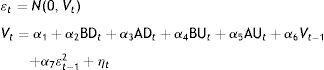
The table shows the results of the mean equation of a GARCH estimation of the form R_t = β₁ + β₂BD + β₃AD + β₄BU + β₅AU + ¿_t; ¿_t ∼ N(0, V_t); Vt=α1+α2BD+α3AD+α4BU+α5AU+α6Vt−1+α7εt−12+ηt. BD, AD, BU and AU are dummy variables. BD takes the value 1 in the 5 days before crossing a barrier on a downward movement and zero otherwise, whereas AD is for the 5 days after the same event. BU is for the 5 days before crossing a barrier from below, while AU is 1 in the 5 days after the same upward crossing. V_t−1 refers to the moving average parameter and εt−12 stands for the GARCH parameter.

***

Significance at the 1% level.

In order to provide some evidence of the robustness of these findings, we estimate the same model with a time window of 10 days. The results are presented in Table 9 and are very similar, both in magnitude and significance, to those presented in Table 8.

Table 9.

GARCH analysis: mean equation (10 days).

10 Days		β1	BD	AD	BU	AU
Greece	Coefficient	1.60E−05^***	−1.70E−04^***	−1.50E−04^***	1.56E−04^***	1.15E−04^***
	p-Value	0.008	0.000	0.000	0.000	0.002
Italy	Coefficient	8.05E−08	−3.06E−06^***	−3.41E−06^***	3.65E−06^***	2.58E−06^***
	p-Value	0.858	0.000	0.000	0.000	0.000
Portugal	Coefficient	2.66E−06^***	−1.89E−05^***	−1.44E−05^***	1.67E−05^***	1.35E−05^***
	p-Value	0.000	0.000	0.000	0.000	0.000
Spain	Coefficient	6.13E−06^***	−2.49E−05^***	−1.65E−05^***	1.23E−05^***	2.15E−05^***
	p-Value	0.000	0.000	0.000	0.000	0.000

The table shows the results of the mean equation of a GARCH estimation of the form R_t = β₁ + β₂BD + β₃AD + β₄BU + β₅AU + ¿_t; ¿_t ∼ N(0, V_t); Vt=α1+α2BD+α3AD+α4BU+α5AU+α6Vt−1+α7εt−12+ηt. BD, AD, BU and AU are dummy variables. BD takes the value 1 in the 10 days before crossing a barrier on a downward movement and zero otherwise, whereas AD is for the 10 days after the same event. BU is for the 10 days before crossing a barrier from below, while AU is 1 in the 10 days after the same upward crossing. V_t−1 refers to the moving average parameter and εt−12 stands for the GARCH parameter.

***

Significance at the 1% level.

Table 10 contains results for the conditional variance equation. The constant is positive and significant for all indices. All coefficients of the lagged squared residuals are positive and significant at the 1% level pointing out to an increase in conditional variance coincident with higher residuals from the previous period. The GARCH term in the conditional variance is positive and significant, suggesting significant GARCH effects around barriers. The GARCH term corresponding to the Spanish market is closer to one which indicates a higher level of volatility persistence. The volatility persistence in Spain, Italy and Portugal is quite higher than Cyree et al. (1999) have found in other European stock markets. The variance effects are particularly evident before an upward movement through a barrier: the coefficient of BU in the variance equation is negative and statistically significant in all the markets under study. This indicates that the markets tend to calm before having risen through a barrier. This is in sharp contradiction with the results obtained by Cyree et al. (1999) according to which, in most cases, markets tend to be more volatile before crossing a barrier in an upward movement. In the pre-crossing period but in the case of a downward movement, the results are heterogeneous: Italy and Portugal have non-significant results whereas the coefficients corresponding to the Greek market and to the Spanish market are significantly positive and significantly negative, respectively.

Table 10.

GARCH analysis: variance equation (5 days).

5 Days		α1	εt−12	Vt−1	BD	AD	BU	AU
Greece	Coefficient	4.00E−09^***	0.2051^***	0.7983^***	4.30E−08^***	−1.40E−08^**	−2.00E−08^***	8.00E−09
	p-Value	0.000	0.000	0.000	0.000	0.038	0.000	0.219
Italy	Coefficient	2.60E−12^***	0.1073^***	0.8948^***	−2.60E−12	9.50E−12^***	−7.80E−12^***	3.00E−13
	p-Value	0.000	0.000	0.000	0.222	0.000	0.000	0.877
Portugal	Coefficient	3.64E−11^***	0.125^***	0.8729^***	4.00E−11	1.05E−10^**	−1.10E−10^***	3.82E−11
	p-Value	0.000	0.000	0.000	0.403	0.036	0.000	0.27
Spain	Coefficient	1.90E−11^***	0.0786^***	0.9263^***	−1.00E−10^**	2.00E−10^***	−5.00E−11^*	−8.70E−11^**
	p-Value	0.000	0.000	0.000	0.026	0.000	0.081	0.020

The table shows the results of the variance equation of a GARCH estimation of the form R_t = β₁ + β₂BD + β₃AD + β₄BU + β₅AU + ¿_t; ¿_t ∼ N(0, V_t); Vt=α1+α2BD+α3AD+α4BU+α5AU+α6Vt−1+α7εt−12+ηt. BD, AD, BU and AU are dummy variables. BD takes the value 1 in the 5 days before crossing a barrier on a downward movement and zero otherwise, whereas AD is for the 5 days after the same event. BU is for the 5 days before crossing a barrier from below, while AU is 1 in the 5 days after the same upward crossing. V_t−1 refers to the moving average parameter and εt−12 stands for the GARCH parameter.

*

Significance at 10% level.

**

Significance at 5% level.

***

Significance at 1% level.

The results in the post-crossing period are also somewhat heterogeneous. The Spanish stock market is the only one that exhibits a statistically significant result in the coefficient of AU. The volatility of the all but the Greek market significantly increases after crossing a barrier in a downward movement, a result that is in line with Cyree et al. (1999).

Again, in order to examine the robustness of these findings, we estimate the same model with a time window of 10 days. The results are presented in Table 11. Although the general picture is not totally dissimilar, in this case there are a number of differences that are worth mentioning. Some coefficients, as in the case of the coefficient of BD and of AU, both for the Italian market, become statistically significant at the conventional levels. And other coefficients have their sign reversed or are no longer significant as in the case of the coefficient of BD for the Italian market and of the coefficient of AD for the Greek market. This suggests that in the case of the variance equation the choice of the time window in GARCH analysis of psychological barriers may be of importance.

Table 11.

GARCH analysis: variance equation (10 days).

10 Days		α1	εt−12	Vt−1	BD	AD	BU	AU
Greece	Coefficient	5.00E−10^**	0.0893^**	0.9169^**	1.00E−08^**	4.00E−09	−8.00E−09^**	1.00E−09
	p-Value	0.001	0.000	0.000	0.003	0.338	0.003	0.721
Italy	Coefficient	4.00E−12^**	0.1382^**	0.8549^**	−3.00E−12^**	8.00E−12^**	−5.00E−12^**	1.00E−12^*
	p-Value	0.001	0.000	0.000	0.007	0.000	0.000	0.065
Portugal	Coefficient	4.00E−11^**	0.134^**	0.8648^**	3.00E−11	8.00E−11^**	−6.00E−11^**	2.00E−11
	p-Value	0.000	0.000	0.000	0.169	0.000	0.000	0.323
Spain	Coefficient	1.00E−09^**	0.1904^**	0.7428^**	4.00E−10^**	1.00E−10^*	−1.00E−09^**	−2.00E−10^**
	p-Value	0.000	0.000	0.000	0.000	0.092	0.000	0.000

The table shows the results of the variance equation of a GARCH estimation of the form R_t = β₁ + β₂BD + β₃AD + β₄BU + β₅AU + ¿_t; ¿_t ∼ N(0, V_t); Vt=α1+α2BD+α3AD+α4BU+α5AU+α6Vt−1+α7εt−12+ηt. BD, AD, BU and AU are dummy variables. BD takes the value 1 in the 10 days before crossing a barrier on a downward movement and zero otherwise, whereas AD is for the 10 days after the same event. BU is for the 10 days before crossing a barrier from below, while AU is 1 in the 10 days after the same upward crossing. V_t−1 refers to the moving average parameter and εt−12 stands for the GARCH parameter.

*

Significance at 10% level.

**

Significance at 1% level.

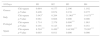
Table 12 shows the test results of the four barrier hypothesis mentioned in Section 3.2.5. If some kind of barrier indeed existed, we would expect that the restraints in terms of mean and variance would be relaxed after the price crossed that barrier. In line with our previous analysis, evidence is weak regarding conditional mean returns associated with indices breaching a barrier. In fact, with the exception of the Greece and Portugal but solely when it comes to the returns on an upward crossing of a barrier and to a downward crossing of a barrier, respectively, there is no significant change in the conditional mean returns in those circumstances.

Table 12.

Barrier hypothesis tests (5 days).

5 Days		H1	H2	H3	H4
Greece	Chi-square	3.798^*	0.580	17.303^***	13.433^***
	p-Value	0.051	0.446	0.000	0.000
Italy	Chi-square	1.791	0.199	5.777^**	8.949^***
	p-Value	0.181	0.656	0.016	0.003
Portugal	Chi-square	0.531	5.635^**	6.214^**	0.507
	p-Value	0.466	0.018	0.013	0.476
Spain	Chi-square	0.198	1.078	0.251	15.568^***
	p-Value	0.657	0.299	0.617	0.000

The table shows the results of a Chi-square test of four different null hypotheses. H1: There is no difference in the conditional mean return before and after a downward crossing of a barrier. H2: There is no difference in the conditional mean return before and after an upward crossing of a barrier. H3: There is no difference in conditional variance before and after a downward crossing of a barrier. H4: There is no difference in the conditional variance before and after an upward crossing of a barrier.

*

Significance at 10% level.

**

Significance at 5% level.

***

Significance at 1% level.

In fact, the first hypothesis, which tested differences in conditional mean returns before and after a downward crossing of a barrier, is only rejected at a 10% level for the Greek case, whereas the second one, which focus on the upward movement, is rejected for Portugal at a 5% statistical level. In both cases, there was a significant increase in the mean return in the post-crossing period.

Following again our previous findings, evidence is more significant regarding the conditional volatility of stock market indices. Regarding the third parameter restriction, which tested the difference in the conditional variance before and after a downward crossing of a barrier, we now find that this difference is statistically significant at least at 10% level for three out of the four markets of the sample (the Spanish market is the exception). Regarding the dynamics of volatility tested in the fourth hypothesis, it can rejected the inexistence of differences in conditional variance before and after an upward breaching of a barrier again for three out of the markets which comprise the sample (the Portuguese stock market is now the exception). In all these cases, the results show a significant increase in variance after crossing the barrier.

When we consider a longer time window, of 10 days, the results are not qualitatively very different, as it can observed in Table 13, below. Nonetheless, there is an increased evidence of significant change in the mean return before and after the crossing of a barrier and a milder evidence, especially regarding the Greek market, of significant changes in conditional variance.

Table 13.

Barrier hypothesis tests (10 days).

10 Days		H1	H2	H3	H4
Greece	Chi-square	0.684	0.177	2.196	1.192
	p-Value	0.408	0.674	0.138	0.275
Italy	Chi-square	3.043^*	0.264	31.065^***	14.875^***
	p-Value	0.081	0.608	0.000	0.000
Portugal	Chi-square	1.714	2.378	9.090^***	1.963
	p-Value	0.191	0.123	0.003	0.161
Spain	Chi-square	8.594^***	6.489^**	144.569^***	79.987^***
	p-Value	0.003	0.011	0.000	0.000

The table shows the results of a Chi-square test of four different null hypotheses. H1: There is no difference in the conditional mean return before and after a downward crossing of a barrier. H2: There is no difference in the conditional mean return before and after an upward crossing of a barrier. H3: There is no difference in conditional variance before and after a downward crossing of a barrier. H4: There is no difference in the conditional variance before and after an upward crossing of a barrier.

*

Significance at 10% level.

**

Significance at 5% level.

***

Significance at 1% level.

Overall, evidence suggests that, although there are no significant effects in terms of returns in stock market indices around barrier points, volatility is in fact significantly affected in most of the markets under scrutiny, especially in the short run (up to five days).

A similar result was obtained by Cyree et al. (1999) for several indices representing developed stock markets. The authors noticed that their result – a simultaneous increase in conditional return and a decrease in conditional variance – appeared to represent an “aberration” in the equilibrium risk–return relationship. As pointed out also by Aggarwal and Lucey (2007), such findings pose some relevant implications for the positive risk–return relationship postulated by the standard financial models. As variance is normally used as a proxy for risk, changes in this parameter should be linked to changes in expected returns. However, our findings suggest that this relationship may be biased in the case of stock market indices near round numbers.

5

Conclusion

Psychological barriers have been found to impact financial markets in different geographies and asset classes. Due to several behavioral biases and the consequent inability to make fully rational decisions, the average market practitioner is often affected, directly or indirectly, by such phenomenon.

Following the most widely used methodologies for studying psychological barriers, we provide new evidence regarding this phenomenon in four Southern European stock markets. Considering an extended sample period, we examined the existence of barriers at round numbers in the major stock market indices of Greece (FTSE/ATHEX Large Cap), Italy (FTSE MIB), Portugal (PSI 20) and Spain (IBEX 35).

In summary, it was possible to distinguish three types of situations regarding the stock markets under scrutiny. In the Italian stock market, it was not detected any evidence of psychological barriers. In the case of the Iberian stock markets, there is weak evidence of barriers at low levels (1-level barrier and 10-level barrier). Lastly, the Greek stock market is the one with the strongest indications of psychological barriers nearby round numbers. A highly significant barrier was detected at the highest level (1000-level barrier). Moreover, it was observed that the stock market returns tended to be significantly higher when a barrier is crossed in an upward movement and significantly lower when a barrier is crossed in a downward movement. Our test for conditional effects also showed that the stock markets suffered some impacts in terms of volatility around barriers.

These findings provide evidence supporting the existence of psychological barriers with respect to index returns. Our results are thus in line with earlier studies (e.g., Koedijk and Stork, 1994; Cyree et al., 1999; Bahng, 2003) and support the claim that technical analysis strategies based on price support and resistances can be profitable, at least in some stock markets. It is also interesting to notice that the markets that are more volatile–in our sample, the Greek market and, to a lesser extent, the Portuguese and Spanish markets – are the ones that exhibit greater indications of psychological barriers.

The implications of the results presented here are somewhat problematic for standard risk–return equilibrium models which predict a positive relationship between these two variables. The findings regarding the barrier hypothesis tests presented in Tables 12 and 13, show that in the markets under analysis there were statistically significant changes in the volatility between the pre-crossing and the post-crossing periods. Changes in variance, as a proxy for risk, should of course be associated with changes in expected returns. However, the contemporaneous changes in the observed returns between those two periods do not seem to be significant in most cases. This lead us to conclude that the relationship between risk and return became weaker around psychological barriers, especially during short periods of time (up to five days).

The fragility in the relationship between risk and return, both in cross-sectional and in temporal frameworks, has been highlighted by several authors over the last decades. For example, Fama and French (1998, 2004) have shown that, after controlling the data for factors such as the book-to-market and the stock capitalization, the relationship between the observed returns and the beta risk parameter becomes statistically non-significant, if not negative. And more recently, Savor and Wilson (2014) have shown that beta is positively related to average stock returns only on days when macroeconomics news regarding employment, inflation, and interest rate are scheduled to be announced. On the remaining days, beta is unrelated or even negatively related to average returns. The results of our study suggest an additional circumstance where the relationship between risk and return tends to be weaker: in the proximity of psychological barriers (in our case, round numbers).

There is much to be investigated about psychological barriers in financial markets. Further avenues for research may include the adoption of statistical tests based on the assumption that prices follow specific distributions (e.g., the Benford’ Law) and the study of the impact of salient events (e.g., a financial crisis) on the prevalence of price barriers.