


How does the arrival of information affect portfolio choice? What is the value of private information? This work examines the impact of private information in a setting where agents make portfolio decisions. We find that more that quantity of private information, what really matters to answer the above questions is how accurate is that information. Indeed, asset allocation decisions differ among informed and uninformed agents only if the quality of information is good enough. Furthermore, we find that agents endowed with a high accurate signal will invest more than uninformed agents, and the larger its precision, the larger the share allocated to the risk asset. The higher the degree of risk aversion, the higher the monetary value of the information, although not in a monotonic way. We also show that more information is beneficial only when it is of greater quality. When the solutions are interior, the value of information is affected by the precision of the signal, as well as the probability of having a good state but it is not influenced by variables like wealth, risk¿free rate and the level of payoffs. The more precise private information is, the higher the value of that information; and the larger the initial prior of having a high return, the less useful that information is. We find that when the agents have private information, their portfolio choice becomes more sensitive to the arrival of new information, provided the quality of it is good enough. We also show that more information is beneficial only when it is of greater quality. When the solutions are interior, the value of information is affected by the precision of the signal, as well as the probability of having a good state but it is not influenced by variables like wealth, risk free rate and the level of payoffs. The paper shows that the more precise private information, the higher the value of information. Furthermore, the larger the initial prior of having a high return, the less useful the information.
¿Cómo la información privada afecta las decisiones de cartera de inversión? ¿Qué valor tiene ese tipo de información? Este trabajo estudia el impacto de la información privada en la cartera de inversiones y demostramos que no es tanto la cantidad de información privada, sino la calidad de esa información la variable crucial que da respuesta a estas preguntas. De hecho, las decisiones de cartera difieren entre agentes informados y no informados si la precisión de la información es suficientemente alta. Los inversores con información privada de calidad invierten más en carteras arriesgadas que los no informados, y a mayor precisión de la información, mayor el porcentaje de riqueza en activos arriesgados. Igualmente, a mayor grado de aversión al riesgo, mayor el valor monetario de la información, pero la relación es no¿monotónica. También demostramos que la información es beneficiosa si es de calidad. De hecho cuando las soluciones de cartera son interiores, el valor de la información viene afectado por variables como la varianza de la información y la probabilidad de tener un retorno alto, pero no por variables como riqueza, el tipo de interés libre riesgo y los retornos de los activos. A más precisa es la información privada, mayor es el valor de esa información, y a más alta es la probabilidad subjetiva inicial de tener unos retornos altos, menor es el valor de la información privada.
1. Introduction
In the developed world, a large fraction of value added comes from enterprises involved in acquiring, processing and synthesizing information like consulting, forecasting or financial analysis. Moreover, the amount of resources devoted to these knowledge-driven activities is growing over time. However, as Veldkamp (2011) points out, most macroeconomic models focus on goods production instead, forgetting about the analysis of the value added of the flows of information that governs production and investment decisions. Only a small body of research tells us about how information is acquired and how it is processed.
This paper models explicitly how investors process information and explains its consequences for portfolio choice decisions. More concretely, the purpose is to explain the fraction of financial wealth households invest in risky assets, conditional on being a stockholder as well as the value of having a better knowledge about the stock market.
In the real world some agents have private information and process it. The way such information is processed (what we call learning) affects what agents know about future realizations of random variables and thus, their behaviour.
We propose a model of portfolio choice in which agents can invest their wealth in a risky and in a riskless asset. The riskless asset pays a sure return, whereas the return on the risky asset is not perfectly known. In our model, some agents are endowed with signals about the return on the risky asset and update their information using Bayes' law. The acquisition of private information is costly for the agent. On the contrary, the rest of the agents simply have access to public information on the distribution of risky returns. We develop a partial equilibrium framework with agents choosing consumption, saving and portfolio allocations decisions under the two information structures.
We show that for investors facing a choice under uncertainty, greater access to information permits decisions that are better suited to the new conditions. Indeed, when the quality of the signal is high, agents receiving a good (bad) signal invest more (less) in the risky asset than uninformed ones, so that investment becomes very sensitive to the arrival of new information. On the contrary, when the signal is not informative at all, the optimal portfolio choice of informed and uninformed agents is similar. Therefore, what really matters for investors is not the quantity of information being provided, but the quality of that information. Moreover, conditional portfolio shares of stocks are increasing in wealth, and decreasing in transaction costs, which is consistent with the data. The paper also shows that, conditional of receiving a high signal, a better precision induces investors to hold even more stocks and the opposite occurs if the signal is low. Moreover, the average volume of investment is increasing in the precision of the signal.
When we study the value of information, we conclude two important things. First, the paper shows that information is useful only when it is of high quality. Certainly, if portfolio choice is equivalent among all different information structures, information has no value at all. By contrast, information is valuable if observing private information would reverse portfolio choice decisions. Second, when the solutions are interiors we find that the value of having private information increases as the information received is of higher quality and decreases with the initial prior, but variables like wealth, risk-free rate, the level of payoffs is of no relevance in explaining the value of information.
Before turning to our analysis, it is important to place our contribution in the broader context of the literature on endogenous information and portfolio choice.
From the theoretical point of view, Grossman and Stiglitz (1980) build a static model of information acquisition in an endowment economy with a risky asset whose price is determined in equilibrium. Investors acquire a signal or not. Their key results are first, that higher information demand will raise the equilibrium price of the asset. And second, that the value of the signal declines as more investors choose to observe it because the price of the asset contains more information. The authors call this result the "fundamental conflict between the efficiency with which markets spread information and the incentives to acquire information".1 Peress (2004) extends Grossman and Stiglitz (1980) model using information costs to explain why wealthier households invest a larger fraction of their wealth in risky assets without having lower relative risk aversion. The reason is that the value of information increases with the amount invested, whereas its cost does not. This implies that agents with more wealth to invest acquire more information. They consequently purchase an even bigger number of stocks and eventually hold a larger portfolio share. Thus, they do so not because they are relatively less risk averse but because the stock is less risky to them. That is, having a riskier portfolio makes information more valuable for these investors so they acquire more private information. And, a higher precision induces investors to hold even more stocks.
In a similar vein, Hong et al. (2004) consider investors having the possibility to buy a risky and a risk-less asset in a static framework. Their focus is on how stock market participation is influenced by social interaction. They distinguish between social-investors (e.g. those who interact with their neighbours) and non-social ones. Non¿socials face fixed participation costs, but these fixed costs are lower when the participation rate among their peers is higher. The paper predicts higher participation rates among social investors than among "non-socials". Using data from the Health and Retirement Study, the authors also test the hypothesis that the decision to invest or not in the stock market is influenced by social interactions with their neighbours. The data confirm their hypothesis: social investors are 4% more likely to invest in the stock market than non-social ones. Our model is very closely related to Hong et al. (2004) in that we use a similar static portfolio choice setup. However, while Hong et al. (2004) do not introduce any learning technology and all agents have the same information, in our setup agents differ in their information endowments and processing.
From an empirical perspective, new evidence documents the importance of information acquisition for stock ownership (see Bonaparte, 2006; Guiso & Jappelli, 2002; Alessie et al., 2002; Borsch-Supan & Eymann, 2002; King & Leape, 1987, among others). Bonaparte (2006), in an analysis of the Survey of Consumer Finance, shows that wealthier households obtain a higher return on their stocks than less wealthy people due to two factors. On the one hand, wealthy investors employ more productive search efforts than their poorer counterparts. On the other hand, wealthy investors are willing to bear higher financial risk and search in a more intensive way. Also, the existence of participation costs seems to explain why wealth together with households' education determines agents' participation in the stock market (Vissing-Jorgensen, 2004). However, these costs are not enough to explain the different degrees of participation in the stock market (the so-called stockholding puzzle), which suggests that additional factors may be driving this different behaviour.2
The rest of the paper is organized as follows. We introduce the model in Section 2. Next, we solve with the equilibrium, highlighting the different ways through which private information operates. Section 3 studies how welfare interacts with risk aversion. Section 4 analyzes the value of information acquisition. Section 5 concludes the paper. The appendix contains the omitted proofs.
2. The model
The setup is a static model for a representative agent and is based on Hong et al. (2004). In this economy individuals maximize their utility given by
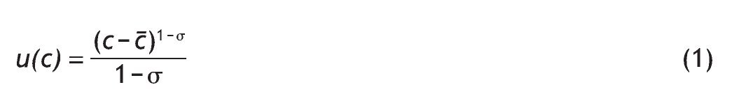
with σ>0. That is, we consider Stone-Geary preferences. These preferences require a minimum level of consumption (c) for the individual, which can be interpreted as a subsistence level in consumption, such that marginal utility goes to infinity if consumption approaches this level (Bertola et al., 2006). This type of preferences exhibit DARA and DRRA if c ≥ c¿.3
Individuals' only source of income is wealth, which can be invested in a risk-less bond paying a sure interest rate of rF, or in a risky asset, that pays r. The return of the risky asset follows a binomial distribution: it pays a high interest rate rH with probability p0, and a low interest rate rL with probability 1 - p0. We assume that rH > r F > rL.
Individuals choose how much of their wealth to invest in the risky asset, h, and how much in the riskless bond, 1 - h. Following a common assumption in the literature on portfolio allocation, the agent is subject to a short-sales constraint, so that the portfolio share must satisfy hÎ [0,1]. Before investing in the stock market, agents pay a fixed entry cost, θ, which is the same for all investors.4
Therefore, the budget constraint of each individual is given by
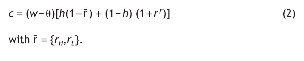
Individuals know the return on the riskless bond, but they do not know the return on the risky asset, only the distribution it follows. Given this information structure, we will compare two alternative scenarios. In one case, individuals will be uninformed, that is, they will use the publicly known distribution on the risky return when deciding their portfolio choice. In the alternative case, individuals will be informed, that is, they will receive a signal on the nature of the risky return. This signal will be used in updating the expected the publicly known distribution on return of the risky asset. Notice that our model does not predict how much information agents will choose to have. Instead, when they are created, some agents receive private information and others do not.
2.1. Uninformed agents
In this section we describe the optimal decision of those agents who do not have access to private information. These agents have a prior probability p0 of receiving a high return, which is publicly known. The objective of investors is to maximize their utility subject to the budget constraint,
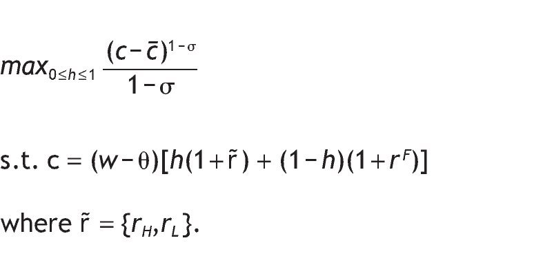
that is, the agent's utility only depends on consumption, and this in turn depends on how much they earn plus interests from his investment decisions. The problem can be simplified to
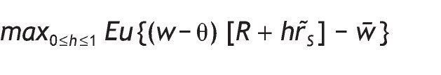
where R = 1 + rF is the gross return on the risk-free asset, and r˜s denotes the excess return on the risky asset. Since the return on the risky asset is random, the individual will maximize their expected utility by simply choosing the proportion of wealth devoted to the risky asset, h.
The F.O.C. for an interior solution can be expressed as follows:
Notice that m'0 > 0, because r˜SH > 0 and r˜SL < 0 (otherwise, if rL > r F everybody would invest in the riskless asset). The optimal proportion of wealth invested in the risky asset in the case of uninformed agents, h*0, is given by
. Finally, the indirect expected utility of an uninformed agent is given by
2.1.1. Comparative statics
One of the advantages of assuming Stone-Geary preferences is that it allows wealth to have a role in determining the optimal portfolio choice. Specifically, h*0 depends positively on the level of wealth
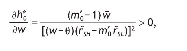
that is, in this model, richer consumers will invest more wealth in the risky asset. This result is consistent with the empirical evidence which shows that wealth is the strongest determinant of market participation: participation rates increase from 3% to 55% from the first to the fifth wealth quintile (Mankiw & Zeldes, 1991). Wachter and Yogo (2010) assume non-homothetic utility over basic and luxury goods, calibrate the model and find that portfolio share rises in wealth, even after controlling for stock market participation and education. They confirm this prediction with household portfolio data from the Survey of Consumer Finances.
Also, h*0 is decreasing in the level of participation costs, θ,
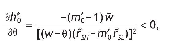
so that the larger the entry cost, the smaller the share of risky asset. There is strong support for the presence of this fixed transaction cost. Vissing¿Jorgensen (2002) finds that a fixed cost of equity market participation as low as $200 would be sufficient to lead to the currently observed rates of non¿participation. Some of these fixed costs may be non-pecuniary, such as the need to educate oneself on how markets work or how to invest. Such costs are likely to vary across individuals, and indeed studies have shown that equity market participation rates increase with the level of education, income, age, and wealth, and that men are more likely to participate than women (Poterba & Samwick, 1997).
2.2. Informed agents
We now turn to the case in which individuals receive a signal on the return of the risky asset. We are interested in measuring the value that private information has on portfolio choice. We will assume that this signal is the same for every individual, so that there is no heterogeneity in this aspect of the model.
2.2.1. Introducing a signal
In the simplest binary model, there are two states of nature (high and low returns, rH and rL, respectively) and informed individuals receive the information with a binary signal. We consider a single signal for each informed agent. The private signal can be high (sH) or low (sL) with probabilities given by the following table:
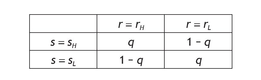
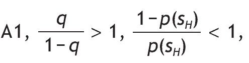
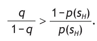
This probability matrix gives us the p(s = si|r = ri) where i = {H,L}. The symmetry does not restrict the generality of the analysis and it simplifies its exposure. Since the signal is symmetric we can either concentrate in the case of qÎ (1/2,1), or we can assume qÎ (0,1/2). We assume that qÎ (1/2,1),

then there is a positive correlation between the signal and the return so that s = sH is interpreted as a good signal because receiving a high signal increases the probability of a high return. Indeed, when q is 1 there is a perfect posiive correlation and the information is perfect, i.e. a perfect signal.5 Finally, when q = 1/2, the signal is not informative at all. The parameter q will be called the precision of the binary signal, for an obvious reason, and it tells us how informative the signal is. Under Assumption A1, the larger the precision q, the more accurate the signal.
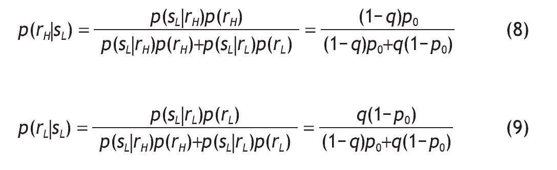
When an informed investor computes the probabilities of high or low returns on the risky asset they take into account the signal they have received. Investors update their probabilities using Bayes' rule. Therefore, conditional on receiving a good signal (s = sH) the updated probabilities become
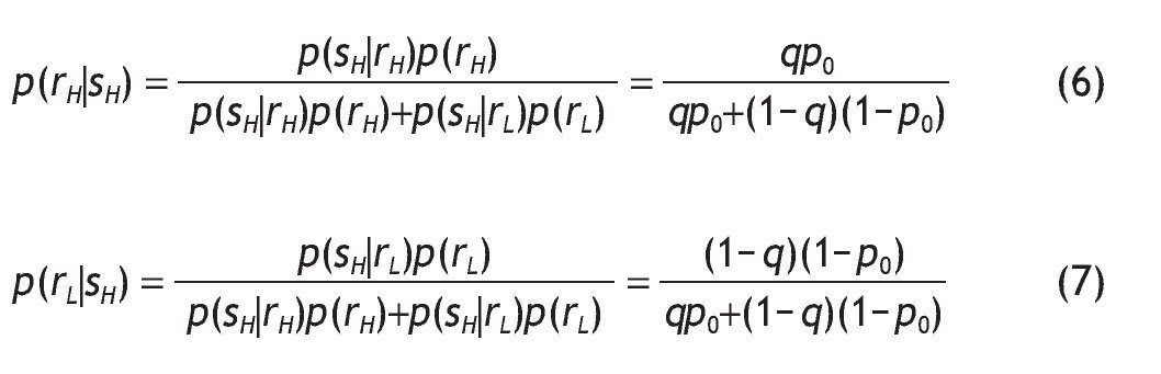
Similarly, conditional on receiving a bad signal (s=s_{L}) we have
Therefore, the probabilities of receiving good and bad signals are

and

The following Lemma summarizes the properties of the conditional probabilities and the probability of having a high signal, sH.
Lemma 1:
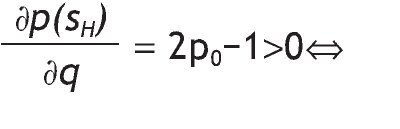
A. If p0 > 1/2, then the probability of receiving a high signal is increasing in q (low signal is decreasing in q). Similarly, if Assumption A1 holds, then the probability of receiving a high signal is increasing in p0 (low signal is decreasing in p0).
B. If p0 > 1/2 and Assumption A1 holds, then the probability of receiving a high signal is larger than the probability of receiving a low signal.
C. If p0 > 1/2 and Assumption A1 holds, then conditional of receiving a high signal, the probability of having a high return is larger than the probability of having a low return, that is, p(rH|sH) > p(rL|sH).
Proof: See Appendix.
The maximization problem of an agent receiving a good signal is given by,
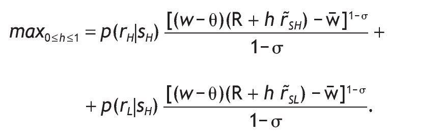
The optimal share allocated to stock is
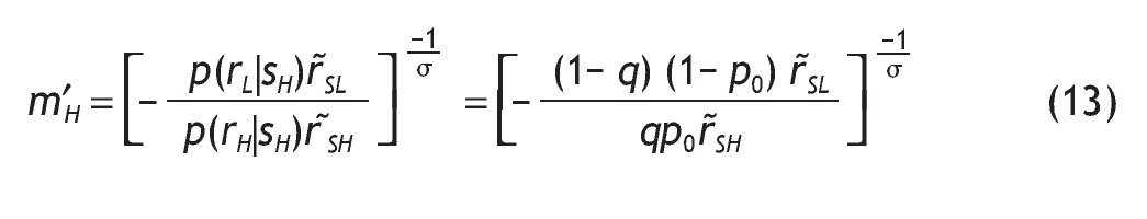
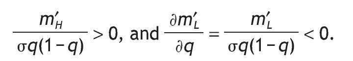
, as defined in the case of uninformed agents. And the corresponding m'H is
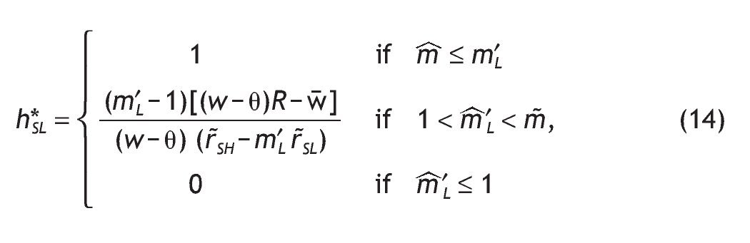
Similarly, for an agent receiving a bad signal, the optimal fraction of wealth in the stock market for this agent is given by
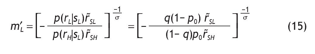
with m'L given by
The following proposition summarizes the composition of the portfolio choice among informed and uninformed investors, emphasizing the role of information in explaining asset allocation decisions.
Proposition 1:
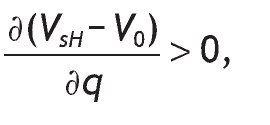
1. Under Assumption A1, the share allocated to the risky asset is larger for agents receiving a high signal than for agents with a low signal. Indeed, comparing portfolio composition of informed versus uninformed investors we obtain:
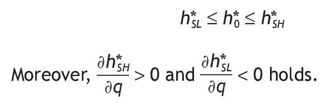
2. If Assumption A1 holds and the signal is perfect, the participation rates of agents endowed with a low signal is zero (i.e. h*SL = 0,) and agents endowed with a high signal would have the maximum exposition to stock market risk (i.e. h*SH = 1).
3. When the signal is very noisy (i.e. q = 1/2), the decision rules about the share of stocks in their portfolios are similar among informed and uninformed investors.
Proof: See Appendix.
This proposition shows several things. First, having private information of high quality becomes a key determinant in explaining asset allocation decisions. This is so because if the information is not accurate enough (i.e. q = 1/2 ) portfolio choice among informed and uninformed investors are similar. However, when the signal is accurate (i.e. q > 1/2) agents informed with a high signal will invest more in the risky asset than those uninformed agents, while agents informed with a bad signal will invest less.6
Moreover, a better precision will increase the proportion of wealth invested in the risky asset with a high signal. This means that accurate and positive information about an asset or company performance may cause to invest more on it. By contrast, if the signal is bad, the proportion of wealth invested in the risky asset will decrease. Consequently, what really matters for investors is not the quantity of information being provided, but the quality of that information. A corroborating evidence for this proposition will be to see how differences in information content creates movements in the proportion of wealth invested in risky assets. We will expect portfolio choice to be very sensitive to the arrival of positive or negative accurate news. Consistent with our story Van Nieuwerburgh and Veldkamp (2009), using data on information choice, show that the home bias in equity holdings arises because home investors know more about home assets.7
Another channel by which information acquisition may affect portfolio choice is through changes in the equilibrium stock return. However, as mentioned above, asset pricing is beyond the scope of this paper.8
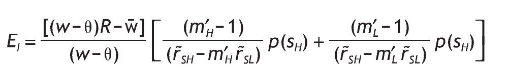
We can analyze some comparative statics for the ex-ante (before the signal is received) average proportion invested in the risky asset, EI, that is,
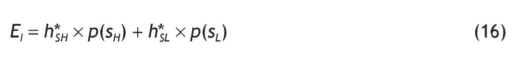
Using the interior solutions and the unconditional probabilities of the signals given by equations (10) and (11),9
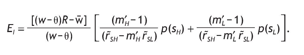
As before, notice that due to the Stone-Geary preferences both wealth and entry costs have a role in the determination of the expected investment in the risky asset. In particular, we have
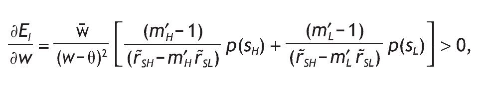
that is, the expected investment in the risky asset is increasing in wealth, so that richer people on average invest more in the risky asset.
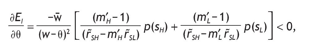
Similarly, the higher the fixed participation cost in the risky asset, the lower the expected investment in the risky asset, i.e.
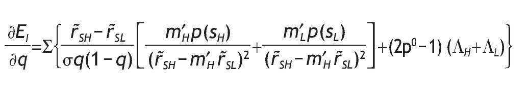
The next proposition analyzes how the variance of the signal affects the average volume of investment. The precision have two opposite effects working in opposite directions. However, as information becomes more accurate, the positive effect due to the larger investment in a risky asset if endowed with a high signal more than compensate the negative effect of decreasing the exposition to stock market risk if endowed with a low signal. The overall effect is to increase the average volume of investment.
Proposition 2: Under Assumption A1 and p0 ≥ 1/2, the average volume of investment in the risky asset increases with the precision of the signal,
Moreover, the average investment in the risky asset with a high signal increases with its precision, and the average volume of investment with a low signal decreases with its precision.
Proof: See Appendix.
3. Welfare and risk
Now we are ready to analyze the welfare effects in terms of wealth of acquiring information. To this end, we will study how information acquisition interacts with the degree of risk aversion.
Welfare contingent on receiving the high signal is
Welfare contingent on receiving the low signal is
And, finally the welfare of an uninformed agent is
As a first approach, let us consider the case of CRRA utility functions, that is, let us set w = 0. This particular case allows us to compute the value of information concerning individuals' welfare, and to compare it with previous studies. Following Eeckhoudt et al. (2005) we compute the monetary value of information, κ, which is defined as
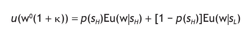
that is, we compute the monetary amount that would leave the individual indifferent between being informed or not and getting the compensation of κ%. The expectations on the right¿hand side of the equation denote the expected utility obtained once a signal has been received, and depending on the realization on such signal.
Figure shows the monetary value of information in percentage terms, κ, as a function of the degree of relative risk aversion, σ.10 We should expect that the higher the degree of risk aversion, the higher the monetary value of the information, thus, the larger κ.11 However, consistent with previous findings (Treich, 1997; Persico, 2000), it is not always the case and, as Figure shows us the value of information depicts a hump-shaped curve as a function of risk aversion. That is, the value of information decreases for relatively high degrees of risk aversion.
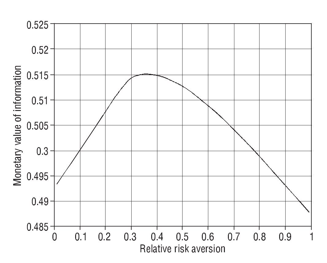
Figure The monetary value of information (κ) in % terms as a function of the degree of relative risk aversion. The CRRA case.
Intuitively, in our simulations, for degrees of risk aversion lower than 0.33 it is optimal for the individual to get the compensation without information. Lower risk aversion increases the amount of risk the individual would be willing to accept by getting information, therefore the prime increases. However, for σ > 0.4, more information increases the risk the individual would optimally put up with, thus reducing the compensation required in the case of no information. That is, higher risk aversion affects positively the value of wealth without information compared to the value of wealth with information. For DRRA utility functions, like the one employed in this paper, the results would be similar qualitatively but change quantitatively, since the proportion of wealth invested in the risky asset, h, depends on the minimum level of wealth, w.
4. The value of information and logarithmic utility
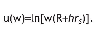
In this section we examine the effect of information on welfare. To this end, we fix the degree of risk aversion and examine the value of information for the decision maker assuming the logarithmic utility function. Following Veldkamp (2011, chapter 7), we define the value of information as the difference of the utility functions with and without the signal, for a given set of parameters values.
Imagine there is no fixed cost and w=0,12 thus the utility function takes the form
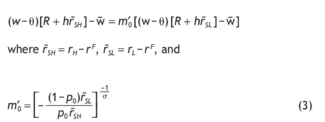
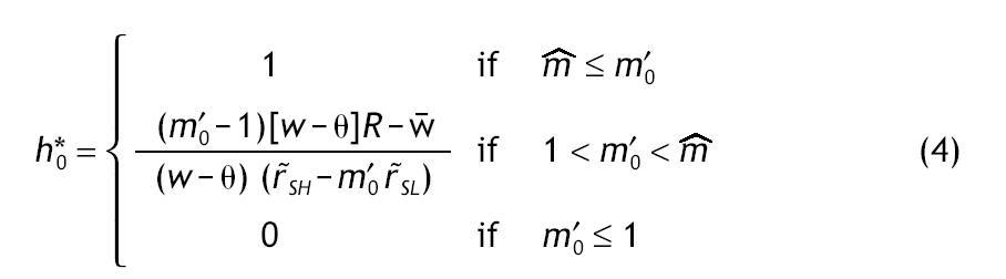
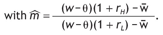
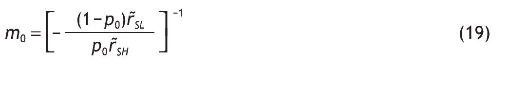
The optimal amount of wealth invested in the risky asset is
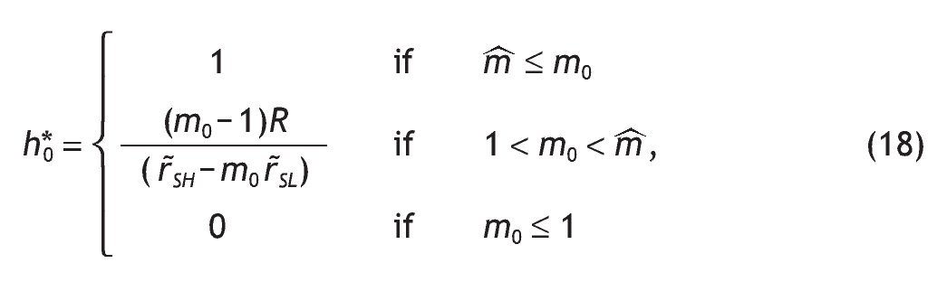
with
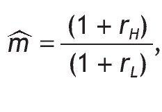
, and the corresponding m0 is
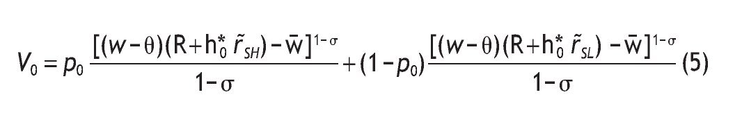
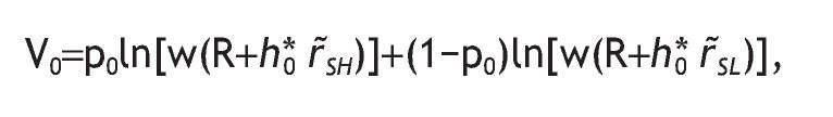
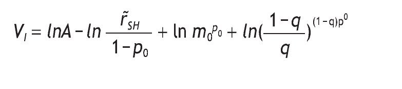
The indirect utility for uninformed investors is
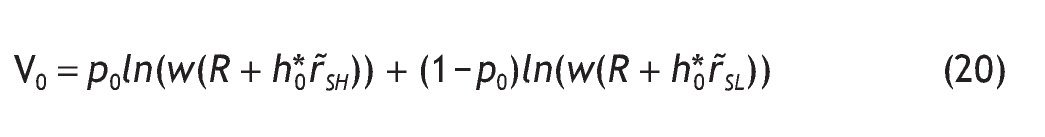
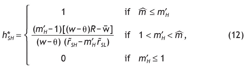
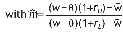
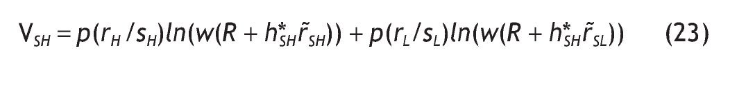
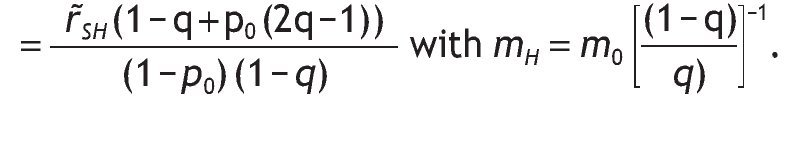
Next, to determine the indirect utility for informed agents, we do backwards induction. We first solve the decision problem for each possible signal received by the agent. We then use these contingent solutions to compute the expected utility prior to the observation of the signal. It is easy to show that when investors are endowed with a high signal, the optimal solution is
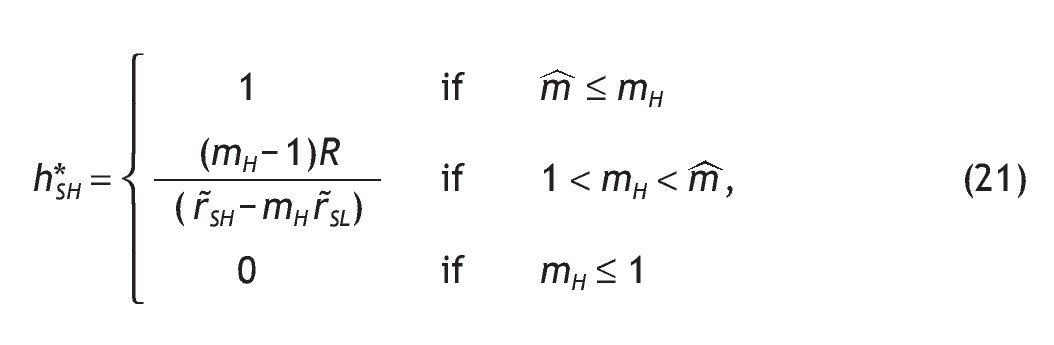
And the corresponding mH is
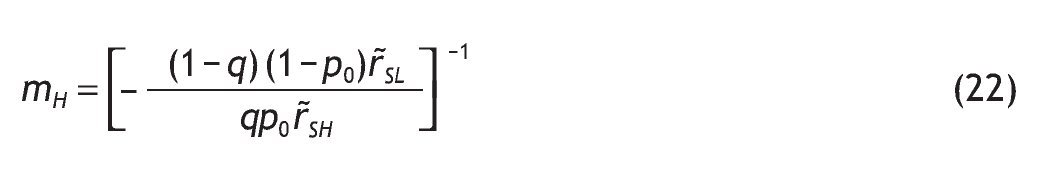
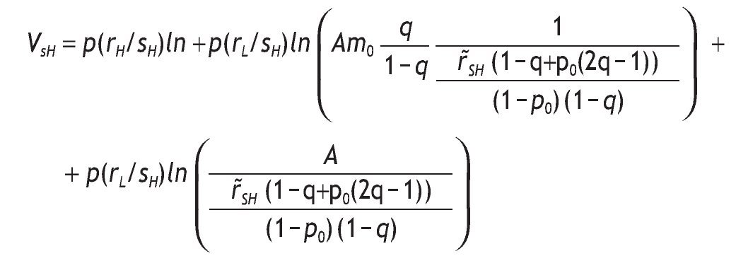
The indirect utility is
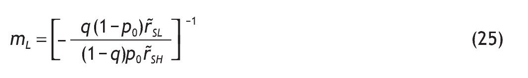
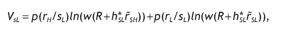
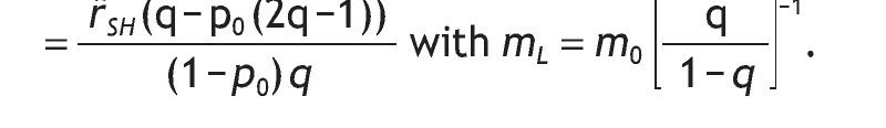
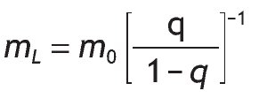
For agents receiving a low signal, the optimal investment in the risky asset is given by the following expression
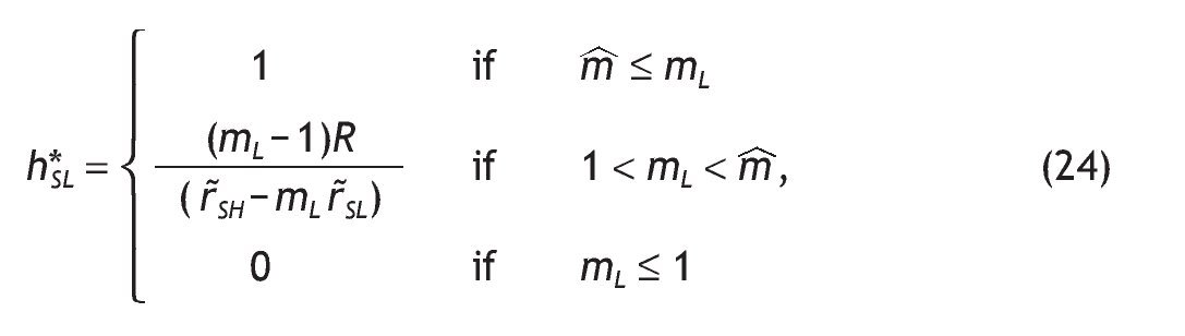
with mL given by
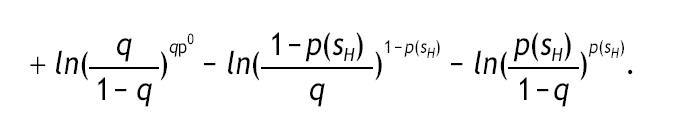
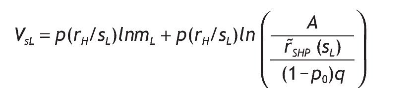
And the indirect utility function is
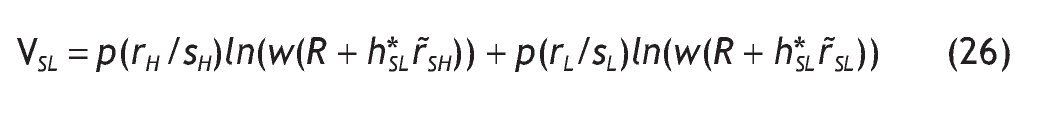
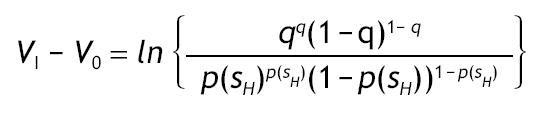
The value of information is given by the difference V I - V 0 = 0, with VI being the ex-ante utility of an informed agent, i.e. VI = p(sH)VSH + p(sL)VSL.13 In our model, by contrast, some agents would receive the private signal and some others would not. Therefore, the value of information is given by the difference V I - V 0. The next Proposition states which variables determine the value of information, and how they are related. As expected, the more accurate the information, the higher the value of having private information.
Proposition 3:
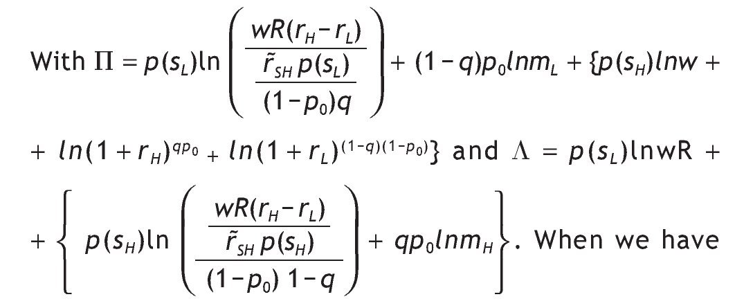
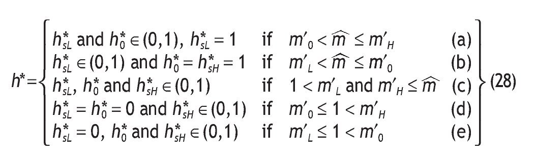
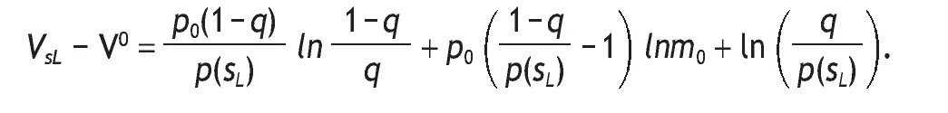
Under logarithmic preferences, and assuming w = θ = 0, A2 and p0>1/2, the value of acquiring private information is given by
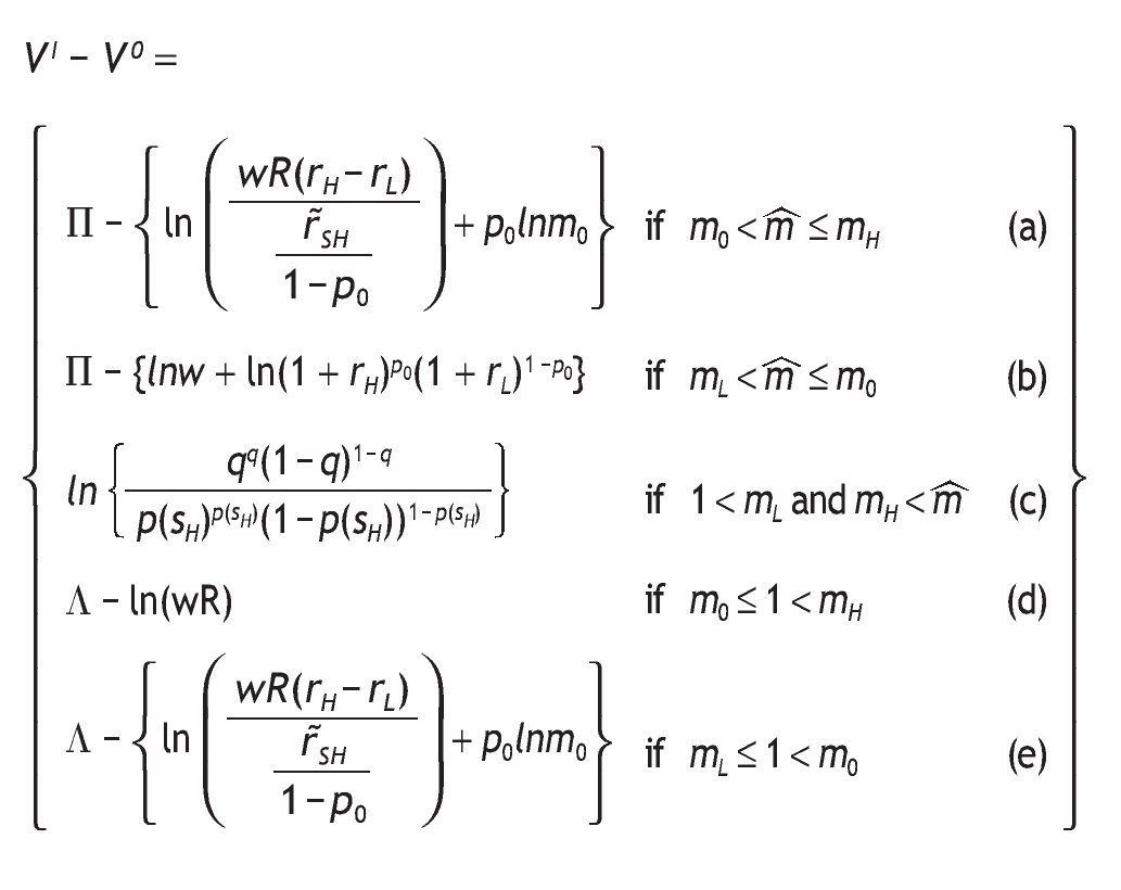
interior solutions, the value of information is increasing in the precision of the signal and decreasing in the initial prior.
Proof: See Appendix.
Proposition 3 distinguishes among five possible situations depending on the value of parameters, probabilities of events and returns. Intuitively, information is valuable only if portfolio choice becomes sensitive to the arrival of new information. This is not the case if we have corner solutions in all three scenarios, i.e. if receiving a high signal, if receiving a low signal, and without information, when the agent receives a high signal, a low signal or not information at all.14 In these cases, information is useless for the decision maker given that V I = V 0. In contrast, information is valuable only if observing private information would reverse the decision. This is so for case (c), that is, when different interior solutions are obtained,15 i.e. h*0, h*SL and h*SH Î (0,1) depending on the information received. In these circumstances, variables like wealth, the risk-free rate or the level of payoffs do not matter in explaining the value of information. Indeed, the value of information is affected by the precision of the signal, as well as the probability of having a good state. The proposition shows that the more precise the private information, the higher the value of that information. And the larger the initial prior of having a high return, the less useful that information.
Notice that under mL ≤ 1 < m0 having no information is similar to having a high signal because h*0 and h*SH Î(0,1) and under m0 ≤ 1 < mH receiving no information is similar to receiving a low signal since h*0 = h*SL = 0. Similarly, comparing mL < m ≤ m0 with m0 < m ≤ mH, in the first case h*0 = h*SH = 1, and under m0 < m ≤ mH, both h*0 and h*SH Î(0,1) are interior solutions. In cases (a) and (e), h*0 is interior, and thus portfolio choice may differ among informed and uninformed agents. Here, apart from q and p0 new variables matter to determine the value of information, in particular, the risk-free rate and the level of payoff. Unfortunately, we cannot say much about how the value of information depends on these variables, since the sign of the partial derivative is undetermined.16
To conclude, in the next Proposition, we present the ex-post value of information (i.e., after the signal is realized) assuming interior solutions in all three cases, i.e. whether the individual receives a high signal, a low signal, or no information at all. We study how it depends on the precision of the signal.
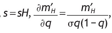
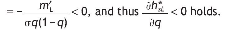
Proposition 4: Assume A1, w=θ=0, then conditional of having a high (low) signal, the value of information is increasing (decreasing) in its precision, that is
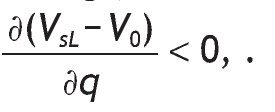
and
Proof: See Appendix.
Intuitively, the higher the precision, the more valuable is having a high signal. Whereas getting a very precise low signal reduces welfare compared to no receiving any signal at all.
5. Conclusions
We develop a partial equilibrium portfolio choice framework in which some agents receive a private signal on the return of the risky assets. These agents update their prior using Bayes' rule and portfolio decisions using the new prior. We compare this situation with the case of agents who simply have access to public information on the distribution of the risky return.
We find that the quality of information is a crucial variable in order to understand not only portfolio choice but also the value of information. First, asset allocation decisions among informed and uninformed investors differ only if the precision of the signal is high enough. We also show that investors endowed with a high accurate signal will invest more than uninformed agents and the larger the precision, the larger the amount invested in the risk asset.
Second, information is useful only if it is good enough. This is so because information is valuable only if portfolio choice becomes sensitive to the arrival of new information. This is the case under interior solutions with values differing on whether the signal is low, high or absent in all three cases, i.e. with a low signal, a high signal and without information. In this case, the value of information is affected by the precision of the signal, as well as the probability of having a good state, but it is not influenced by variables like wealth, risk-free rate and the level of payoffs. The paper shows that the more precise the signal, the higher the value of information; and the larger the initial prior of having a high return, the less useful is that information.
Our model is essentially static. However, it would be interesting to extend the model to a dynamic framework. This set up the challenge of will be difficult because one has to keeping track of the changes in the distribution of wealth (an object of infinite dimension) and solve for the hedging demands that they will induce. Under this framework, the next step in our research agenda is it will be interesting to understand how differences in information acquisition translate into differences in the accumulation of wealth.
Acknowledgements
Beatriz de Blas acknowledges financial support from ECO2008-04073 project of the Spanish MEC. Ana Hidalgo gratefully acknowledges the Spanish Ministry of Science and Innovation for their financial support through ECO2010-19596. The authors gratefully acknowledge the hospitality of the Economics Department at Columbia University and University of New York where part of this work was conducted.
Appendix
Proof of Lemma 1
A.
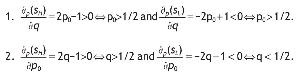
B.
If q>1/2 and p0>1/2 Þ p(sH) > p(sL) and if q<1/2 and p0<1/2 Þ p(sH) < p(sL). This is so because p(sH) > p(sL)Û q[2p0-1]>(1-q) [2p0-1].
C.
p(rH/sH) > p(rL/sH)Û qp>(1-q)(1-p0)Û p0>(1-q). Clearly, this inequality always holds under A1 and p0>1/2.
Proof of Proposition 1
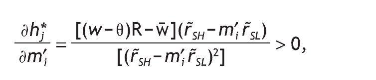
1. Notice that the two thresholds (i.e. 1 and m~) are independent on the signal received and that for any q>1/2, m′L < m′0 < m′H holds. Therefore, we could distinguish the following cases
Clearly,if m ≤ m′L (that is when h*sL = h*0 = h*sL = 1) and/or m′H ≤ 1 (that is when h*sL = h*0 = h*sL = 0), we have corner solutions in all three cases, i.e. with a high signal, with a low signal and without private information. On the contrary, when 1 < m′L and m′H ≤ m , all three solutions are interior and then h*sL < h*0 < h*sH holds since for any q>1/2, m′L < m′0 < m′H holds too. To analyze how h*j is affected by the precision we compute
for i={H,L} and j={SH,SL}. Conditional on receiving a high signal,
, so that
, and similarly, conditional on receiving a low signal,
2. For q=1 we have that p(rH/sH) = p(rL/sL) = 1. Consequently, the FOC under a high signal becomes
andthus, h*sH = 1 and the FOC under a low signal becomes [(w - θ)[R + hr˜SL] - w¿]- s (w - θ)r˜SL < 0 and thus h*sL = 0.
3. For q=1/2, m′L = m′0 = m′H holds too and thus, h*sL = h*0 = h*sH holds.
Proof of Proposition 2
The ex-ante average proportion invested in the risky asset is given by EI = h*sHp(sH) + h*sL p(sL). Clearly, corner solutions are independent on q, so we concentrate on interior solutions. If we substitute the optimal interior solutions of h*sH and h*sL we obtain
Define
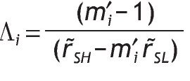
for i={H,L}, with its partial derivative given by
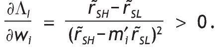
. Similarly,
By using Lemma 1.A., we know that
Ûp0>1/2, therefore
with Σ=[(w-θ)R-w]/(w-θ). Under A1, this derivative is positive since m′H - m′L > 0, and by using Lemma 1.B p(sH) > p(sL) always holds.
The average volume of investment in the risky asset with a high signal is increasing with q, that is
the derivative is positive because
and by
Lemma 1.A
The average volume of investment in the risky asset with a low signal is decreasing with q, that is
the derivative is negative because
by Lemma 1.A
Proof of Proposition 3
Equation (27) comes from equation (28) above. Let's concentrate on the case of 1 < mL and mH < m~ that is when we have interior solutions. First, we solve the indirect utility function for non-informed and informed agents when the solutions are interiors. And then, we compute the ex-ante indirect utility of an informed agent.
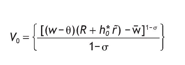
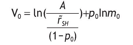
Indirect utility of the non¿informed agents:
Under the logarithmic utility function, and assuming thatθ=w=0, the indirect utility of the non-informed agents is given by:
substituting the value of h*0 and m0, we obtain
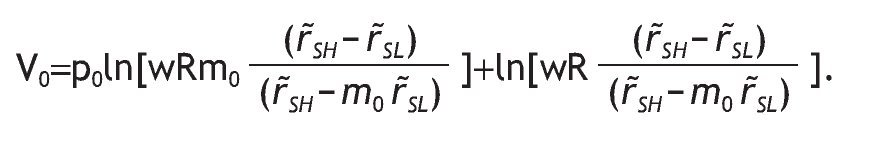
Let's define A=wR (r˜SH - r˜SL). The value of r˜SH - m0 r˜SL can be rewritten as r˜SH - m0 r˜SL = r˜SH/(1-p0), with
Thus, the indirect utility becomes
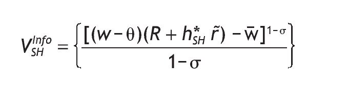
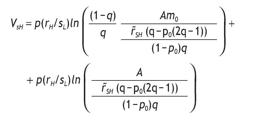
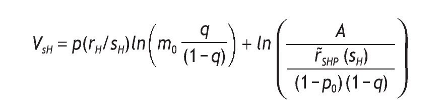
Indirect utility of the informed agents conditional of having a high signal:
The indirect utility of the informed agents when the signal is high is
substituting the value of h*SH and mH, we obtain
after some calculations, we find that r˜SH - mHr˜SL =
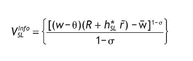
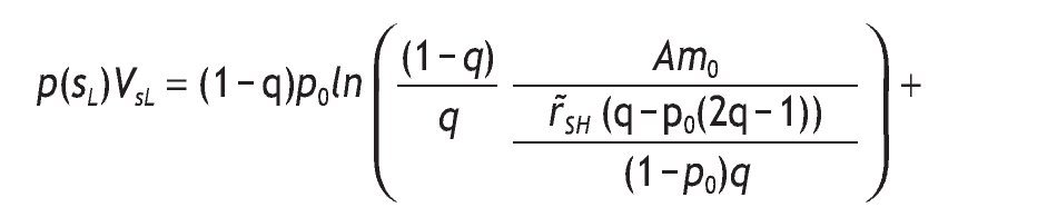
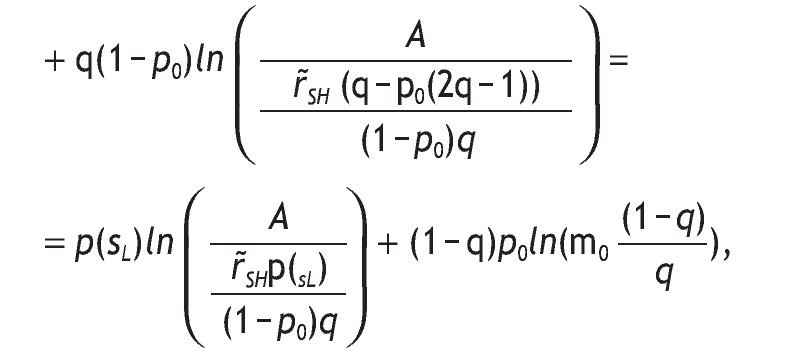
Indirect utility of the informed agents conditional of having a low signal:
The indirect utility of the informed agents when the signal is low is
after some calculations, we find that r˜SH - mHr˜SL =
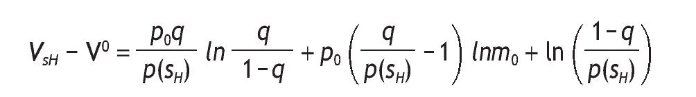
The ex¿ante indirect utility of an informed agent:
Before the signal is received, informed agents have the following indirect utility
VI = p(sH)VsH + p(sL)VsL.
Taking into account VsH and VsL and the fact that p(sH)p(rH/sH) = = qp0,p(sH)p(rL/sH) = (1 - q)(1 - p0) and similarly, p(sL)p(rH/sL) = = (1 - q)p0,p(sL)p(rL/sL) = q(1 - p0), we can rewrite p(sH)VsH as
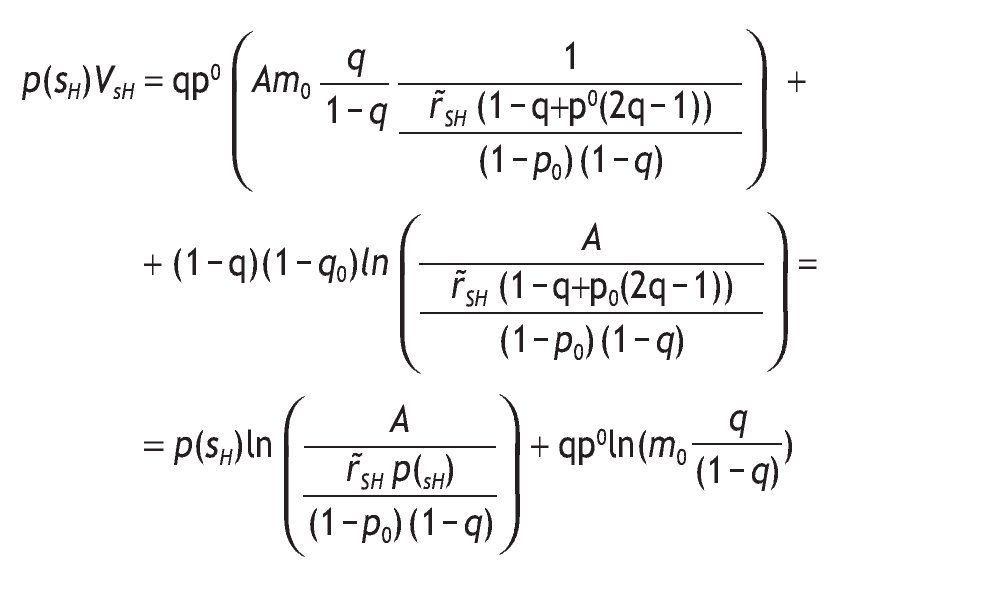
and we can rewrite p(sL)VsL as
and thus,
where 1 - p(sH) = q - p0(2q - 1) and p(sH) = (1 - q) + p0(2q - 1). Therefore, the value of information is given by
Let's define VI - V0 = Ψ,
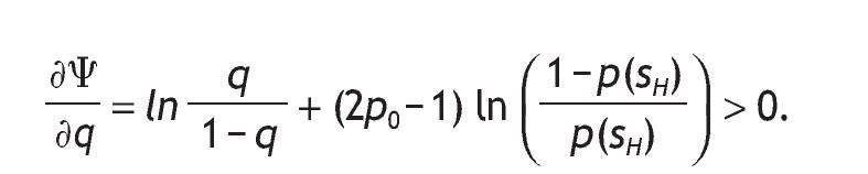
We know that under,
< 1, with
Moreover, 1>2p0-1 holds. And thus, the sign of this derivative is positive.
The value of having private information decreases with p0,
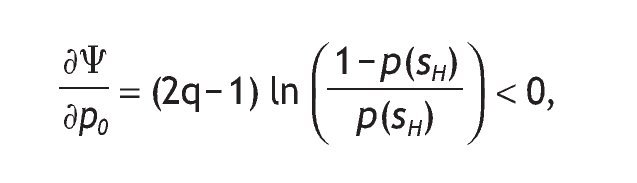
because if A1 and p0>1/2 holds, then p(sH) > 1 - p(sH) holds too.
Proof of Proposition 4
First, we need to compute the indirect utility of informed versus uninformed agents, and then we will compute the difference. We concentrate in the case of interior solutions.
From proposition 3, we have computed the indirect utility on informed agents with a high signal as
And the Indirect utility of the non-informed agents, V0
By computing VsH - V0: the difference is giving by
Notice that if q=(1/2), then ln
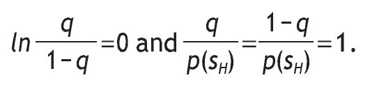
Therefore, VsH = V0.
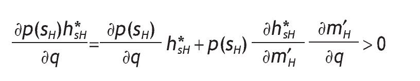
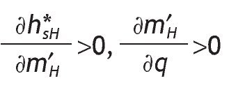
Finally, if p0 > (1/2), then VsH - V0 is increasing with q. That is
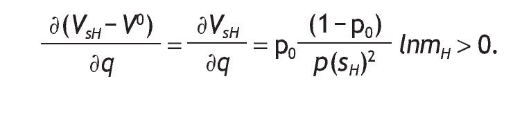
From proving proposition 3, we have computed the indirect utility on informed agents with a low signal as
using mL = m0
we compute the difference
Notice that if q=(1/2), then
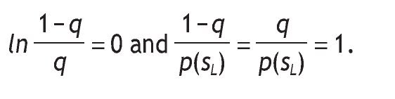
Therefore, VsL = V0-
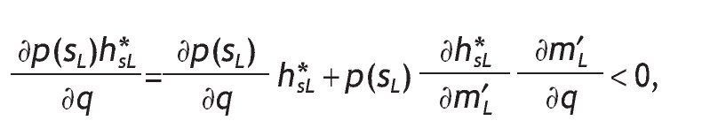
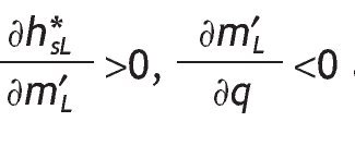
Finally, if A1 holds, the equation VsL - V0 is decreasing with q, this is so because
1. There is wide evidence that information affects not only the expected return of the risky asset, but also market prices (see for example Tetlock et al., 2008). However, we abstract from this second effect since asset pricing is beyond the scope of this paper.
2. For an analysis of the welfare cost of non-participation in the stock market as well as the efficiency of household investment decisions using Swedish panel data, see Calvet et al. (2007).
3. Wachter and Yogo (2010) show that the non-homothetic life- cycle model quantitatively explains the empirical fact that portfolio share rises in wealth.
4. As we will mention later on, there is strong evidence supporting the presence of participation costs (Vissing-Jorgensen, 2002; Poterba & Samwick, 1997).
5. Clearly, this definition is arbitrary, and when qÎ (0,1/2) the signal s = sL should be called the good signal, and the correlation between the signal and the return is negative. Indeed, when q is 0, there is a perfect negative correlation and the information is perfect.
6. Clearly, it is not the case in corner solutions, that is, when h*SL = h*0 = h*SH = 1 and/or h*SL = h*0 = h*SH = 0. Similarly, as detailed in the appendix, if m'L < m < m0, then h*SL Î (0,1) and h*0 = h*SH = 1. And, if m0 < 1 < m'H, then h*0 = h*Sl = 0 and h*SH Î (0,1).
7. Home bias occurs when investors seem to over-weight their home country assets in their equity portfolios.
8. For studies that incorporate the effect of information's contents on asset prices, see for example Tetlock et al. (2008) who empirically analyzes information's content, using linguistic methods to measure the extent to which each new item is positive or negative. Specifically, Tetlock et al. (2008) examine all Wall Street Journal and Dow Jones News Service articles about individual S&P 500 firms from 1980-2004. They count the number of negative words in each article and show that this verbal information is incorporated into market prices for the firm's equity on the subsequent day.
9. With corner solutions, the expression EI becomes trivial for analyzing comparative statics.
10. For this example, we set θ = w = 0, rH = 15%, rF = 10%, rL = 3%, p = 0.6, and q = 0.6.
11. This is so because more information before acting would reduce risk.
12. For any θ,w > 0, the results do not change qualitatively.
13. If the entrance decision were endogenous, in equilibrium, agents would decide to acquire information until V I - V 0 = 0.
14. Specifically, we have that h*0 = h*sH = h*sL = 1 if m ≤ mL and h*0 = h*sH = h*sL = 0 if mL ≤ 1.
15. Clearly, when we assume 1 < mL and mH < m .
16. We just could be sure that under m0 < m ≤ mH the value of information is increasing with (1 + rH) and with (1 + rF), and it is independent on wealth under m0 < m ≤ mH and mL ≤ 1 < m0.
Received February 8, 2012; accepted March 27, 2012
*Corresponding author.
E-mail address: beatriz.deblas@uam.es (B. de Blas).
References
Alessie, R.S., Hochguertel I.S., Van Shoest, A., 2002. Households portfolios in the Netherlands. In: Guiso, L., Haliassos, M., Jappelli, T. (Eds.), Household portofolios. MIT Press, Cambridge, MA.
Bertola, G., Foellmi, R., Zweimüller, J., 2006. Income distribution in macroeconomic models. Princeton University Press, Princenton, NJ.
Bonaparte, Y., 2006. Why do wealthy investors have a higher return on their stocks? Mimeo, The University of Texas at Austin.
Borsch-Supan, A., Eymann, A., 2002. Household portfolios in the United States. In: Guiso, L., Haliasos, M., Jappelli, T. (Eds.), Household Porfolios. MIT Press, Cambridge, MA.
Calvet, L., Campbell, J., Sodini, P., 2007. Down or out: Assessing the welfare costs of household investment mistakes. Journal of Political Economy 115, 707-747.
Eeckhoudt, L., Gollier, C., Schlesinger, H., 2005. Economic and financial decisions under risk. Princeton University Press, Princenton, NJ.
Grossman, S., Stiglitz, J., 1980. On the impossibility of informationally efficient markets. American Economic Review 70 (3), 393-408.
Guiso, L., Jappelli, T., 2002. Household portofolios in Italy. In: Guisi, L., Haliassos, M., Jappelli, T. (Eds.), Household portfolios. MIT Press, Cambridge, MA.
Hong, H., Kubik, J.D., Stein, J.C., 2004. Social interaction and stock-market participation. Journal of Finance 59 (1), 137-163.
King, M., Leape, J., 1987. Asset accumulation, information and the life cycle. NBER Working Paper 2392.
Mankiw, N.G., Zeldes, S.P., 1991. The consumption of stockholders and nonstockholders. Journal of Financial Economics 29 (1), 97-112.
Peress, J., 2004. Wealth, Information Acquisition, and Portfolio Choice. Review of Financial Studies 17 (3), 879-914.
Persico, N., 2000. Information Acquisition in Auctions. Econometrica 68 (1), 135-148.
Poterba, J.M., Samwick, A., 1997. Household portfolio allocation over the life cycle. NBER Working Paper, 6185.
Tetlock, P., Saar-Tsechansky, M., Macskassy, S., 2008. More than words: Quantifying language to measure firms' fundamentals. Journal of Finance 63 (3), 1437-1467.
Treich, N., 1997. Risk tolerance and value of information in the standard portfolio model. Economics Letters 55 (3), 361-363.
Van Nieuwerburgh, S., Veldkamp, L., 2009. Information immobility and the home bias puzzle. Journal of Finance 64 (3), 1187-1215.
Veldkamp, L., 2011. Information choice in macroeconomics and finance. Princeton University Press, Princeton, NJ.
Vissing-Jorgensen, A., 2002. Towards an explanation of household portfolio choice heterogeneity: Nonfinancial income and participation cost structures. NBER Working Paper, 8884.
Vissing¿Jorgensen, A., 2004. Perspectives on behavioral finance: Does 'irrationality' disappear with wealth? Evidence from expectations and actions. NBER Macroeconomics Annual 2003, 139-208.
Wachter, J., Yogo, M., 2010. Why do households portfolio shares rise in weath forthcoming. Review of Financial Studies 23, 3929-3965.