Multivariate exploratory data analysis for large databases: An application to modelling firms’ innovation using CIS data

Abstract

This paper argues that, when using a large database, organizational researchers would benefit from the use of specific multivariate exploratory data analysis (MEDA) before performing statistical modelling. Issues such as the representativeness of the database across domains (countries or sectors), assessment of confounding among categorical covariates, missing data, dimension reduction to produce performance indicators and/or remedy multicollinearity problems are addressed by specific MEDA. The proposed MEDA is applied to data from the Community Innovation Survey (CIS), a large database commonly used to analyse firms’ innovation activities, prior to fitting ordered logit and Tobit regression models. A set of recommended practices involving MEDA are proposed throughout the paper.

Introduction

Over the last decades, the volume of data gathered and stored has reached unprecedented levels. In business, the collection of such large amounts of data compels managers and researchers to develop new approaches to exploit and best address the information contained in what are usually large and complex databases. To understand the potential and limitations of statistical content in such databases, the present paper argues that researchers would benefit from using multivariate exploratory data analysis that are currently available in statistical software packages – both proprietary software, such as SPSS or Stata, and free software, such as R. When large databases are involved, we advocate the use of MEDA before estimating and testing complex theoretical-based models. Such ‘pre-modelling’ statistical analysis encompasses the display of clusters, heterogeneity and confounding of variables, data transformation, the presence of missing data, dimension reduction and ‘index construction’, among other tools.

The paper uses the Community Innovation Survey (CIS) (Eurostat, 2008) to illustrate how specific MEDA can be applied with large databases in organizational research. This database of European firms collects information on different types of firm innovation outcomes (product, process, organizational and marketing innovations) as well as a wide range of indicators of activities that are understood to promote firm innovation. The CIS database has been extensively used in research aiming to relate the impact of firms’ innovation activities with their actual innovation performance (e.g., Cassiman and Veugelers, 2002; Laursen and Salter, 2006; Frenz and Ietto-Gillies, 2009; Hashi and Stojčić, 2013, and others).

The MEDA practices we describe are not new in the statistical literature and aim to follow the spirit of exploratory data analysis (Tukey, 1977; Cook and Weisberg, 1994; Kirk, 2012). In our view, however, MEDA is not sufficiently used in the practice of organizational research. This paper discusses a set of recommended practices (hereafter RPs) that give a step-by-step guidance to MEDA when modelling in a large database. These RPs are then illustrated by fitting ordered logistic and Tobit regression models to CIS data.

Although many MEDA methods may be considered, the present paper focuses on those that we feel are of general use in organizational research. The methods considered address the following issues:

• 1.

  Sample size representativeness across multiple domains, e.g. across countries and sectors, with the aim of uncovering the (over/under) representativeness of the database in domains of interest.

• 2.

  Missing data analysis. Description (and visualization) of the severity of missing data across cases and variables, identifying patterns of missing data and their potential impact on the analysis, and modern approaches to missing data under different assumptions about the mechanism leading to missingness.

• 3.

  Dimension reduction in both covariates and the dependent variables. When a large dataset is involved, it is often necessary to avoid multicollinearity problems and the loss of degrees of freedom due to partial redundancy of explanatory variables. The dependent variable by itself may involve several indicators (for example, in our database, the different types of innovation) that can lead to a single index of innovation performance.

The MEDA methods described in the paper can be performed using the current software in use in organizational research, such as Stata, SPSS and R. For completeness, Appendix 3 contains the code in R (R Core Team, 2016) of all the statistics of the paper.

The paper is structured as follows. Section “The Community Innovation Survey” describes the CIS database and the scope, variables and structure of the survey. Section “Sampling representativeness of countries and sectors” explores the sample representativeness of the CIS across its key domains, countries and sectors. Section “Missing data” describes the patterns for missing data across variables and domains and discusses various approaches to the problem of missing data. Section “Dimension reduction” deals with issues of data dimension reduction in both the dependent variables and covariates. Section “Modelling innovation: an illustration” presents the actual modelling of innovation performance using ordered logistic and Tobit regressions. The paper ends with a discussion.

The Community Innovation Survey

The CIS is a European database that has been widely used in firm innovation studies (Cassiman and Veugelers, 2002; Laursen and Salter, 2006; Frenz and Ietto-Gillies, 2009; Hashi and Stojčić, 2013). It is a sampling-based database that targets the population of firms with more than 10 employees, located in European countries, and operating in the manufacture and service sectors. The data are collected every two years through a harmonized survey questionnaire delivered by the European Union (EU) member states.¹ The data are gathered through a combination of postal and electronic surveys addressed to the heads of R&D or innovation departments. Within each country, the firms are classified into 24 sectors using the Statistical classification of economic activities in the European Community (NACE), revision 2, at the 2-digit level. The list of sectors is provided in Appendix 1. For the sample collection within each country, the sector and the size of the firm (number of employees) are used as stratifying factors.²

This paper uses the CIS 2008, variables referring to the period of 2006–2008. The firms are classified by two main domains: country and sector. Although the CIS 2008 survey compiled information from all the 27 countries that were members of the EU in 2006 and Norway, confidentiality issues and agreements between Eurostat and EU members limited our database to the following 16 countries: Bulgaria (BG), Cyprus (CY), Czech Republic (CZ), Germany (DE), Estonia (EE), Spain (ES), Hungary (HU), Ireland (IE), Italy (IT), Lithuania (LT), Latvia (LV), Norway (NO), Portugal (PT), Romania (RO), Slovenia (SL), and Slovakia (SK). A total of n = 127,674 firms, unevenly distributed across 16 countries and 24 sectors are included in the analysis.

Our CIS 2008 database has 181 variables; some are related to firms’ innovation performance (used as dependent variables in the analysis), whereas others are indicators of firms’ innovation promoting activities (termed covariates).³ Regarding the dependent variables, the CIS follows the Oslo Manual (OECD, 2005), and considers four types of innovations: (a) product innovations, inprod (new or significantly improved goods or services); (b) process innovations, inproc (new or significantly improved production processes, distribution methods, or support activities); (c) organizational innovations, inorg (new organizational methods, workplace organization or external relations); and (d) marketing innovations, inmkt (implementation of a new marketing concept or strategy, including changes in product design, packaging, product placement, product promotion or pricing). The variables inprod, inproc, inorg and inmkt are binary variables classifying the firms as ‘innovator’ or ‘non-innovator’ in terms of the different type of innovations.⁴ Note that the types of innovation are not mutually exclusive, and firms can be classified as ‘innovators’ in terms of more than one type of innovation.

The CIS also includes variables measuring the intensity of the product innovation: the variables turnmar (percentage of total turnover from product innovations that are new to the market) and turnin (percentage of total turnover from product innovations that are only new to the firm). Turnmar and turnin have been considered as measures of radical and incremental innovation, respectively (e.g., Laursen and Salter, 2006; Van Beers and Zand, 2014; Doran and Ryan, 2014).⁵

In turn, we distinguish two types of covariates: demographic covariates, designed to be observed for all the firms, and innovation-related variables, which are only available for firms that have engaged in (aiming to promote) some type of firm innovation.

Demographic covariates include general information about the firm (see sections 1 and 11 of the questionnaire). These variables are: the country of origin of the head office of the firm (country); the industry in which the firm operates (nnace), using a sectoral classification based on NACE; whether the firm and the head office are in the same country (ho); whether the firm is independent or part of a group (gp); the geographic markets in which the firm sells its products, classified as local/regional (marloc), national (marnat), other EU countries (mareur), or all other countries (maroth); the geographic area of the largest market in terms of turnover (larmar); and a measure related to the size of the firm: turnover in 2006 (turn06). Note that except for turn06 and larmar, all these variables are binary. See Appendix 2 for a description of the set of variables in the CIS and how they are measured.

For firms engaged in product or process innovations (i.e., inproc = 1 or improd = 1, the questionnaire contains a large set of innovation-related variables (see sections 5 and 6 of the questionnaire). These variables are: (1) innovation activities such as in-house R&D, external R&D or acquisition of machinery (8 variables); (2) innovation expenditures, including in-house R&D and purchase of external R&D (5 variables); (3) innovation objectives such as an increased range of goods or services, entry in new markets, and increased market share (9 variables); (4) sources of information, including suppliers, clients or customers, and universities, among others (10 variables); (5) cooperation with partners (9 variables); and (6) public funding for innovation activities (4 variables).⁶ Since our applications focus on product innovation, other innovation-related covariates associated with organizational and marketing innovation, or innovations with environmental benefits (a total of 29 variables) are not included in the analysis.

To summarize, the CIS reports information on a large set of variables for a random sample of firms extracted from different population domains, such as countries and sectors. One key aspect of this database is that it is sampling-based. The variation of the sample size across domains is an issue that must be examined before any statistical modelling is performed.

Following this description of the database, we now introduce specific MEDA methods that can assist in modelling.

Sampling representativeness of countries and sectors

Statistical modelling aims to find relations that apply to units that may belong to different domains, e.g., the case of firms from different countries or sectors. A proper balance of sample size across the different domains must be monitored (i.e., to avoid over- or under-representation of firms from a specific country or sector) to decide whether weighting is necessary when pooling units across domains. Sample size representation across domains must therefore be examined.

The two categorical variables (factors) that define key domains in our study are the country and sector of the firm. An initial question to address here is sample representativeness, that is, assessing whether the representation of firms in each of these domain categories is appropriate. These two variables can also be regarded as potentially explanatory factors for firms’ innovation, in line with the commonly held view that certain countries (or sectors) may perform differently in terms of innovation. The second question concerns the possibility of confounding between the two domains, that is, whether some countries are over- or under-represented in certain sectors. This leads to the MEDA methods we describe in the following subsections.

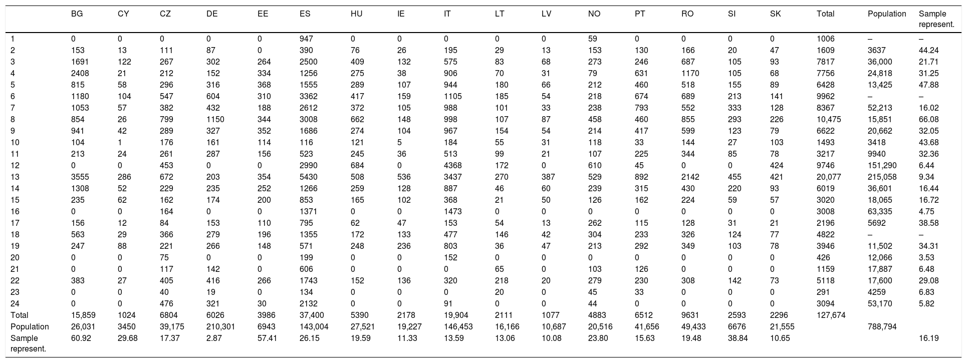
Sampling representativeness

Table 1 presents the contingency table obtained by cross-classifying firms in terms of country (country) and sector (nnace). The marginal rows and columns ‘Total’ give the CIS sample size of the different countries and sectors, respectively. For the marginal cells, both for countries and sectors, population size is available from an external source, in our case the total number of active firms in the European Union.⁷ The initial contingency table has, thus, been expanded with: (1) the marginal rows and columns ‘Population’, which gives the population size of each category of the domain; and (2) the marginal row and column ‘Sample representativeness’, which shows the ratio between the CIS sample size and the population of active firms.⁸ For the sake of simplicity, we have confined the representativeness of the sample to the marginal for country and sector. Comparison could have been made for each cell of the contingency table, in which case a substantive discrepancy between sample and population would suggest weighting for country and sector jointly.

Table 1.

Contingency table of number of firms in the CIS database: cross-classified by country and sector (sample representativeness of the database is informed by additional rows and columns).

	BG	CY	CZ	DE	EE	ES	HU	IE	IT	LT	LV	NO	PT	RO	SI	SK	Total	Population	Sample represent.
1	0	0	0	0	0	947	0	0	0	0	0	59	0	0	0	0	1006	–	–
2	153	13	111	87	0	390	76	26	195	29	13	153	130	166	20	47	1609	3637	44.24
3	1691	122	267	302	264	2500	409	132	575	83	68	273	246	687	105	93	7817	36,000	21.71
4	2408	21	212	152	334	1256	275	38	906	70	31	79	631	1170	105	68	7756	24,818	31.25
5	815	58	296	316	368	1555	289	107	944	180	66	212	460	518	155	89	6428	13,425	47.88
6	1180	104	547	604	310	3362	417	159	1105	185	54	218	674	689	213	141	9962	–	–
7	1053	57	382	432	188	2612	372	105	988	101	33	238	793	552	333	128	8367	52,213	16.02
8	854	26	799	1150	344	3008	662	148	998	107	87	458	460	855	293	226	10,475	15,851	66.08
9	941	42	289	327	352	1686	274	104	967	154	54	214	417	599	123	79	6622	20,662	32.05
10	104	1	176	161	114	116	121	5	184	55	31	118	33	144	27	103	1493	3418	43.68
11	213	24	261	287	156	523	245	36	513	99	21	107	225	344	85	78	3217	9940	32.36
12	0	0	453	0	0	2990	684	0	4368	172	0	610	45	0	0	424	9746	151,290	6.44
13	3555	286	672	203	354	5430	508	536	3437	270	387	529	892	2142	455	421	20,077	215,058	9.34
14	1308	52	229	235	252	1266	259	128	887	46	60	239	315	430	220	93	6019	36,601	16.44
15	235	62	162	174	200	853	165	102	368	21	50	126	162	224	59	57	3020	18,065	16.72
16	0	0	164	0	0	1371	0	0	1473	0	0	0	0	0	0	0	3008	63,335	4.75
17	156	12	84	153	110	795	62	47	153	54	13	262	115	128	31	21	2196	5692	38.58
18	563	29	366	279	196	1355	172	133	477	146	42	304	233	326	124	77	4822	–	–
19	247	88	221	266	148	571	248	236	803	36	47	213	292	349	103	78	3946	11,502	34.31
20	0	0	75	0	0	199	0	0	152	0	0	0	0	0	0	0	426	12,066	3.53
21	0	0	117	142	0	606	0	0	0	65	0	103	126	0	0	0	1159	17,887	6.48
22	383	27	405	416	266	1743	152	136	320	218	20	279	230	308	142	73	5118	17,600	29.08
23	0	0	40	19	0	134	0	0	0	20	0	45	33	0	0	0	291	4259	6.83
24	0	0	476	321	30	2132	0	0	91	0	0	44	0	0	0	0	3094	53,170	5.82
Total	15,859	1024	6804	6026	3986	37,400	5390	2178	19,904	2111	1077	4883	6512	9631	2593	2296	127,674
Population	26,031	3450	39,175	210,301	6943	143,004	27,521	19,227	146,453	16,166	10,687	20,516	41,656	49,433	6676	21,555		788,794
Sample represent.	60.92	29.68	17.37	2.87	57.41	26.15	19.59	11.33	13.59	13.06	10.08	23.80	15.63	19.48	38.84	10.65			16.19

Measures of independence: χ² = 38,050, df = 345 (p-value < 0.001).

Contingency coefficient = 0.476.

Note: Information in these cells is not reported by Eurostat. This also causes missing information in the corresponding cell in the row and columns ‘Sample representativeness’.

The row ‘Total’ by countries shows clear and notable differences in sample size across countries and sectors. For instance, Spain (37,400 firms) and Italy (19,904) have much larger samples than, for instance, Germany (6026 firms). A simple way to assess whether the sample size of each country equally represents the population of firms in the country is to examine the ‘sample representativeness’ (last row and column in Table 1). Numbers different from 16.19 (the average representativeness in the whole sample) indicate an imbalance of the database in a given category (country or section). Inspection of these figures clearly shows that some countries are under-represented (values below 16.19) while others are over-represented (values above 16.19) in the database.

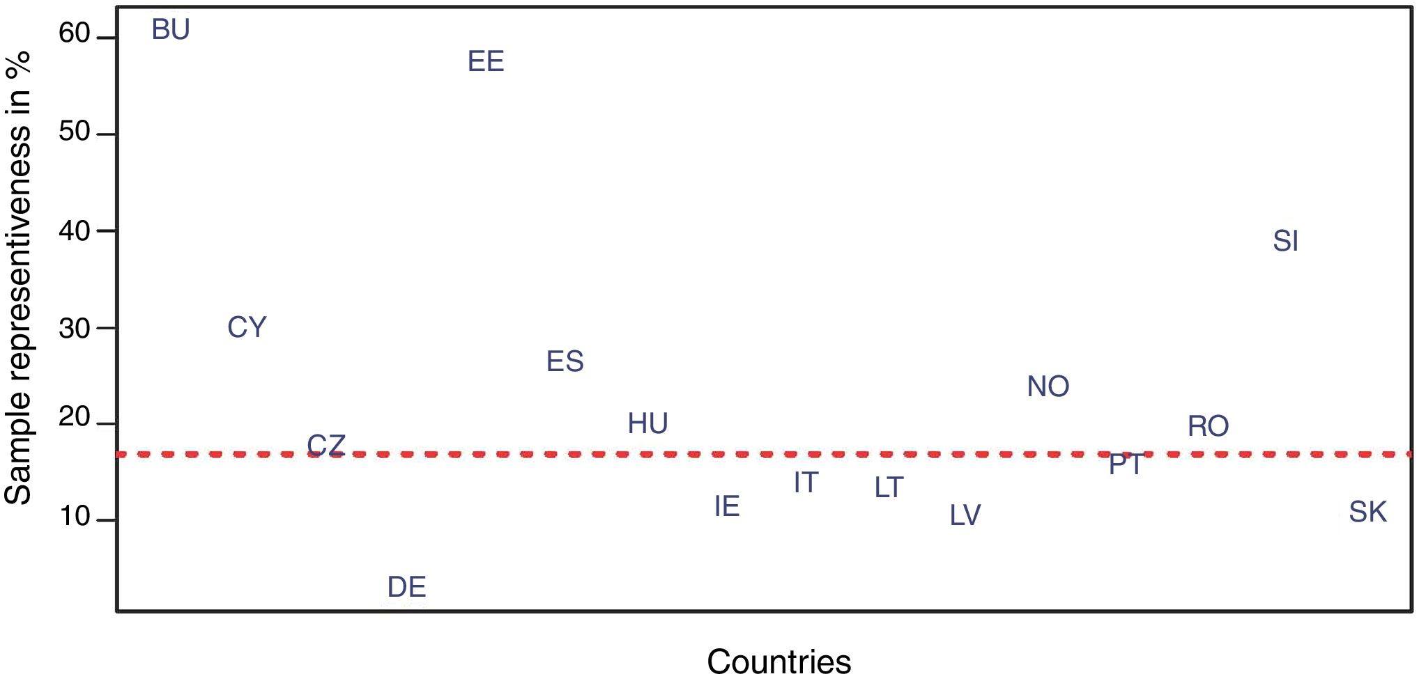
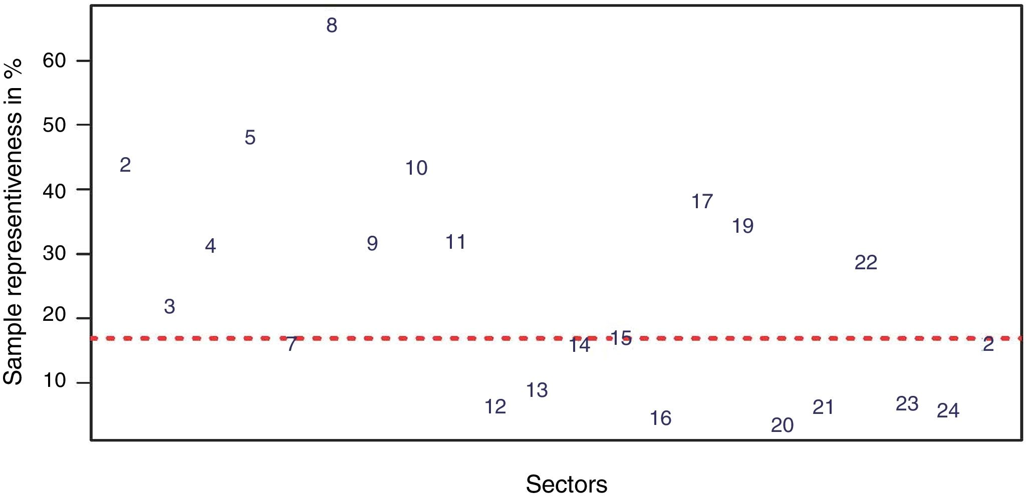
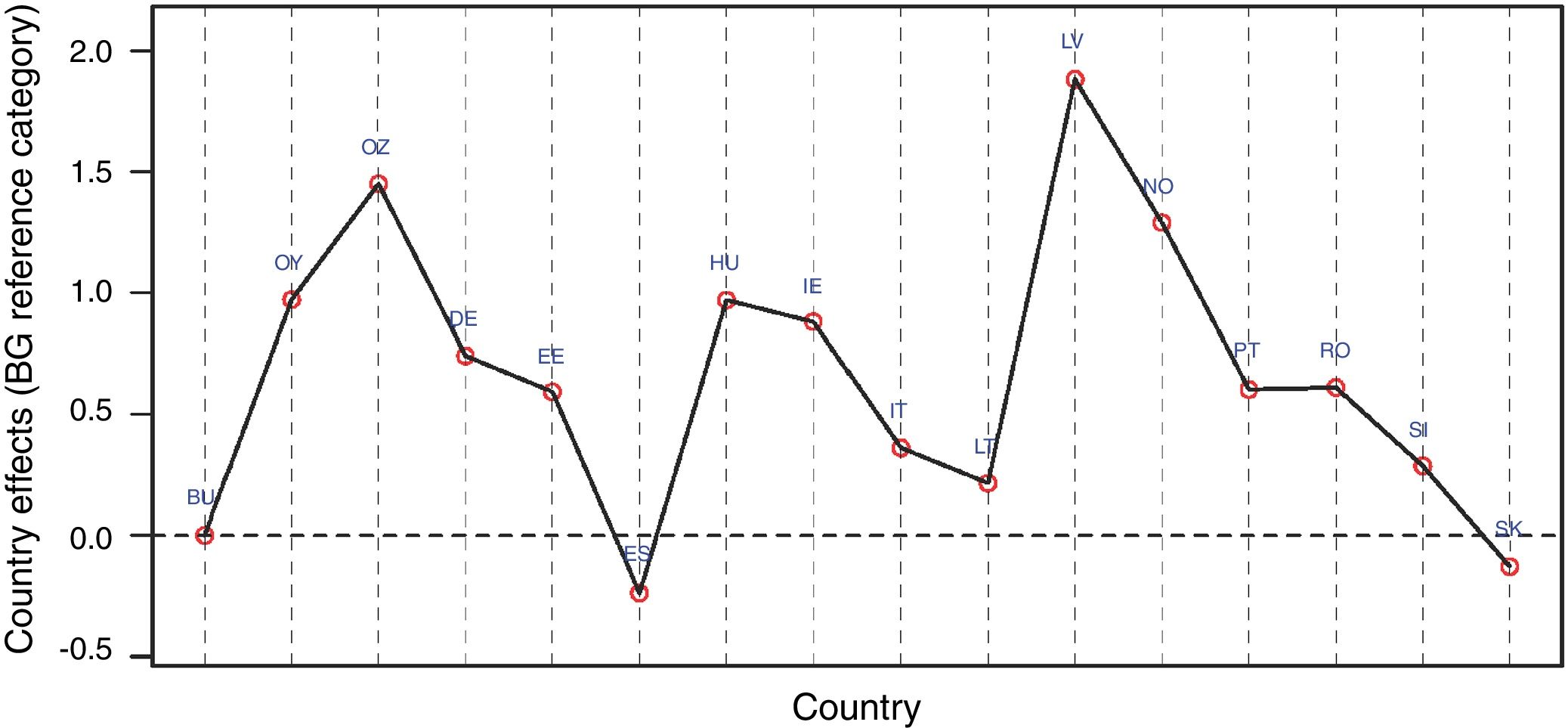
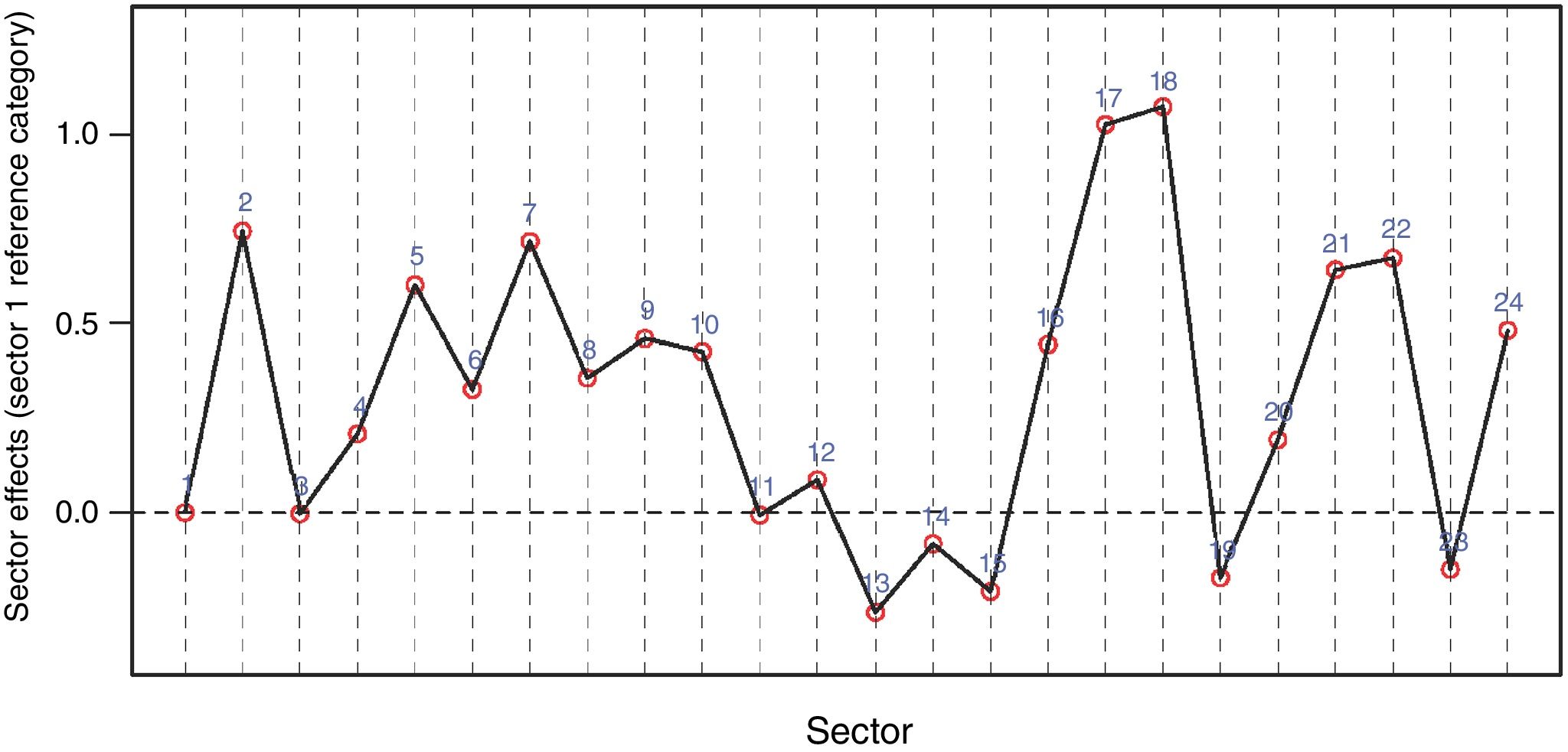
A simple visual display of sample size representativeness for countries and sectors is shown in Figs. 1 and 2. The horizontal red line in the scatterplots depicts the average sample representativeness for the whole sample. Fig. 1 reveals, for example, that Bulgaria and Estonia, well above the horizontal red line, are over-represented in the sample, while other countries such as Germany and Latvia fall below the reference line, and are thus under-represented. Similarly, Fig. 2 shows that, for example, sectors 9 (Manufacture of furniture; Repair of machinery and equipment) and 5 (Manufacture of wood; paper; printing) are over-represented in the sample.

Figure 1.

Sample representativeness across countries.

Figure 2.

Sample representativeness across sectors.

Imbalance of sample size representation across countries means that in addition to the weighting within each country, when the data is pooled across countries, a further weighting adjustment for countries must be made (see, for example, Srholec and Verspagen, 2012). The same reasoning applies to those studies analysing (one or multiple) sectors by pooling data from different countries. Obviously, since imbalance may distort the statistical analysis, pooling firms across countries without weighting would not be appropriate. One option for the analysis, when appropriate weights for the pooled data are lacking, would be multiple group analysis (see, for example, Rangus et al., 2016; Robin and Schubert, 2013), in which the groups are defined by the second-level units (countries or sectors), or a combination of them. Therefore, the potential for imbalance leads to the following recommended practice (RP1):

• •

  Recommended practice 1 (RP1): Assess possible imbalance of sample size representation for different domains defined by one or more categorical variable, in our example, countries and sectors. This assessment can be performed using a contingency table, such as Table 1. When population data is available for some of the cells, comparison of population and actual sample size is useful, as in Figs. 1 and 2. Disproportionate representation for some cells should prevent pooling units across domains without appropriate weighting.

The categorical variables for countries (country) and sector (nnace) can also be viewed as potential explanatory variables for innovation. In this case, confounding is an issue. We assess the potential confounding among countries and sectors using correspondence analysis.

Confounding

In the case of two categorical variables, confounding (i.e., the effect of the two variables cannot be disentangled) is associated with the existence of association (or lack of independence) among rows and columns in a contingency table (similar to the case of continuous covariates, where confounding is associated with high correlation). In our example of countries and sectors, an interesting table to explore the possible existence of confounding is that representing the sector profile for each country, i.e., for a specific country, the proportion of firms in each sector. High dissimilarity among these profiles would indicate variations in countries’ sectoral specializations, and would be an indication of confounding (the sector effect cannot be disentangled from the country effect).

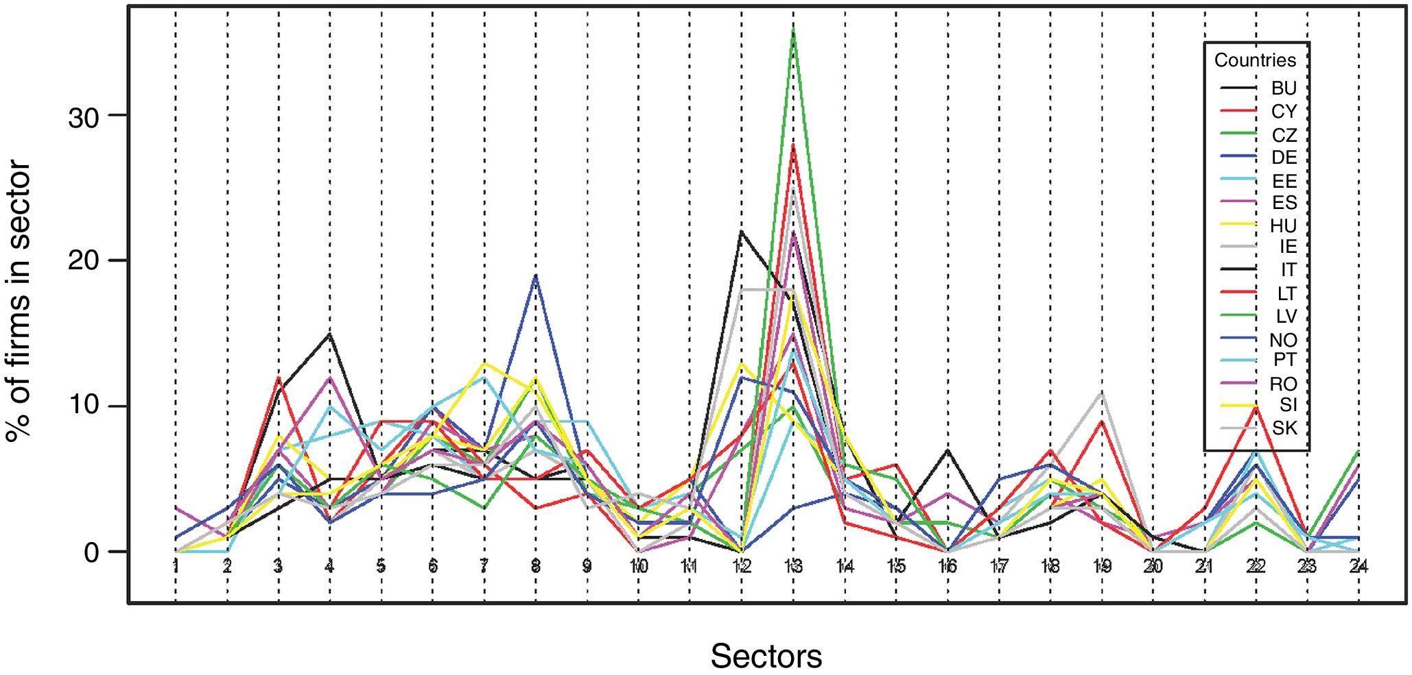
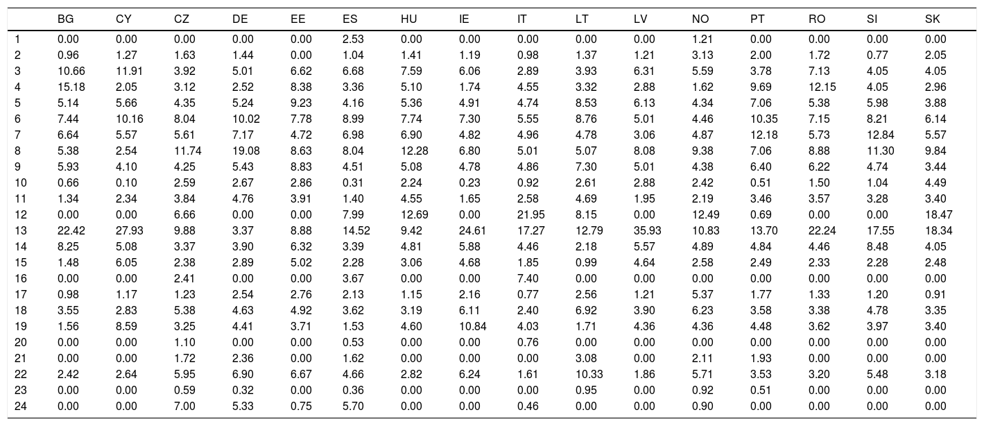
Sector profiles for the 16 countries are presented in the columns of Table 2, and a plot of the 16 profiles is shown in Fig. 3. Equality in the columns of Table 2 implies exact proportionality of the sectors across countries (regardless of whether a country is over- or under-represented in the sample). This equality is not present in our database. For example, sector 13 (Wholesale trade) has a value of 36% in Latvia, but only 3% in Germany. The same applies when countries replace sectors.

Table 2.

Sector profiles in sample size by country (for each sector, % of number in each country).

	BG	CY	CZ	DE	EE	ES	HU	IE	IT	LT	LV	NO	PT	RO	SI	SK
1	0.00	0.00	0.00	0.00	0.00	2.53	0.00	0.00	0.00	0.00	0.00	1.21	0.00	0.00	0.00	0.00
2	0.96	1.27	1.63	1.44	0.00	1.04	1.41	1.19	0.98	1.37	1.21	3.13	2.00	1.72	0.77	2.05
3	10.66	11.91	3.92	5.01	6.62	6.68	7.59	6.06	2.89	3.93	6.31	5.59	3.78	7.13	4.05	4.05
4	15.18	2.05	3.12	2.52	8.38	3.36	5.10	1.74	4.55	3.32	2.88	1.62	9.69	12.15	4.05	2.96
5	5.14	5.66	4.35	5.24	9.23	4.16	5.36	4.91	4.74	8.53	6.13	4.34	7.06	5.38	5.98	3.88
6	7.44	10.16	8.04	10.02	7.78	8.99	7.74	7.30	5.55	8.76	5.01	4.46	10.35	7.15	8.21	6.14
7	6.64	5.57	5.61	7.17	4.72	6.98	6.90	4.82	4.96	4.78	3.06	4.87	12.18	5.73	12.84	5.57
8	5.38	2.54	11.74	19.08	8.63	8.04	12.28	6.80	5.01	5.07	8.08	9.38	7.06	8.88	11.30	9.84
9	5.93	4.10	4.25	5.43	8.83	4.51	5.08	4.78	4.86	7.30	5.01	4.38	6.40	6.22	4.74	3.44
10	0.66	0.10	2.59	2.67	2.86	0.31	2.24	0.23	0.92	2.61	2.88	2.42	0.51	1.50	1.04	4.49
11	1.34	2.34	3.84	4.76	3.91	1.40	4.55	1.65	2.58	4.69	1.95	2.19	3.46	3.57	3.28	3.40
12	0.00	0.00	6.66	0.00	0.00	7.99	12.69	0.00	21.95	8.15	0.00	12.49	0.69	0.00	0.00	18.47
13	22.42	27.93	9.88	3.37	8.88	14.52	9.42	24.61	17.27	12.79	35.93	10.83	13.70	22.24	17.55	18.34
14	8.25	5.08	3.37	3.90	6.32	3.39	4.81	5.88	4.46	2.18	5.57	4.89	4.84	4.46	8.48	4.05
15	1.48	6.05	2.38	2.89	5.02	2.28	3.06	4.68	1.85	0.99	4.64	2.58	2.49	2.33	2.28	2.48
16	0.00	0.00	2.41	0.00	0.00	3.67	0.00	0.00	7.40	0.00	0.00	0.00	0.00	0.00	0.00	0.00
17	0.98	1.17	1.23	2.54	2.76	2.13	1.15	2.16	0.77	2.56	1.21	5.37	1.77	1.33	1.20	0.91
18	3.55	2.83	5.38	4.63	4.92	3.62	3.19	6.11	2.40	6.92	3.90	6.23	3.58	3.38	4.78	3.35
19	1.56	8.59	3.25	4.41	3.71	1.53	4.60	10.84	4.03	1.71	4.36	4.36	4.48	3.62	3.97	3.40
20	0.00	0.00	1.10	0.00	0.00	0.53	0.00	0.00	0.76	0.00	0.00	0.00	0.00	0.00	0.00	0.00
21	0.00	0.00	1.72	2.36	0.00	1.62	0.00	0.00	0.00	3.08	0.00	2.11	1.93	0.00	0.00	0.00
22	2.42	2.64	5.95	6.90	6.67	4.66	2.82	6.24	1.61	10.33	1.86	5.71	3.53	3.20	5.48	3.18
23	0.00	0.00	0.59	0.32	0.00	0.36	0.00	0.00	0.00	0.95	0.00	0.92	0.51	0.00	0.00	0.00
24	0.00	0.00	7.00	5.33	0.75	5.70	0.00	0.00	0.46	0.00	0.00	0.90	0.00	0.00	0.00	0.00

Figure 3.

Profile graph: sector profiles by countries.

A statistical test of the null hypothesis of no confounding (i.e., independence among rows and columns) is the chi-square test of independence presented in Table 1. This test yields χ² = 38,050, df = 345 (p-value < 0.001); thus, the null hypothesis of independence is clearly rejected (the p-value is less than 5%). A statistic of association within the range 0 to 1 is the Pearson's contingency coefficient (pcc),⁹ which in our case takes the value 0.476, a fairly large value, thus indicating a high degree of confounding between country and sectors.

In sum, we find confounding between country and sector, but we do not yet know which countries (sectors) contribute most to this confounding. This issue is addressed in the following subsection.

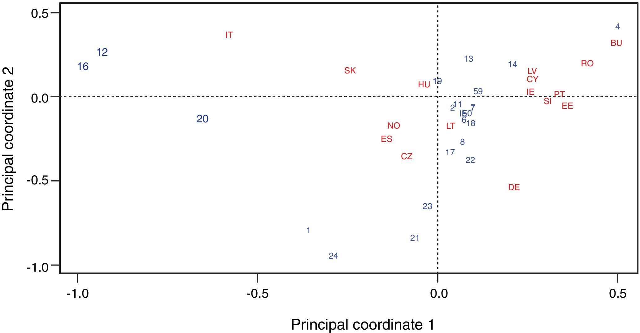
Correspondence analysis

To further examine and disentangle which countries and sectors contribute most to the confounding, we perform correspondence analysis (CA) (e.g., Bartholomew et al., 2000, Chapter 4; Greenacre, 1983; Michailidis and de Leeuw, 1998) based on the contingency table presented in Table 1. CA is a technique that provides a visual representation of the similarity/differences among the 16 sector profiles shown in Fig. 3. In this application, an exact representation would require plotting the sectors as points in a space of dimension equal to the number of countries minus one (i.e., dimension 15). Fig. 4 is an optimal projection in two dimensions of that high dimensional plot. The x- and y-axes of the graph are principal coordinates explaining 40.9% and 26.9% of the profile variation, respectively. Since the x- and y-axes are orthogonal, the chart explains 67.8% (= 40.9% + 26.9%) the overall variation of sectors (idem country) profiles.

Figure 4.

CA plot of countries and sectors.

The CA plot in Fig. 4 is interpreted as follows. Countries close to the centre are characterized by having a sector profile close to the average of all the countries, whereas countries far from the centre represent deviations from the average profile. In addition, countries that are close together indicate similarity in the corresponding profiles (regardless of whether or not they are close to the centre). In our example, Italy, which is positioned on the left side of the scatterplot, has over-representation of sectors 12 (Construction) and 16 (Accommodation and food service activities) but under-representation of sector 4 (Manufacture of textiles, wearing apparel and leather), which lies at the other side of the graph. In contrast, Bulgaria, at the far right of the graph, has under-representation of sectors 12 and 16 and over-representation of sector 4.

To summarize, the graphical representation of the CA plot in Fig. 4 should help researchers to decide how to pool data across countries and sectors. For instance, pooling countries that are close to the centre of the CA plot should prevent confounding in sample size representation among sectors and countries. Similarly, leaving out countries at the extremes of the CA plot also prevents confounding. This approach leads us to RP2:

• •

  Recommended practice 2 (RP2): Examine the sources of the confounding of two domain factors (e.g., in our example, country and sector) using the profile graph and the CA plot, as in Figs. 3 and 4. Care should be taken not to pool data from domains that are observed to contribute highly to confounding.

Missing data

A problem that is often ignored in the practice of statistical analysis is the presence of missing data. This problem is especially acute when analysing large databases, since the number of missing values and the probability of missing data for some variables increases with the size of the dataset (Fernstad and Glen, 2014).

Although numerous studies in the statistical literature caution that missing data is a serious source of bias (e.g., Schafer and Graham, 2002; Tsikriktsis, 2005), missing data problems are usually ignored in the practice of organizational research. The user is often oblivious to the presence of missing data due to the ‘silent’ (without warning) suppression of all the cases that have missing data in any of the variables. In the missing data literature (Little and Rubin, 2014; Rubin, 1976; Schafer, 1997) this approach to the missing data problem is known as listwise deletion, the default option in most statistical software packages. This is clearly a reasonable option when the number of cases suppressed is small. However, when a large number of cases is suppressed, listwise deletion can cause severe distortion in the statistical analysis. Two types of distortions can arise: (a) an increase in the standard errors (thus, a decrease in the power of the tests) due to the elimination of sample information; and (b) bias in the estimates of means, regression coefficients and other parameters of the model due to bias in the sample caused by the case suppression. The latter problem (b) is more serious than the former (a) since it affects not only the precision of the estimates, but also their consistency.

Another popular default option in the software for computing statistics like covariances and correlations is pairwise deletion, which uses all the cases available for computing a sample statistic. For example, in the case of computing the covariance between variables X and Y, all the cases with complete information on X and Y are used. The pairwise option alleviates the above-mentioned problem (a) of reduced sample size since it uses more data information than the listwise option. Problem (b), however, may still persist to some degree. The pairwise option has the added problem that the concept of overall sample size is lost, since the sample size changes for each pair of variables. Other simple options for missing data, for example, mean substitution and hot-deck imputation, are described elsewhere in the missing data literature (see Roth, 1994; Schafer and Graham, 2002; Schlomer et al., 2010; Stumpf, 1978; Tsikriktsis, 2005).

An important concept in the missing data problem is the mechanisms that lead to missing values. In his seminal paper, Rubin (1976) develops a typology of missing data mechanisms: missing completely at random (MCAR), when the probability of missing data is unrelated to the value of the variable itself and to the values of any other variables in the data set; missing at random (MAR), when the probability of missing data does not depend on the value of the variable after controlling for other variables in the dataset; and missing not at random (MNAR), when the presence of missing data in a given position depends on the actual value being missed after controlling for the observables in the dataset (see Allison, 2001, Chapter 2; Little and Rubin, 2014, Chapter 1; Schafer, 1997; Schafer and Graham, 2002). An important result is that under MCAR both listwise and pairwise options are not affected by problem (b) of sample bias; however, under MAR and/or MNAR both listwise and pairwise options can be seriously affected by problem (b). The good news, however, is that in the case of MAR, statistical methods that correct problem (b) are now available to practitioners: one approach is the maximum likelihood for MAR (ML-MAR); another approach is the multiple imputation (MI) procedure. While the ML-MAR requires modifying the standard likelihood function to be maximized, the MI procedure uses a simple three step procedure: (1) produce several complete datasets (i.e., without missing data) by simulation from the distribution of missing values conditional to the observed data; (2) analyse each ‘complete’ dataset using the standard software; finally, (3) average the estimates of the ‘complete’ data analyses using specific formulas. For details of the MI approach, see Allison (2000), and Little and Rubin (2014, Chapter 5). The ML-MAR approach is currently available in the structural equation modelling software (e.g., AMOS, EQS, Lavaan, Lisrel, Mplus, sem of Stata). General statistical software such as SPSS offers ML-MAR to compute covariance and correlation matrices. The MI option is available in the majority of the regression methods in Stata (Stata Corp, 2017). The treatment of missing data in the case of MNAR requires specific modelling outside the standard techniques (Schafer and Graham, 2002; Little and Rubin, 2014). In the present context of large a database, we need to assess the presence of missing data.

It is our view that missing data must be taken into account in the practice of organizational research. A literature search of the published articles using the CIS database found that most articles adopt the listwise deletion option. The few exceptions that have dealt with missing data issues (e.g., Frenz and Ietto-Gillies, 2009; Gelabert et al., 2009) focus on avoiding problems of sample selection bias.

The following subsections present MEDA methods that help to explore missing data patterns and assess the severity of missing data in our database.

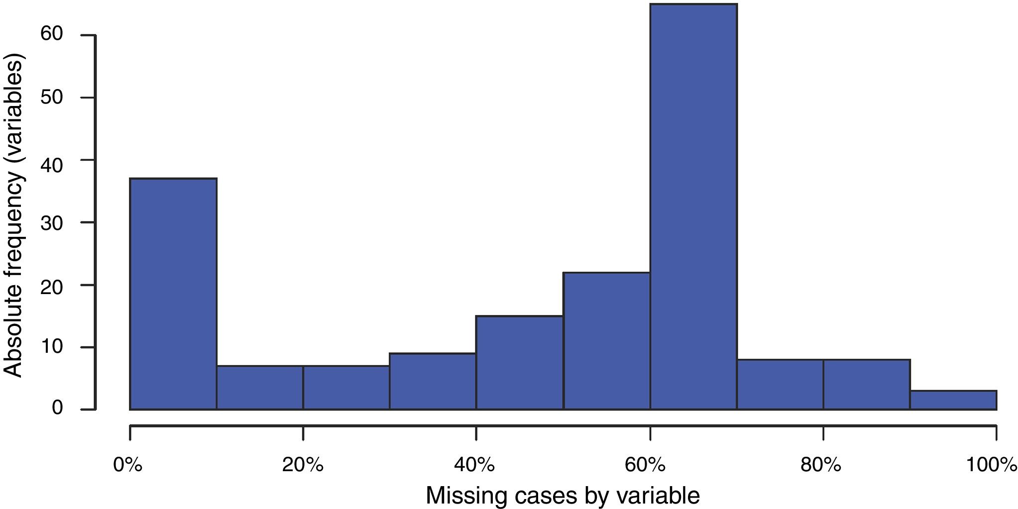
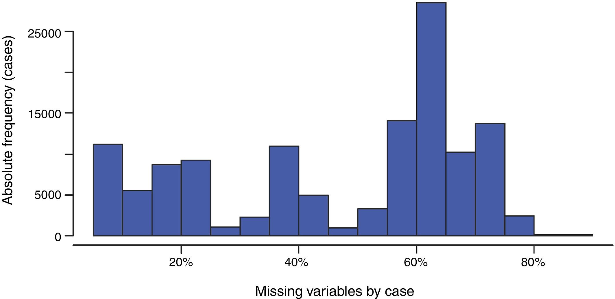
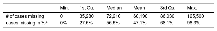
Missing data in cases and variables

An initial assessment of the severity of the missing data problem in a large database involves examining two simple distributions: (1) the distribution of missing cases per variable, and (2) the distribution of the missing variables per case. The histogram of these two distributions in our database is shown in Figs. 5 and 6. Tables 3 and 4 present summary statistics of the distributions.

Figure 5.

Histogram of the percentage of missing cases by variables.

Figure 6.

Histogram of the percentage of missing variables by cases.

Table 3.

Summary statistics for cases missing in variables.

	Min.	1st Qu.	Median	Mean	3rd Qu.	Max.
# of cases missing	0	35,280	72,210	60,190	86,930	125,500
cases missing in %^a	0%	27.6%	56.6%	47.1%	68.1%	98.3%

a

% computed over the total sample size of n = 127,674.

Table 4.

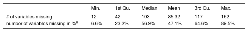
Summary of number of variables missing in cases.

	Min.	1st Qu.	Median	Mean	3rd Qu.	Max.
# of variables missing	12	42	103	85.32	117	162
number of variables missing in %^a	6.6%	23.2%	56.9%	47.1%	64.6%	89.5%

a

% computed over 181, the total number of variables.

Fig. 5 and Table 3 show that 65 out of 181 variables have a high percentage of missing data (around 70%), while fewer than 40 variables present a percentage of missing data below 5%. While some variables have no missing values, other variables have as many as 125,500 cases missing (i.e., 98% cases missing). Note that the distribution is skewed to the left, as the mean is smaller than the median; i.e., the proportion of variables with large numbers of missing cases is greater than those with smaller numbers of missing cases. This table should alert us to the seriousness of missing data in our database.

The histogram in Fig. 6 shows that there are a high number of cases (more than 25,000) with a high percentage (around 70%) of missing variables. Table 4 also reveals that all the cases in our database have a variable missing, in some cases as many as 162 (out of 181). The median of variables missing per case is 103 (more than 50% of missing values), with a mean value of 85.32 (approximately 47%) variables missing per case. Again, these figures should alert us to the seriousness of missing data in our database.

We see that in this database, the listwise option would have serious consequences for the analysis, since a large number of cases (firms) would be excluded. For instance, an analysis involving the 81 variables of model 3 in Table 9 (see the subsection titled Tobit regression below) would imply a reduction in the sample size from 127,674 to 14,420 observations, a reduction that could undermine the representativeness of the analysed sample. This leads us to RP3:

• •

  Recommended practice 3 (RP3): Prior to modelling, it is helpful to report on the distributions of missing cases per variable and missing variables per case, as in Figs. 5 and 6 and Tables 3 and 4 above. These should alert the researcher to the severity of the problem of missing data when using the listwise option.

Missing data across variables

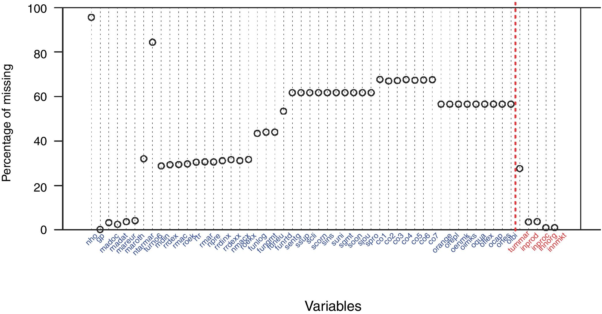
In addition to the simple overall description of the presence of missing data, we display the intensity of missing data across variables. This can be accomplished with a simple scatterplot, such as the one in Fig. 7 that shows the missing cases across variables, represented as dots in the graph. The x-axis displays the names of the variables, and the ordinate of the dot is the percentage of missing cases in the variable. It is a simple task to order the variables in the x-axis according to their subject contents. In our example, the same order as in the questionnaire provides this display. A vertical dotted line separates the demographic and innovation-related covariates (left-hand side) from the dependent variables (right-hand side).

Figure 7.

Missing cases by variable.

It is evident from Fig. 7 that the demographic variables (the first variables in the display) have a very low percentage of missingness. The innovation-related variables, however, have percentages of missing data greater than 50%. Those percentages represent a large amount of missing data, which significantly reduces the effective sample size in the analyses involving these variables if the listwise option is applied. Fig. 7 also shows how some variables have very similar numbers of missing data cases that could be explained by branching and other structures in the questionnaire. To help understand the variation of missing data across variables we propose RP4:

• •

  Recommended practice 4 (RP4): In the case of a severe presence of missing data, it is useful to examine the missing cases by variable plot, as in Fig. 7. This graph helps to identify which variables are most affected by missing values, and to understand the nature and the structure of the questionnaire that produces the database (branching on survey questions, etc.).

Fig. 7 also suggests a limited number of patterns of missing data. The visualization of these patterns is explored in the next subsection.

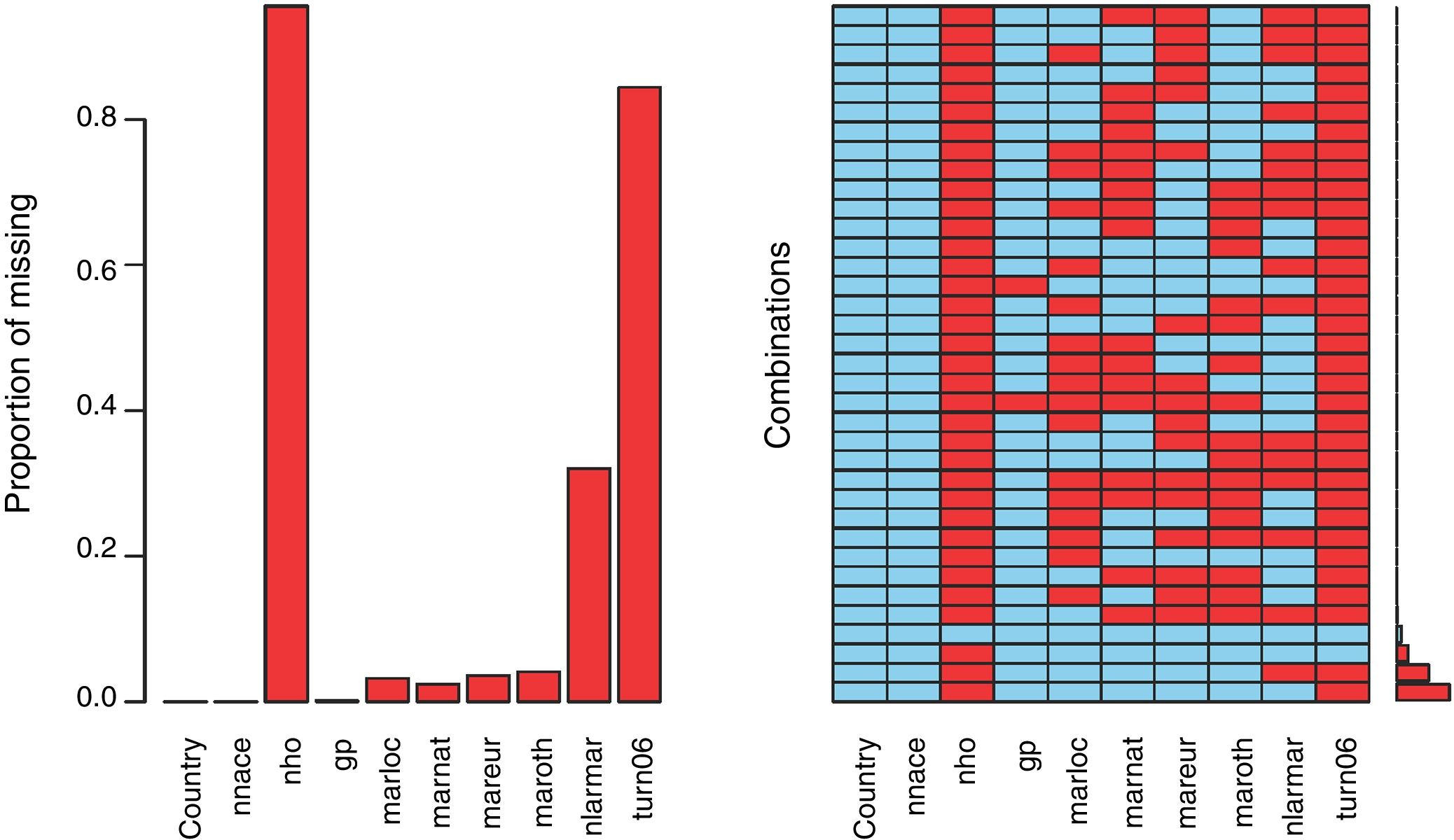
Patterns of missing data for a subset of variables

In some settings, only a subset of variables from the database is used in a specific statistical analysis. In our database, for example, the demographic covariates country, nnace, ho, gp, marloc, marnat, mareur, maroth, and larmar and turn06 are regarded as potential determinants of firms’ innovation. These variables are expected to be observed for all of the firms; in practice, however, they suffer from missing data,¹⁰ so before performing a regression analysis, the magnitude of the missing data problem for these variables must be evaluated. Missing data can be examined using the aggregation plot for missing data shown in Fig. 8.¹¹

Figure 8.

Aggregation plot for missing data on the set of covariates.

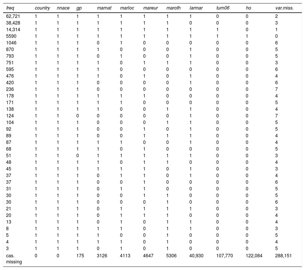
The figure provides summary information about the proportion of missing data by variable (left-hand-side plot), in addition to the patterns of missing data combinations of variables (the right-hand-side plot of the figure). The graph clearly shows variations in the number of missing values per variable, with the highest percentage of missing data corresponding to the variables turn06, larmar and ho. Note that the histogram in the right-hand-side plot of Fig. 8 displays the frequency of the different patterns. An alternative to this histogram is Table 5, which lists the different patterns of missing data in the set of variables. In parallel with Fig. 8, Table 5 shows that the most frequent patterns of missing data are those with missing data in the variables turn06 and ho (of 62,721 cases), larmar, turn06, and ho (with 38,428 cases), and ho (14,314 cases). The fourth largest pattern of missing data (of 5590 cases) is that in which all the variables are observed. This suggests that excluding the covariates turn06, larmar, and ho would prevent a large loss of cases (in a listwise option).

Table 5.

Patterns of missing data on the set of demographic covariates.

freq	country	nnace	gp	marnat	marloc	mareur	maroth	larmar	turn06	ho	var.miss.
62,721	1	1	1	1	1	1	1	1	0	0	2
38,428	1	1	1	1	1	1	1	0	0	0	3
14,314	1	1	1	1	1	1	1	1	1	0	1
5590	1	1	1	1	1	1	1	1	1	1	0
1046	1	1	1	0	1	0	0	0	0	0	6
870	1	1	1	1	0	0	0	1	0	0	5
793	1	1	1	0	1	0	0	1	0	0	5
751	1	1	1	1	0	1	1	1	0	0	3
595	1	1	1	1	0	0	0	0	0	0	6
476	1	1	1	1	0	1	0	1	0	0	4
420	1	1	1	0	0	0	0	1	0	0	6
236	1	1	1	0	0	0	0	0	0	0	7
178	1	1	1	1	1	1	0	0	0	0	4
171	1	1	1	1	1	0	0	0	0	0	5
138	1	1	1	1	0	0	1	1	0	0	4
124	1	1	0	0	0	0	0	1	0	0	7
104	1	1	1	0	0	0	1	1	0	0	5
92	1	1	1	0	0	1	0	1	0	0	5
89	1	1	1	0	0	1	1	1	0	0	4
87	1	1	1	1	1	0	0	1	0	0	4
68	1	1	1	1	0	1	0	0	0	0	5
51	1	1	0	1	1	1	1	1	0	0	3
48	1	1	1	1	0	1	1	0	0	0	4
45	1	1	1	1	1	1	0	1	0	0	3
37	1	1	1	0	1	1	0	1	0	0	4
37	1	1	1	0	0	1	0	0	0	0	6
31	1	1	1	0	1	1	0	0	0	0	5
30	1	1	1	0	0	1	1	0	0	0	5
30	1	1	1	0	0	0	1	0	0	0	6
21	1	1	1	0	1	1	1	1	0	0	3
20	1	1	1	0	1	1	1	0	0	0	4
13	1	1	1	0	1	0	1	1	0	0	4
8	1	1	1	1	1	0	1	1	0	0	3
5	1	1	1	1	0	0	1	0	0	0	5
4	1	1	1	1	1	0	1	0	0	0	4
3	1	1	1	0	1	0	1	0	0	0	5
cas. missing	0	0	175	3126	4113	4647	5306	40,930	107,770	122,084	288,151

The above graph should help researchers in their choice of the method to deal with missing data. For example, to exclude certain variables from the initially specified set, if it does not defeat the purpose of the analysis, apply modern methods of missing data such as ML-MAR or MI. This situation leads us to RP5:

• •

  Recommended practice 5 (RP5): When a subgroup of variables is entered into a specific analysis, it is important to examine the patterns of missing data in the subgroup. This examination can be made using the aggregation plot for missing data in Fig. 8 and/or the patterns of missing data in Table 5. Under the listwise option the plot suggests which variables should be excluded to avoid a large loss of cases. Alternatively, if none of the variables can be excluded (due to their relevance in the analysis), then other missing data options such as ML-MAR or MI should be adopted.

Dimension reduction

The main purpose of using the CIS database is to find determinants (explanations) for firm innovation. In the database, innovation is associated with two types of variables: four binary variables that report the presence in the firm of a type of innovation during the period of observation (inprod, inproc, inorg and inmkt) and, for firms that innovate in new products, a continuous variable (turnmar), which measures the percentage of total turnover of the firm that is accounted for by new-to-the-market products. One option is to perform a logistic regression for each of the four binary variables. Instead, given the association among the four binary variables, an alternative is to construct an innovation index to be used as the dependent variable in a regression equation.

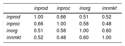
Dimension reduction of dependent variables

Extraction of an index is justified by the assumption of communality among the four types of innovations, represented by the four binary variables inprod, inproc, inorg and inmkt. Table 6 reports the Pearson's contingency coefficient (pcc) among the four indicators. The values yielded are high, most of them above 0.5, indicating high communality among the four types of innovations. Several multivariate scaling techniques could be used to reduce the four dependent variables to a single index. Dimension reduction techniques, such as principal component analysis (PCA), exploratory or confirmatory factor analysis (FA), or frontier methodologies,¹² could be applied to construct a one-dimensional index of innovation.¹³ Discussion on the quality of the different methods for data reduction is beyond the scope of the paper. The decision of which method for scaling is most suitable on specific research context should be based on both theoretical (the meaning attributed to the index) and empirical (e.g., dimensionality and reliability of the measures) arguments. Often, simple indices (this is the case of the sum in our example in Section “Discussion”) are good summaries of a correlated set of variables. This approach leads us to propose RP6:

• •

  Recommended practice 6 (RP6): In the case of multiple dependent variables that are highly associated, as in Table 6, dimension reduction should be applied to the set of dependent variables. This dimension reduction can be undertaken using substantively motivated indices, or dimension reduction by principal component or factor analysis methods. In this way, the multivariate response can be reduced to a univariate regression model, thus facilitating interpretation of analysis.

Table 6.

Pearson's contingency coefficient among types of innovations.

	inprod	inproc	inorg	innmkt
inprod	1.00	0.66	0.51	0.52
inproc	0.66	1.00	0.58	0.48
inorg	0.51	0.58	1.00	0.60
innmkt	0.52	0.48	0.60	1.00

RP6 would also apply when the multivariate dependent vector is not discrete but continuous. In this case, Table 6 would report Pearson's correlation coefficients instead of Pearson's contingency coefficients.

A related situation in which high correlations are a problem concerns their presence in the set of covariates. We explore this issue in the following subsection.

Dimension reduction of covariates

The set of covariates used in the analysis may pose a problem when the covariates are closely associated since this situation can lead to severe multicollinearity problems. The association should therefore be examined. In our CIS example, we use the following demographic covariates: country, nnace, gp, marloc, marnat, mareur, and maroth, the same variables that were examined for missing data in the previous section.¹⁴

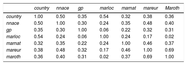
Before any regression equation is estimated with these covariates, the association among them needs to be assessed. Table 7 shows the pcc for these variables (if the variables had been continuous, the Pearson correlation coefficient would have been used). Different levels of association between the variables can be seen in the table: a low association (pcc = 0.02) between marloc (local market) and maroth (other non-European countries), but a higher association (pcc = 0.24) between marloc and marnat (national market). The association between country and marloc (pcc = 0.54) is also high, the reason being that in some countries, firms focus more on the local market (i.e., have a lower export orientation) than in others. Finally, we also see a high association between country and sector (nnace), that is, there is a high association between countries and type of industries (pcc = 0.5). An exploratory analysis of the association between the covariates may thus provide useful insights for the selection of the set of covariates in the regression equation, or regarding the need to conduct dimension reduction on sets of covariates. Section “Ordered logistic regression” provides a specific example of covariate dimension reductions in a ordered logistic regression analysis. This leads us to RP7:

• •

  Recommended practice 7 (RP7): Before fitting a regression model with many covariates, association among sets of covariates should be assessed. If high association is present, then summary indices (as in RP6) among subsets of covariates should be constructed. Reducing the number of covariates via the indices should help to avoid multicollinearity problems.

Table 7.

Pearson's contingency coefficient among covariates.

	country	nnace	gp	marloc	marnat	mareur	Maroth
country	1.00	0.50	0.35	0.54	0.32	0.38	0.36
nnace	0.50	1.00	0.30	0.24	0.35	0.48	0.40
gp	0.35	0.30	1.00	0.06	0.22	0.32	0.31
marloc	0.54	0.24	0.06	1.00	0.24	0.17	0.02
marnat	0.32	0.35	0.22	0.24	1.00	0.46	0.37
mareur	0.38	0.48	0.32	0.17	0.46	1.00	0.69
maroth	0.36	0.40	0.31	0.02	0.37	0.69	1.00

The usefulness of the above RPs is illustrated in the next sections in which we model innovation performance using the CIS database.

Modelling innovation: an illustration

This section discusses modelling innovation performance using the CIS data presented earlier. The MEDA methods discussed above clarify that the CIS database involves several binary variables accounting for whether or not the firm is involved in several types of innovations. In addition, other variables inform on the intensity of the innovation activity of the firms engaged in product innovation. The CIS database also contains a set of innovation-related variables (activities promoting innovation in the firm), and two variables that classify the firms in different countries and sectors. This leads us to discuss two models: one for the index of innovation constructed with binary variable indicators of the innovation types (inprod, inproc, inorg and inmkt); and a second modelling the intensity of product innovation performance. As mentioned in Section “The Community Innovation Survey”, two variables measure the intensity of product innovation: turnmar (percentage of total turnover from product innovations that are new to the market) and turnin (percentage of total turnover from product innovations that are only new to the firm). For the sake of brevity in the illustration, we do not include the variable turnin. The same analysis as for turnmar would apply when turnin is used as dependent variable.

Attending to the level of measurement of the variables, an ordered logistic regression is proposed in the case of the index of innovation, and a Tobit regression model for the variable turnmar. In this modelling exercise, we adhere to the proposed RPs to solve the statistical complexities of the database described in the previous sections, such as dimension reduction and missing data.

Ordered logistic regression

Assessing the determinants of the types of innovation in our database calls for logistic regression, with one regression equation for each innovation type. However, following RP7, Table 6 identifies a high association among the types of innovations. To explain this association, RP7 proposed building an index of innovation that captures the communality of the different innovation types. We use the simple approach of defining the index just as the sum of the four variables (as mentioned in RP7, alternatives for index construction such as PCA and FA with continuous or discrete data could have been used).¹⁵ In this section, we use the index of innovation as the dependent variable in the regression equation, as an alternative to the fourth logistic regression on the binary variables inprod, inproc, inorg, and inmkt.¹⁶ Note that attending to RP2, which pointed to the high association between country and sector, we will include both factors in the regression model.

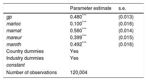
The results of the ordered logistic regression are shown in Table 8. The table presents the regression coefficients of the covariates, once the effects of countries and sectors are controlled for (their regression coefficients will be shown in Figs. 9 and 10). All the covariates are highly significant. In fact, the high significance of all the regression coefficients is what should be expected with a large dataset in terms of number of cases such as the one used in this model (where n = 120,004).

Table 8.

Results of the ordered logistic regression of innovation on covariates. (The regression coefficient for dummy variables of country and sector are not shown in the table.).

	Parameter estimate	s.e.
gp	0.480^***	(0.013)
marloc	0.100^***	(0.016)
marnat	0.560^***	(0.014)
mareur	0.399^***	(0.015)
maroth	0.492^***	(0.016)
Country dummies	Yes
Industry dummies	Yes
constant
Number of observations	120,004

***

p < 0.01.

Figure 9.

Regression estimates for country dummies.

Figure 10.

Regression estimates for sector dummies.

Fig. 9 reports the regression coefficients of the country dummies that were not shown in Table 8. The graph shows highly positive performance for Latvia and the Czech Republic, but Spain and Slovakia have negative coefficients (note that the country of reference is Bulgaria). These regression coefficients correspond to the country innovation performance once we have controlled for sector and the other covariates.

Fig. 10 reports the regression coefficients of the sector dummies that were not shown in Table 8. The graph reveals differences in the innovation intensity across sectors once we have controlled for the covariates. Sectors 13 (Wholesale trade), 14 (Land, water and air transport) and 15 (Warehousing and support activities; Postal and courier activities) are below the zero level, which corresponds to the reference category, sector 1 (Agriculture, forestry and fishing). On the other hand, sectors 18 (Telecommunications), 17 (Publishing activities) are those with higher intensities in innovation performance. This leads to RP8:

• •

  Recommended practice 8 (RP8): In the case of a large number of domain indicators (in a regression equation, countries and sectors), it is helpful to display in a separate graph the regression coefficient of the domain indicators, as illustrated in Figs. 9 and 10. This allows the researcher to visualize variation across domains of the dependent variable after controlling for covariates.

Tobit regression

Thus far, the regression approach has explained innovation using an ordered logistic regression. However, for firms that innovate in new products, e.g., the firms where inprod is equal to 1, the CIS database provides the variable turnmar, a continuous variable that measures the intensity of product innovation.¹⁷ Restricting the analysis to this subset of firms, the initial 127,674 firms in the CIS 2008 database are reduced to 30,630 (the subset of firms where inprod is equal to 1). For those firms, however, the CIS database contains an additional set of innovation-related variables, so the number of covariates increases substantially in this subset of firms. Specifically, there are 40 innovation-related variables available as possible covariates for the regression model. These variables have been described in Section “The Community Innovation Survey” and are listed in Appendix 2; they have also been extensively used in previous studies as determinants of product innovation (e.g., Belderbos et al., 2004; Cesaratto and Mangano, 1993; Hollenstein, 2003; Leiponen and Drejer, 2007; Mention, 2011; Peneder, 2010; Raymond et al., 2004; Tether, 2002, among others). Attending to RP7, this large number of covariates (40 variables) calls for data dimension reduction. This has been accomplished using PCA applied to subsets of covariates, leading to the following summary indices: objectives, sources, cooperation, and support (they correspond, respectively, to the groups (3) to (6) of the innovation related-variables commented in Section “The Community Innovation Survey”).

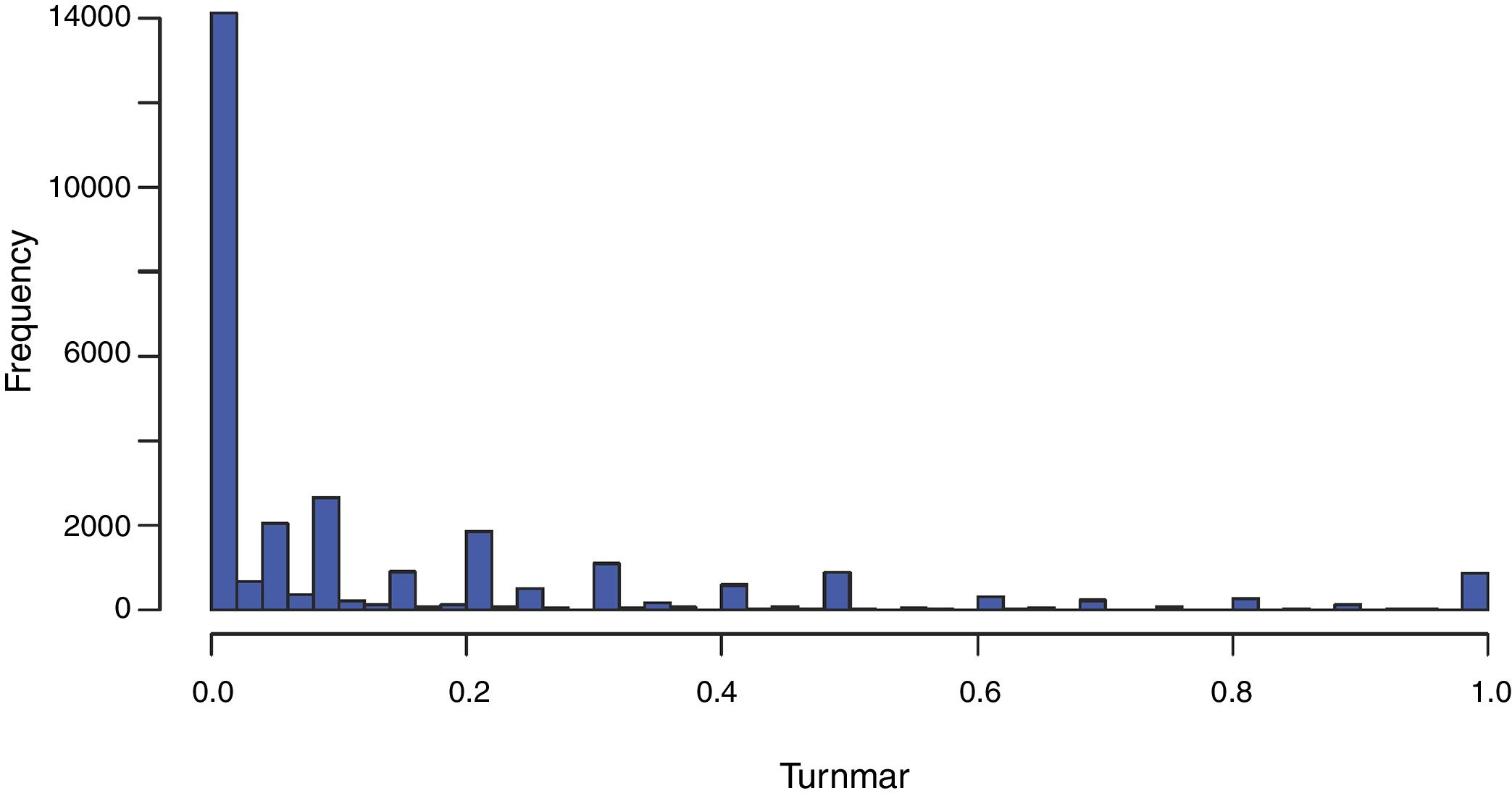
Several relevant statistical issues arise in the regression analysis with dependent variable turnmar. The first one is apparent in Fig. 11, which displays the marginal distribution of the variable turnmar. The histogram shows a high concentration of zeros: specifically, more than 14,000 firms, nearly 50%, have a value of 0. Moreover, linear regression assumes there is no restriction on the values of the dependent variable; but by construction, turnmar is confined to the interval 0–1. The distribution of the variable turnmar calls for a modification of the standard OLS regression model. Following previous studies with CIS data (e.g., Laursen and Salter, 2006; Van Beers and Zand, 2014), we will use censored (Tobit) regression (Tobin, 1958). Other approaches have been used; among others, Heckman selection models (Cerulli and Potì, 2012; Frenz and Ietto-Gillies, 2009; Sapprasert and Clausen, 2012), quantile regression (Segarra and Teruel, 2014), two-stage least-squares regression (Garriga et al., 2013). In this case of a dependent variable with a restricted range, fractional response models have also been proposed (see Wooldridge, 2011).

Figure 11.

Distribution of the dependent variable turnmar (n = 30,630).

An added problem is missing data. Of the 30,630 firms with product innovation, 1568 firms have missing data for the dependent variable turnmar, a percentage of 5.1% that in practice can be ignored; however, as we showed in Fig. 7, the set of the new covariates suffer from a severe problem of missing data (see RP5). Some covariates have missing data for more than 50% of the cases, thus applying listwise deletion in this context would imply suppressing more than half of the cases.

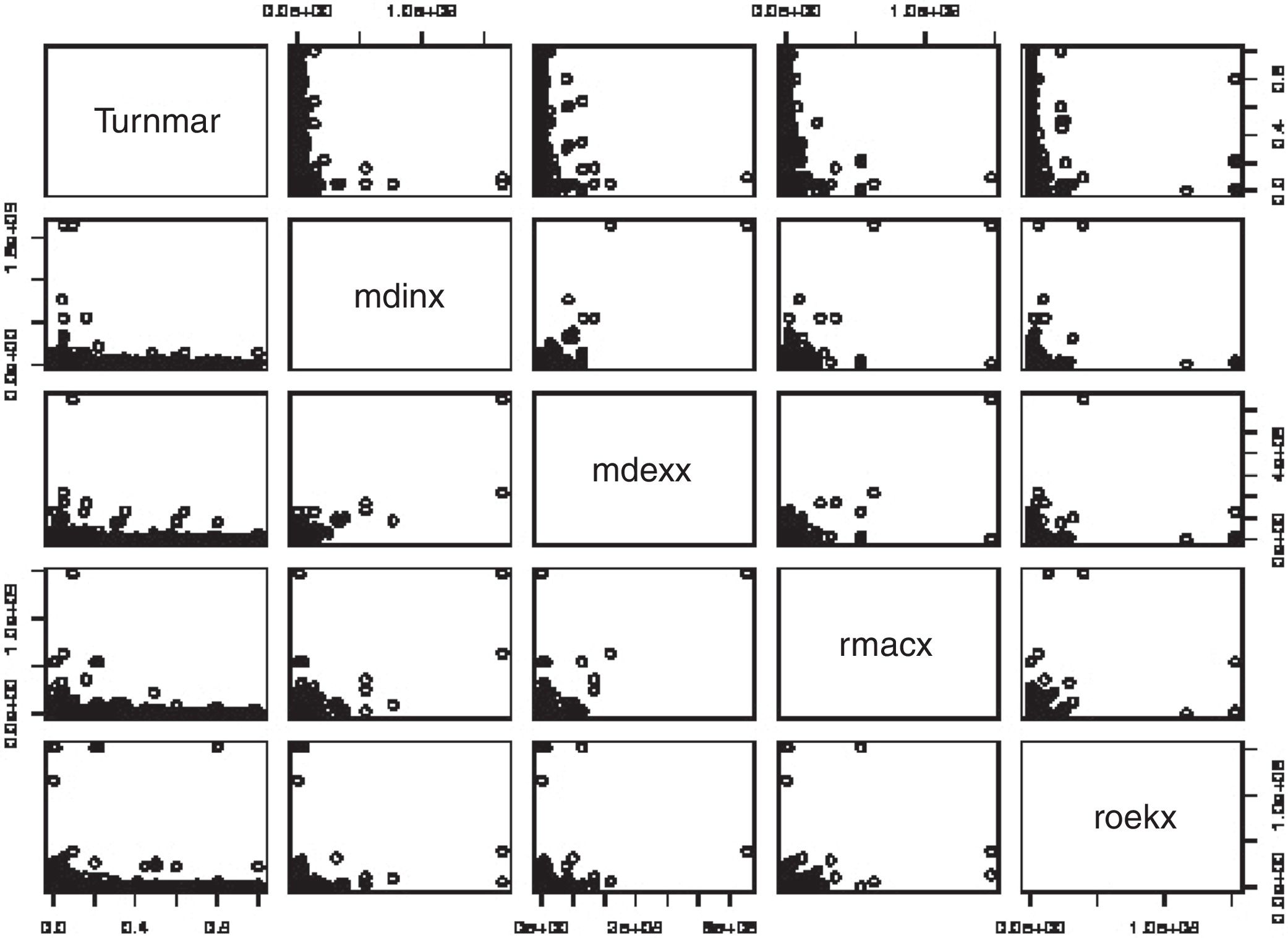
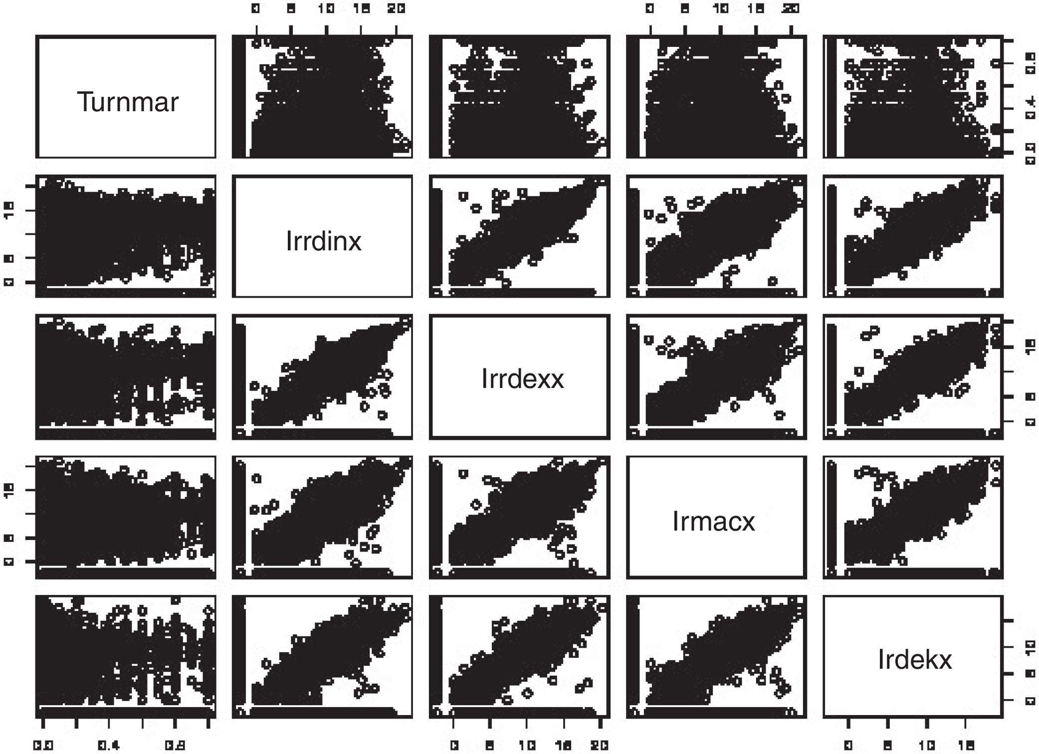
Furthermore, the matrix plot shown in Fig. 12 suggests there is a problem of non-linearity in this regression analysis. Fortunately, in our application log transformation of the covariates solves this non-linearity problem (compare Figs. 12 and 13). The following RP9 is suggested:

• •

  Recommended practice 9 (RP9): When confronted with a continuous dependent variable, its marginal distribution needs to be inspected, such as in Fig. 11. This should help in choosing the most appropriate model, e.g., the choice of Tobit regression instead of OLS. Linearity should also be assessed. This can be accomplished using matrix plots like the ones of Figs. 11 and 12. Deviations from linearity require the transformation of the data. Sometimes, a logarithmic or exponential transformation solves the non-linearity issue.

Figure 12.

Matrix plot without log transformation of covariates.

Figure 13.

Matrix plot with the log transformation of covariates.

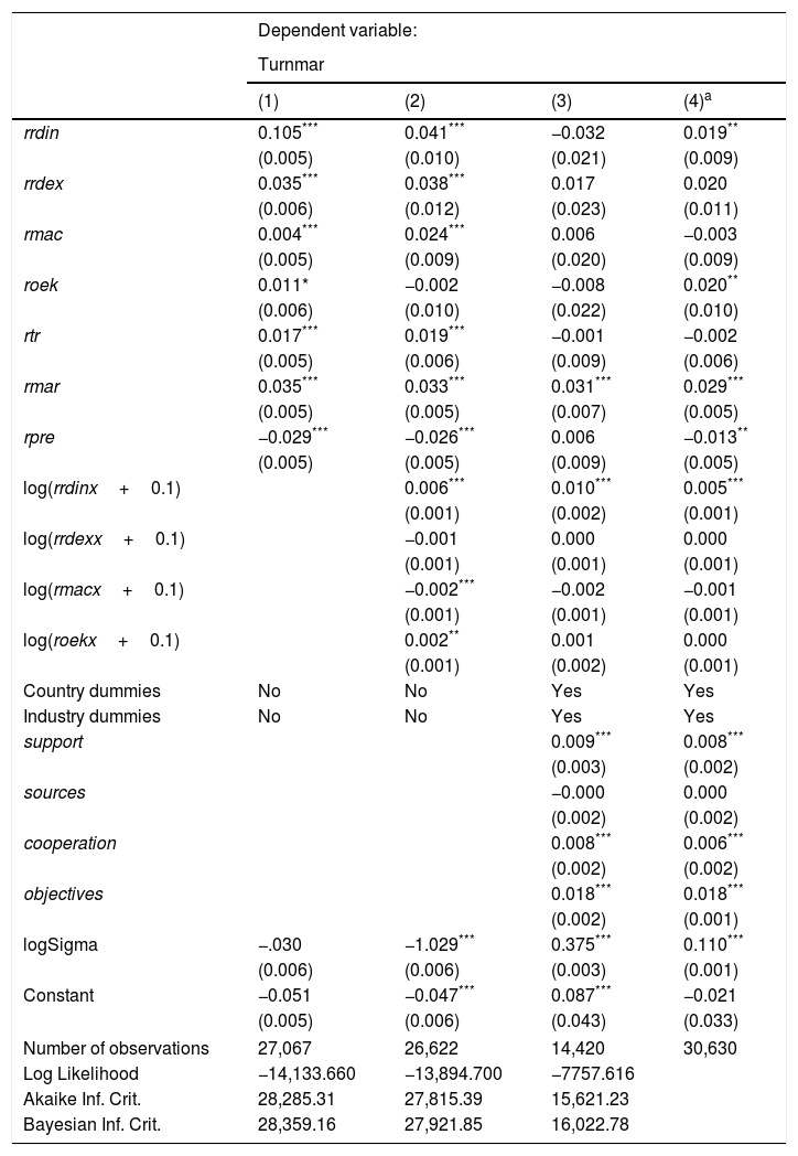
The first three columns of Table 9 shows the estimation results for Tobit regression with increasing number of covariates and using the listwise (default) option for missing data. Note that the listwise option leads to a severe decrease of the sample size when the model expands on covariates. Note that sample size decreased by nearly 50% when moving from the first to the third column of Table 9. Section “Missing data” warned of the potential loss of efficiency when using the listwise option for missing data, and we see, indeed, a substantial increase in standard errors when comparing the estimates of the third model with the previous two. Section “Missing data” also warned of the potential for bias on estimates due to using listwise, but there is no way to have a hint on that by simple inspection of estimates.

Table 9.

Tobit regressions.

	Dependent variable:
	Turnmar
	(1)	(2)	(3)	(4)^a
rrdin	0.105^***	0.041^***	−0.032	0.019^**
	(0.005)	(0.010)	(0.021)	(0.009)
rrdex	0.035^***	0.038^***	0.017	0.020
	(0.006)	(0.012)	(0.023)	(0.011)
rmac	0.004^***	0.024^***	0.006	−0.003
	(0.005)	(0.009)	(0.020)	(0.009)
roek	0.011*	−0.002	−0.008	0.020^**
	(0.006)	(0.010)	(0.022)	(0.010)
rtr	0.017^***	0.019^***	−0.001	−0.002
	(0.005)	(0.006)	(0.009)	(0.006)
rmar	0.035^***	0.033^***	0.031^***	0.029^***
	(0.005)	(0.005)	(0.007)	(0.005)
rpre	−0.029^***	−0.026^***	0.006	−0.013^**
	(0.005)	(0.005)	(0.009)	(0.005)
log(rrdinx + 0.1)		0.006^***	0.010^***	0.005^***
		(0.001)	(0.002)	(0.001)
log(rrdexx + 0.1)		−0.001	0.000	0.000
		(0.001)	(0.001)	(0.001)
log(rmacx + 0.1)		−0.002^***	−0.002	−0.001
		(0.001)	(0.001)	(0.001)
log(roekx + 0.1)		0.002^**	0.001	0.000
		(0.001)	(0.002)	(0.001)
Country dummies	No	No	Yes	Yes
Industry dummies	No	No	Yes	Yes
support			0.009^***	0.008^***
			(0.003)	(0.002)
sources			−0.000	0.000
			(0.002)	(0.002)
cooperation			0.008^***	0.006^***
			(0.002)	(0.002)
objectives			0.018^***	0.018^***
			(0.002)	(0.001)
logSigma	−.030	−1.029^***	0.375^***	0.110^***
	(0.006)	(0.006)	(0.003)	(0.001)
Constant	−0.051	−0.047^***	0.087^***	−0.021
	(0.005)	(0.006)	(0.043)	(0.033)
Number of observations	27,067	26,622	14,420	30,630
Log Likelihood	−14,133.660	−13,894.700	−7757.616
Akaike Inf. Crit.	28,285.31	27,815.39	15,621.23
Bayesian Inf. Crit.	28,359.16	27,921.85	16,022.78

**

p < 0.05.

***

p < 0.01.

a

Tobit regression using multiple imputation (MI) for missing data.

As commented in Section “Missing data”, the MI estimation approach for missing data prevents bias when the missing mechanism is MAR. The MI estimates are presented in column (4) of Table 9; thus, comparison of columns (3) and (4) shows differences in estimation when using two different approaches to missing data. Column (3) is correct only under the strong assumption of non-informative missingness (MCAR); column (4) is correct under the weaker assumption of MAR (recall the discussion in Section “Missing data”). We see that the MI estimates generally show lower standard errors, and the covariates rrdin, roek and rpre are now statistically significant. It would extend beyond the scope of this paper to elaborate more on the differences between the two types of estimates. The important point to note, however, is that indeed, a substantial difference on estimates can arise in practice depending on which treatment we apply to the missing data problem.

Discussion

The paper has illustrated specific MEDA methods that can help organizational researchers to understand the potential and limitations of a large dataset, prior to model fitting. A large database on firms’ innovation, the CIS database, provides the context for the illustration. This is a sampling-based database of firms selected from a population spread over different countries and sectors. The sampling-based characteristic raises issues of representativeness of the sample on the different domains of the population. Issues of missing data and dimension reduction arise naturally when large databases are involved. The following issues were discussed:

• 1.

  Sample size representativeness across multiple domains (in our example, countries and sectors). Graphical tools based on correspondence analysis were used to assess the variation in sample size representativeness across domains.

• 2.

  Assessing the severity of the missing data problem. Methods for handling missing data were discussed, and an application of the MI method for missing data is applied to a Tobit regression with CIS data.

• 3.

  Dimension reduction based on principal component analysis or other methods, for both dependent and subsets of covariates, was also discussed. This simplifies the analysis when dealing with several redundant dependent variables and avoids the multicollinearity problem.

• 4.

  Inspection of the distribution of the dependent variable was advocated to assist in the choice of model to be fitted; e.g., a Tobit regression instead of OLS regression.

• 5.

  Finally, the MEDA methods discussed assisted modelling CIS data using ordered logistic and Tobit regression models using CIS.

We provided a set of recommended practices of MEDA that can assist practitioners in fitting models in a context of a large database. All the methods discussed in this paper can be implemented with standard software used in organizational research (Stata, SPSS, R, etc.). For completeness, Appendix 3 provides the code in R to implement all the analyses in the paper.

The paper has been confined to the MEDA methods that are more directly relevant to the CIS data. Other MEDA methods (e.g., tools for detecting outliers, data-driven clustering of cases and variables, etc.) could also be brought into the discussion, but that this would be beyond the scope of the present paper.

Funding

This work was supported by the Spanish MEC Grants [Grant Number ECO2015-66671-P (MINECO/FEDER), and ECO2014-59885-P] and Generalitat Valenciana [Grant Number BEST/2018/209].

Acknowledgements

The authors thank the European Commission's Eurostat for access to microdata from the Community Innovation Survey 2006 (CIS-2006). Eurostat is not responsible for the results and conclusions of this study.