

Epidemiology is concerned with groups of subjects belonging to populations, not with each individual subject, and takes into account both the subjects who contract a disease and those who do not. Comparison, thus, is a basic element of this discipline.
Measures of frequency, association and impact are the main statistical resources employed in epidemiology to describe the distribution of healthcare problems, establishing a causal relationship between exposure and disease, enabling users to evaluate the impact of preventive measures in the field of public health.
Epidemiology is concerned with groups of subjects belonging to populations, not with each individual subject, and takes into account both the subjects who contract a disease and those who do not. Comparison, thus, is a basic element of this discipline. Information on groups and comparisons between them are based on the prior assumption that health-related problems present a non-random distribution.
Epidemiology has been defined more fully as “the study of the occurrence and distribution of health-related status or events in specified populations, including the study of the determinants influencing such states, and the application of this knowledge to control the health problems”.1
This definition highlights the three levels of response in epidemiologic research: (1) Descriptive level. Describing the distribution of a health problem or disease in relation to the characteristics of the persons, the place and the evolution of the frequency of appearance over time; (2) Aetiology level. Establishing the causal or determinant factors of the disease or health problem being studied; (3) Treatment level. Evaluation of the potential impact of the measures proposed in relation to the health problem or disease.
In each of these epidemiologic response levels, it is necessary to possess objective means of measuring the frequency of the disease, the association between variables and the collective impact of the public health or therapeutic preventive measures taken.2
Measures of Disease FrequencyPoint prevalence (P)This measure quantifies the proportion of subjects presenting the disease at a given moment or period of time. Like all proportions, it has no dimensions and its value lies between [0,1].3
Example 1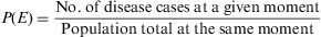
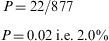
A random sample was taken of 877 young people, aged 15–24 years, resident in city A in southern Spain. On application of the corresponding tests, 22 were diagnosed as being allergic to olive pollen. The prevalence of olive pollen allergy among this group of subjects is then calculated as:
This measure of prevalence - point prevalence, or simply ‘prevalence’ – is the most commonly used, but there are variations, such as:
- a.
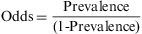
The prevalence odds ratio. This disease frequency measure is calculated by dividing the probability of an event occurring at a specific moment of time (prevalence) by the probability of its not occurring (1- prevalence).
The odds ratio is a proportion with a range from 0 to infinity, and like prevalence it has no time dimension. In the case of the above example, the odds would be 0.02/(1−0.02)=0.02. The odds and the prevalence measure the same effect, but on different scales. The odds ratio is not widely used as a measure of disease frequency, and its interest in epidemiology lies in the fact that it can be determined in case studies with controls, and that it can be easily determined from linear regression models.
- b.
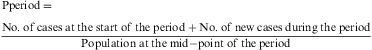
The prevalence by period, or the number of disease cases at any moment during a given period of time. This is relativised by means of the period prevalence ratio, i.e. the probability of any individual within a population constituting a disease case within a given period of time.
This parameter is measured using the ratio between the number of subjects affected by a given phenomenon during an interval of time with respect to the total population size during the same interval. In the case of a fixed cohort, the denominator is the population at the start of the period. If the mid-interval population is not known, it is calculated by interpolation, from the population at the start point and that at the end of the period.
Prevalence measures are useful for the planning and administration of healthcare services, for example in measuring the frequency of remittent diseases and those not identified at the outset. In genetic medicine, in the case of congenital malformations, the normal measure used is that of prevalence, taking into account the fact that malformed neonates constitute those infants capable of surviving their malformation at least until after birth.
IncidenceMeasures of incidence refer to the number of new disease cases appearing during a period of time. There are two types of measures of incidence: accumulated incidence and rate of incidence, or incidence density.4
Accumulated Incidence (AI)This is the proportion of healthy individuals at the start of a given period of time who become ill during the same period. It is calculated as follows:

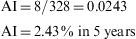
Both the numerator and the denominator include only the cases free of disease at the start of the study period, and therefore cases that are at risk of acquiring the disease. As in the case of prevalence, AI does not have dimensions, and its values range from 0 to 1, expressed as a percentage. To be correctly interpreted, AI must be expressed with reference to the interval of the time period in question.Example 2 During a period of 5 years, a study is made of 326 men aged 30–60 years. All these subjects are healthy and work in a metal-working company. The aim of the study is to detect allergies to steel. At the end of the 5-year period, 8 persons are found to be allergic to steel or related elements. In this case, the accumulated incidence is:
The Accumulated Incidence calculation assumes that the entire population during a given period of time is observed for the whole period of time to detect whether the disease of interest is developed. Nevertheless, in real life what normally happens is that:
- a.
The subjects to be observed enter the study at different moments of time.
- b.
The observation of these subjects is not uniform, as some information is missing in some cases.
- c.
Some subjects abandon the study, and thus the observation period is limited.
ID is not a proportion, but a rate, as the denominator incorporates the dimension of time. Its value cannot be less than zero, but it has no upper limit (i.e. the range is zero to infinity). ID indicates the number of subjects who evolve from a healthy to a diseased state, or vice versa, per unit of time and in relation to the size of the population at risk. The number of healthy individuals who fall sick during any period of time is a product of three factors: the size of the population, the length of the time period and the pathogenic power or morbidity force (characteristic of the disease) acting on the population. ID measures this force; it does not reflect the number of new cases occurring within a given period, but expresses the speed at which a disease develops within a population. It is calculated as follows:
Example 3
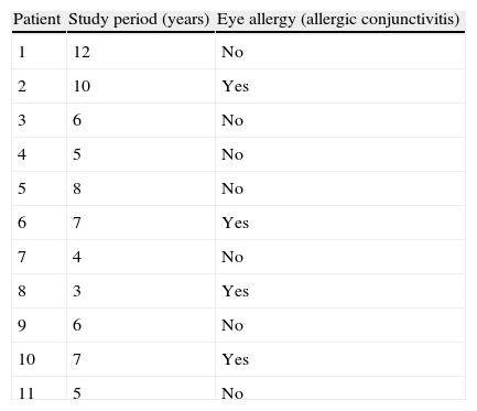
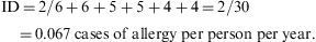
Table 1 shows the results of the observation of 11 patients over a period of 12 years, in a study of the appearance of eye allergies (allergic conjunctivitis).

Thus, the density of ocular allergies (allergic conjunctivitis) in this example is 5.5 new cases per 100 persons per observation year. In other words, the rate at which this group of persons acquires the disease (i.e. the speed of evolution from healthy to sick) is 0.055 per observation year or risk year.Example 4 During the period 1998–2004, a study was made of six women who had suffered an allergy to grasses such as orchard grass (Dactylis glomerata), timothy grass (Phleum pratense), Perennial Ryegrass (Lolium perenne), Kentucky bluegrass (Poa pratensis), Bermuda grass (Cynodon dactylon), etc., to measure the reappearance of this allergy. Two of the six women were observed over the full six years of the study, two for five years, and the remaining two, for four years. In the case, the incidence density is calculated as:
When is it appropriate to use accumulated incidence and when is incidence density more suitable?
ID can be used when the object of the exercise is to study the pattern of evolution of a disease over time, and in relation to the exposure to a risk factor (RF). AI requires, in any study of incidences associated with exposure to RF, that the time of latency of the disease (or incubation period, in the case of infectious diseases), i.e. the time during which the subject is at risk of falling ill following exposure to RF, is both known and lies within the observation period of the study, these being essential conditions for determining the AI denominator.
The choice of one or other of these two measures of incidence depends, as well as on the aims of the study, on the characteristics of the disease to be examined. Thus, AI is generally used when the disease presents a short period of latency, while ID is preferred in the case of chronic illnesses, with a greater period of latency.
One advantage of ID is that it is applicable in conditions in which the population size is fixed, while it can also be used in the case of dynamic or open populations. In the latter case, ID can tolerate the entry and exit of patients throughout the period of observation.
Measures of association or of effectMeasures of association estimate the magnitude of the relation between a factor (exposure) and a health problem or disease (result/outcome).5 Association can be viewed as the statistical dependence between two magnitudes. The principal measures of association are:
Relative RiskThe rate of accumulated incidences is termed the Relative Risk (RR), and is defined as the ratio of the risk of contracting the disease among a group of exposed subjects compared to the risk among a similar group of unexposed subjects. Thus, it is a ratio of two risks.
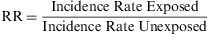
The RR expresses the factor by which the risk or probability of the study event occurring is multiplied within the exposed group, in comparison with the unexposed group. Its value cannot be less than zero, but it has no upper limit. Thus, its range is zero to infinity. When its value is less than 1, there is no association between the exposure and the event; when it is greater than 1, the association is positive, i.e. the exposed group has a greater incidence than the unexposed group has; when it is less than 1, the association is negative (this is also known as the ‘protective effect’).
Prevalence Ratios are estimated and expressed in an analogous way, except that prevalences, rather than accumulated incidences, are used. Both Relative Risks and Prevalence Ratios must be accompanied by the calculations of their respective confidence intervals (normally calculated at 95%) in order to determine the precision of the values presented.
The Incidence Density Ratio (IDR) or Rate Ratio is defined as the ratio of the incidence density of an exposed group to that of an unexposed one. It expresses how many times the event occurs with greatest speed among persons exposed, in comparison to those not exposed to the risk factor being studied.
Odds Ratio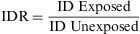
In recent years, odds ratios (ORs) have been widely utilised in reports and in biomedical scientific literature. Their popularity is derived from the fact that this measure provides a good estimator (together with the corresponding confidence intervals) of the relation between two binary variables and enables the user to apply logistic regression to examine the effects of other variables on this relation.6 The OR, also known as the Cross Product Ratio, is the ratio between two odds, and is frequently calculated in case-control studies, although it may be used in any type of epidemiologic design. It is calculated as follows:
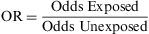
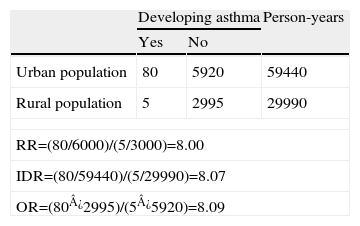
Its value cannot be less than zero, but it has no upper limit; i.e. its range is zero to infinity. When the disease occurs infrequently, the OR provides values similar to those of the RR, although the OR will always tend to overestimate the magnitude of the association between the risk factor and the outcome.Example 5 Cohort study to evaluate the development of asthma among adult non-smokers aged 20–60 years, comparing a group of residents in large cities (population of over 500,000) and those in rural areas (towns and villages with less than 5,000 inhabitants), with a follow-up period of 10 years. See Table 2.
The standardised mortality ratio (SMR) is a variant of the relative risk, which compares the mortality observed among a given population group with respect to the mortality that would be expected if the rates of specific mortality by age groups were the same as those for a standard population, and this measure can then be used in the indirect adjustment of rates. The SMR can be expressed as a ratio or as a percentage.
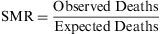
The result describes how many more deaths (as a multiple) are observed within a population, in comparison with the predicted value. An SMR ratio of 1 (or a value of 100%) means there are no differences in mortality between the sample population and the expected value among a standard population.
Measures of potential impactIn all measures of impact, it is assumed that the association between exposure and disease occurrence has previously been shown to be causal. Measures of potential impact estimate the disease load attributable to a given factor, and forecast the benefit to be derived from a public health action taken to minimise or eliminate the effects of exposure.7
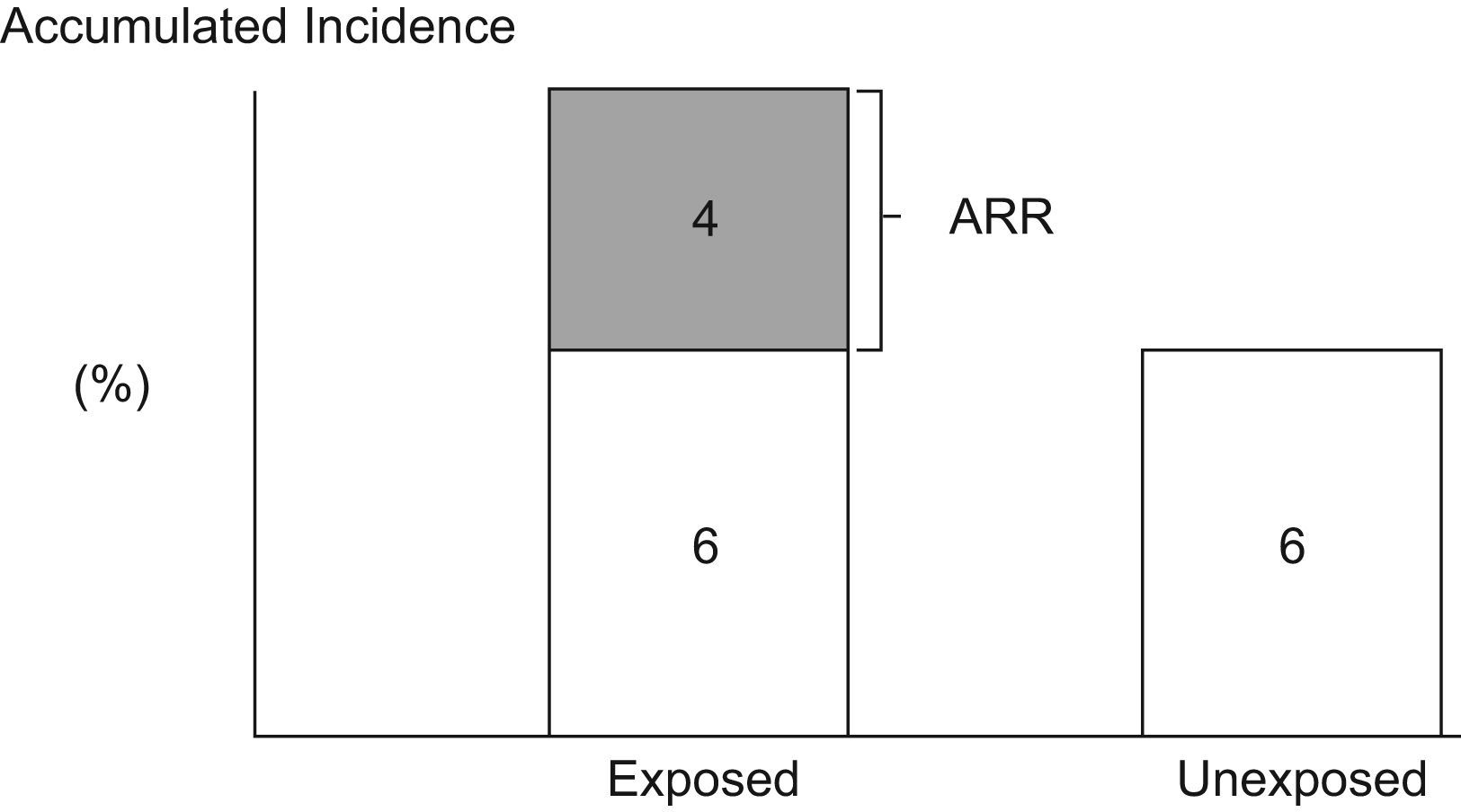
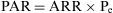
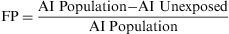
Attributable RiskAttributable Risk (AR) or Absolute Risk Reduction (ARR) is the proportion of the incidence of a disease among the exposed population that is due to the exposure. It is the incidence of a disease in the exposed population that would be eliminated if exposure were eliminated. In a cohort study, ARR is calculated as the difference in cumulative incidences (risk difference) or incidence densities (rate difference). Fig. 1 shows an example for accumulated incidence.


In case-control studies, if the disease is a rare event (less than 10%), although neither the incidence nor the attributable risk can be calculated directly, they may be determined indirectly when, by means of another source of information, the total incidence has been determined (by summing the exposed and the unexposed populations).
The Population Attributable Risk (PAR), also known as the Population Risk Excess, is the proportion of the incidence of a disease in the population (exposed and unexposed) that is due to exposure. It is the incidence of a disease in the population that would be eliminated if exposure were eliminated.

When the accumulated incidence among the unexposed population is not known, the PAR cannot be calculated directly using the above expression, and so the following must be applied:
In which Pe is the proportion of exposed persons within the population. In a cohort study, we can estimate Pe from the sample, as it is assumed that the proportion of exposed subjects in the sample is the same as that in the population as a whole. In a population-based case-control study, Pe would be estimated from the proportion of controls exposed.5
Attributable FractionThe Attributable Fraction or Attributable Proportion is, for a causal association, the proportion of the caseload that can be attributed to a particular exposure. It is the causal attributable difference divided by the incidence rate in the group.1 It quantifies the proportion by which the rate of incidence would be reduced if the exposure in question were eliminated. When the Attributable Fraction is applied to exposed individuals, it is termed the Attributable Fraction Exposed (AFe), and when applied to the whole population, it is known as Attributable Fraction Population (AFP).
The Attributable Fraction Exposed or Attributable Risk Proportion (ARP) is obtained by dividing the absolute effect by the incidence among the exposed group. Thus:

The OR as an estimator of Relative Risk is calculated using the following formula:

The Attributable Fraction Exposed is an important measure in the field of public health, used to evaluate priorities in healthcare treatments.
The Attributable Fraction Population or Population Attributable Risk Fraction (PARF) is the proportion of the disease or specific health problem among the population that is attributable to the exposure and which would be prevented if this exposure were eliminated. In the absence of variables that might generate bias or confound the causal relation between exposure and effect, the PARF or AFP can be estimated using the following formula:
An equivalent formula for a cohort study would be:
where Pe is the proportion of exposed subjects among the population. The RR can be estimated from the OR.Number Needed to Treat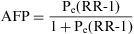
The Number Needed to Treat (NNT) is a popular index that is used to describe the results of randomised trials and other types of clinical study. It states the number of persons who should be given a particular treatment or preventive measure, with respect to the standard treatment, in order to prevent a case of disease, or the undesired outcome. This measure can be obtained for trials that report a binary outcome.8

The closer the NNT values are to 1, the more effective the treatment or intervention is, as the latter is applied to a smaller population in order to prevent the undesired outcome.
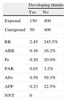
When an intervention produces an adverse event, its impact is measured by the Number Necessary to Harm (NNH). This is calculated using the same formula as for NNT, but the valuation made is the opposite, i.e. the greater the NNH, the better the treatment applied is, since it must be applied to a larger population before an adverse event or side effect appears.5Example 6 Cohort study to evaluate the development of allergic rhinitis (ARh) in children aged 46 years, comparing cohorts of children with smoker and non-smoker parents, during a one-year observation period. Table 3 shows a Cohort study of the development of rhinitis, and impact measures.
Interpretation: Allergic rhinitis is 2.45 times (or, in percentage terms, 245%) more frequent among children whose parents smoke than among those with non-smoker parents. The frequency of ARh among exposed children, attributable to exposure (i.e. the presence of smoker parents) is 16.2%. In 59.3% of cases of ARh among children exposed to smoker parents, the illness could have been avoided by elimination of the exposure (i.e. the parents giving up smoking). The frequency of ARH among all children that is attributable to the presence of smoker parents is 3.2%. 22.5% of all cases of ARH among children are due to exposure to smoker parents. For every six children whose parents stop smoking, one case of ARH would be avoided.
SoftwareA considerable amount of free software exists for the calculation of epidemiologic measures of frequency, association and impact. These programs include Open-Epi,9 Epidat,10 EpiData Software,11 and Epi Info,12 the latter being a public-domain program designed by the Atlanta Centre for Disease Control (CDC) that is particularly useful for public health studies. There are also numerous online calculators, especially those aimed at NNT and NNH calculations.
Final remarksMeasures of frequency, association and impact are the main statistical resources employed in epidemiology to describe the distribution of healthcare problems, establishing a causal relationship between exposure and disease, enabling users to evaluate the impact of preventive measures in the field of public health, among other areas of activity. For the correct use of these indicators, it is essential to distinguish between the diverse epidemiologic designs applied, because their characteristics determine the choice of the measure to be applied and the dimension of its interpretation.
We thank Glenn Harding for the professional translation of the paper. Francisco Rivas Ruiz is a research technician with a contract supported by Instituto de Salud Carlos III.
