


Any form of data analysis requires the prior creation of a database to house the study information collected in one format or other (questionnaire, clinical history, etc.). The design of such databases should be optimised to allow adequate statistical analysis without the drawing of wrong conclusions. In addition, prior to analysis, debugging or filtering of the variables is required in order to avoid doubling the effort made in extracting the results. The present study offers a series of suggestions for database design and debugging, to ensure that the later statistical analyses are based on the revised data.
Prior to any type of investigation, a study protocol must be established, contemplating methodological and technical aspects which will be applied in the course of the study. To this effect, it is very important to establish an epidemiological design adapted to the planned study objectives, and to adopt a rigorous and explicit methodology.
It is advisable for the protocol to include a case report form to be used in the measurement and collection of the information from clinical or case histories, or by means of some other kind of procedure. The case report form should specify each and every one of the fields which the investigator considers necessary for the study, with specifications where possible of the coding system used in each case.
Once the information corresponding to the case sample or series specified in the protocol has been obtained, computer-based data input is required1. Good data input is a decisive element for ensuring that the subsequent analyses are correct. It is common practice to design databases in which the variables have not been well defined, or where the information has not been entered with uniform or homogeneous criteria. This results in the need for later restructuring of the data files, with the associated waste of time and resources.
The present study aims to offer investigators the guidelines needed to design databases for any type of study, and explains the procedure required to filter or debug the information prior to the final statistical analysis2.
Designing a databaseIn designing a database, it is very important for investigators to select software with which they are familiarized. The section below describes some of the software applications that can be used.
In general, the data are entered in a box format obtained by crossing rows and columns. Each study variable conforms an individual column or field in the database, and all the data of a given subject are contained in one same row. Thus, if patient age is the first variable, gender the second variable, and marital status the third variable, the values of these three variables corresponding to a given individual will be contained in individual boxes aligned in a single row.
A series of recommendations for efficient designing of a database are provided below. The present study only addresses non-relational databases, i.e., those in which the data are contained in a single table or file. In comparison, relational databases comprise complex structures3 in which different data tables are related though key fields.
Data file structureThe first step is to clearly establish the variables to be included in the file, in order to define the data fields according to the type of variable involved.
- 1.
Quantitative variables (i.e., those measuring amounts) are to receive an adequate numerical format, indicating whether they correspond to integers (without decimals) or real numbers (with decimals). Whenever possible, these variables should be entered in numerical form, not grouped into intervals, since the latter approach gives rise to information losses.
- 2.
Qualitative variables (i.e., those measuring categories) are generally coded to allow faster and more homogeneous processing. As an example, in relation to subject marital status, it is general practice to code the different categories as follows: 1 = single, 2 = married / partner, 3 = separated/divorced, and 4 = widowed. In this context, it is always easier to enter number codes than category labels, since the latter approach entails a risk of error (e.g., entering uppercase or capital letters in one case and lowercase in another). In most statistical programs it is possible to define these category labels a posteriori, and it is convenient to keep them at hand in order to identify the different categories.
For variables of this kind it is advisable to generate a coding manual with the codes corresponding to all the categories, so that each time the database is used a document is available to identify the content of each variable and the way in which it is measured (i.e., independent of the person creating the database). This document is usually included in the established study protocol, in the section corresponding to measurement variables, or as an annex identifying the case report form.
When qualitative variables contain many categories, it is sometimes preferable to enter the data as chains, followed by grouping and coding – although this may be time consuming. Emphasis is placed on the convenience of entering the data in coded form, as described above.
- 3.
Data relating to dates are to be defined as such in the database, in short format (day/month/year, dd/mm/yy). Data collected as hours and minutes should be transformed to decimal format for analytical purposes, dividing the minutes by 60 and adding them to the recorded hours.
- 4.
Dichotomic variables (with only 2 possible values) should be coded as 0 and 1 (where 0 = absence and 1 = presence). In the case of the variable sex or gender, 0 and 1 should be taken to indicate females and males, respectively. In general, such coding will depend on the established objective. Thus, if the aim is to determine risk factors, 1 (or the highest number code) should be used in reference to the category favouring appearance of the event of interest.
- 5.
Those variables that allow multiple and non-mutually excluding responses are to be defined as different fields (one for each variable). As an example, when considering a series of symptoms classified as pruritus, rhinitis, asthma and others, one variable is defined for each symptom – followed by input as 0 if the subject does not have the symptom in question, or as 1 if the subject has the symptom. It is very common to find databases in which all these data have been entered under one same variable – thereby making analysis impossible. As an example, if a subject presents pruritus (coded as 1) and asthma (coded as 3), it is common to find both variables merged into one as “1,3” – when in fact the value 1 should be entered in the column corresponding to pruritus, with the value 1 in the column asthma, and values of 0 in the columns rhinitis and others, since the subject in question does not have these latter symptoms.
- 6.
When repeated measurements of one same subject are made, they should be reported as independent variables. As an example, different spirometric measurements over time are to be entered as different variables (one for each measurement made).
- 7.
Missing values (i.e., values not obtained, lost values, data collecting errors, etc.) are to be coded in blank or using a code outside the range for the variable in question – with later indication in the program of the value represented by the mentioned lost code, in order to prevent such data from being included in posterior analyses. Whenever possible, it is advisable to use the same scheme for the coding of these values, for all variables. As an example, if the parameter age has not been obtained for some patients, these values are usually left blank, or alternatively the value “–9” is entered – the program later indicates that this code represents a missing value (subject age cannot yield the value “–9”).
- 8.
All databases tend to contain an identification variable at the start. Such an identification code must be unique for each subject, guaranteeing data confidentiality, and making it possible to link each case to the questionnaire, clinical history or information of interest for the study.
In general, the data are entered by rows, each row corresponding to an observed case or subject. In some databases and spreadsheets, as well as in most statistical packages, drop-down menu fields can be used for qualitative data input – a fact that facilitates input processing.
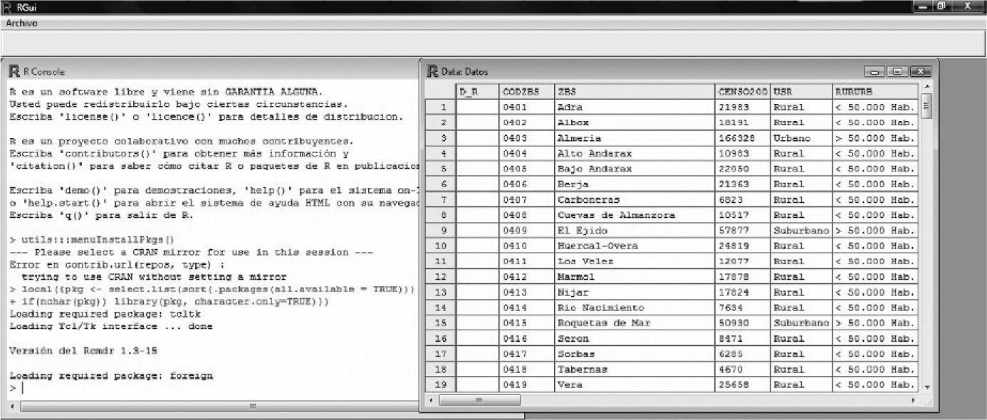
Data input or entry is sometimes an arduous and time-consuming task, but it must be done very carefully, since the success of the study is largely dependent upon correct data input. In order to accelerate this process, it is advisable to become familiarized with the keyboard shortcuts of each software application, and use of the tabulator. If allowed by the application, the use of data input forms is an interesting option. Figure 1 offers an example of a database defined by the R freeware application.
Debugging the database
After designing the database, the data must be pre-processed or debugged4 in order to detect possible anomalies secondary to the typing process, or because they correspond to extreme observations. It is estimated that 3–5 % of all data are entered erroneously5 – a figure that may reach 27 %6 in the case of double input data (i.e., data entered by two independent investigators).
In general, recoding of the variables is always required after data input and debugging7. Doing this before the quality control step would imply the risk of having to repeat the calculation of the new variables with the revised data. It is advisable to keep a copy of the original database, and then perform the necessary modifications.
Recoding involves the creation of new qualitative variables from other qualitative or quantitative variables found in the data file, to allow categorization in the form of intervals. In all cases recoding is performed after entering the data – not at the time of data collection (unless where necessary), since information would be lost as a result. As an example, if we question subjects about their age, it is always preferable to collect the datum as a number, not as an interval – except when in certain populations the latter is considered sufficient to identify the individual, or when it is not possible to collect the parameter in its original format.
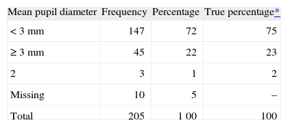
Qualitative variablesQualitative variables are debugged or filtered by preparing frequency tables. A frequency table offers a summarised presentation of the different categories of a given variable along with its corresponding frequencies (number of cases contained in each category) and percentages (number of cases of each category multiplied by 100 and divided by the total number of available cases). In preparing these tables it must be confirmed that there are no categories different from those actually measured. As an example, the variable gender must have only two categories. Any appearing third category (other than that serving to identify missing values) will constitute an error.
Table I shows a frequency table containing three values entered in the database with code 2 (not valid for this variable); these three values therefore must be checked in the database to determine whether they correspond to 0, 1, or missing values. Recalculation of the table is then required.
Frequency table for qualitative variable debugging of filtering
| Mean pupil diameter | Frequency | Percentage | True percentage* |
| < 3 mm | 147 | 72 | 75 |
| ≥ 3 mm | 45 | 22 | 23 |
| 2 | 3 | 1 | 2 |
| Missing | 10 | 5 | – |
| Total | 205 | 1 00 | 100 |
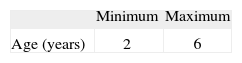
Quantitative variables are debugged by calculating the minimum and maximum values, making sure that they fall within the possible range of values for the variable in question. For example, in conducting a study on the prevalence of Parietaria allergy in nursery school children, the variable age may range from 3–5 when measuring age in years (36–60 if measured in months), but the minimum value must not fall below 3 years and the maximum value (upper limit of the range) cannot exceed 5 years (or the equivalent values in months).
In Table II it can be seen that there are values which do not comply with the nursery school age range (2 and 6 years of age). It is not possible to determine how many incorrect values there are, unless a frequency table is created to identify them.
In debugging or filtering a numerical value calculated as the difference between two dates, the values must always be positive. Any negative values must be revised. As an example, the calculated delay in days between the diagnosis of allergy and its treatment must be equal to or greater than zero in all cases.
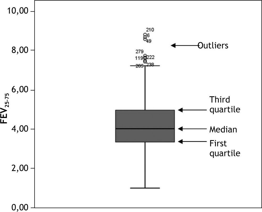
It is also advisable to represent quantitative variables by means of a boxplot, which is very indicative in the case of anomalous or out of range observations. For data ordered from lesser to higher values, a boxplot graphically corresponds to a vertical box where the lower end represents the first quartile (i.e., the value below which 25 % of the sample is found), the upper end is the third quartile (the value below which 75 % of the sample is found, or above which 25 % of the sample is located), and the median is found within the box (the value above which 50 % of the sample is found, and below which 50 % of the sample is located). External to the box at both its upper and lower ends we have two lines calculated from the two most extreme values or observations of the sample. Those observations identified outside these two external lines (both above and below the box) are outlier observations which must be revised, since they may be due to a typing or processing error. An example of a boxplot is found in Figure 2.
Software for designing and/or analysing databases
Many programs for developing databases can be found on the market. The following software tools are used:
- –
Spreadsheets: These allow us to construct databases with rows for the cases and columns for the variables. The first (or heading) row should be used to define the names of the variables. Spreadsheets offer the advantage of calculating the new variables as the data are entered. They can be used to perform descriptive studies and some analyses of the relationships between pairs of variables. (examples: Excel, StarOffice Calc., etc.).
- –
Databases: These are able to store large sets of inter-related data. The fields are defined as inter-related table structures, and forms can be established to facilitate data input. Databases are very useful for descriptive statistical studies, but are less apt for more complex analyses. (examples: Access, StarOffice Base, etc.).
- –
Text format: When no software is available for data input, a text or universal format can always be used, in which the data are generally entered in the form of columns, separated by a tabulator. The advantage is that any program can import files of this kind, and they can be defined from any computer system. The drawback of the text format is that data entry can prove tedious. These programs do not allow any kind of data analysis. (examples: note blocks, etc.).
- –
Statistical packages: In general, all statistical packages contain a spreadsheet for data input and recoding. They have the advantage of being able to store the files in the corresponding statistical software format for later analyses – though conversion is required when importing from or exporting to other types of programs. (examples: SPSS, Stata, Statgraphics, etc.).
The use of word processors for data input in table form is not advised (examples: Word, StarOffice Writer, etc.), since the above mentioned software applications do not accept such a format, and “copy” and “paste” processing may fail to preserve the originally defined format of the study variables.
It must be taken into account that, although a database can be designed from any database application software, spreadsheet or statistical package, only the latter is able to afford a complete statistical analysis of the included data. In general, database application software allows descriptive calculations to be made, while spreadsheets are able to perform certain comparative analyses between pairs of variables (e.g., Student t-test, Pearson correlation coefficient)
- –
but we must resort to statistical packages when more complex statistical studies are required.
Thus, while a database can be designed using any of the aforementioned programs, it is advisable to import the data to a statistical package for the debugging or filtering process, since the boxplots are created automatically with such packages, while boxplot construction is manual in the case of spreadsheets.
There are many websites where the different statistical packages available on the market can be consulted. The following are among the two most representative sites:
http://en.wikipedia.org/wiki7List_of_statistical_packages
The current tendency is to use freeware for database design and analysis: Openoffice (similar to Microsoft Office), Epidat (for tabulated data), R, PSPP, etc. All these programs are free and can be downloaded from the Internet.
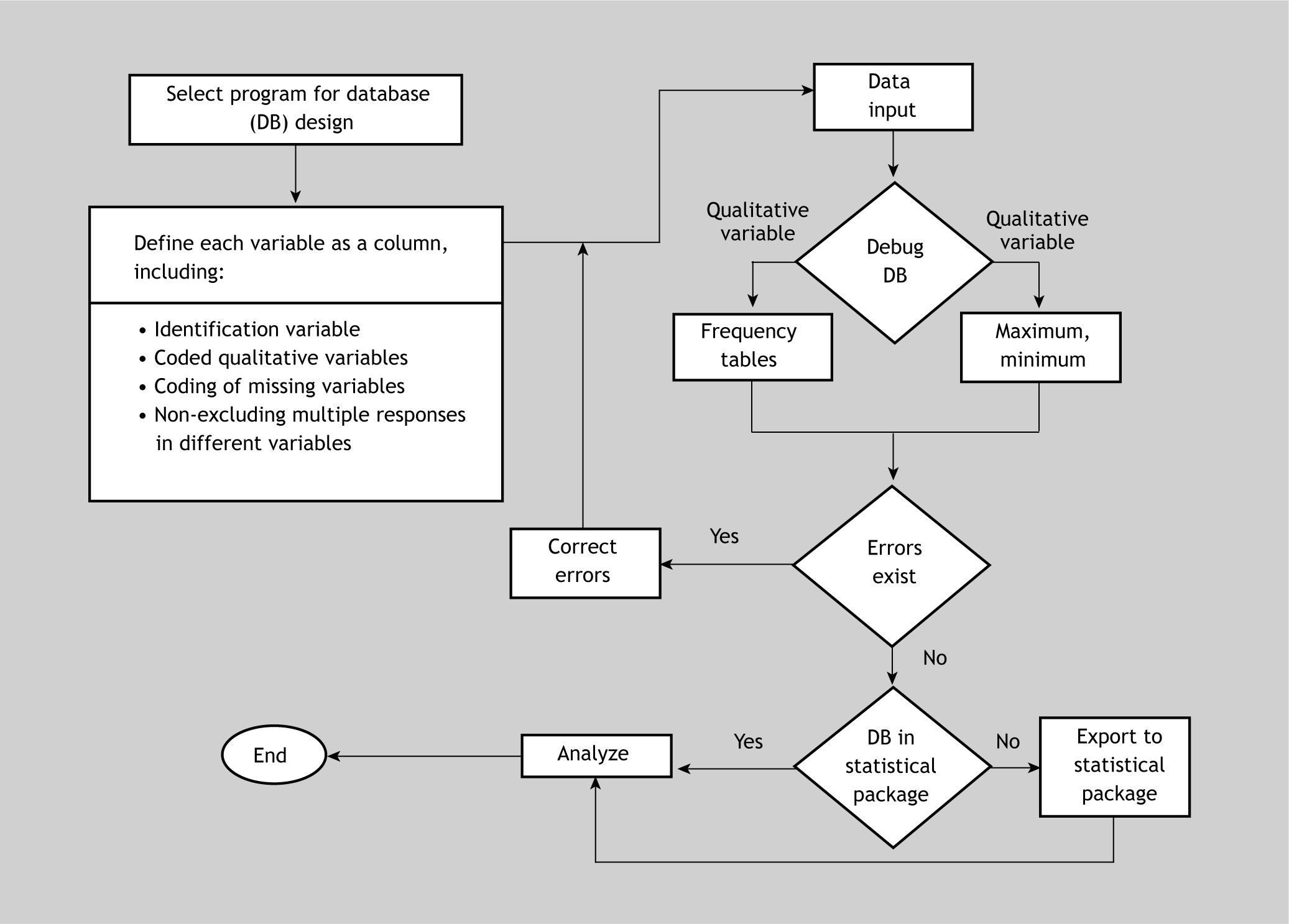
Algorithm for data file creation and debuggingFigure 3 shows a summarised algorithm with the general steps needed to design and debug or filter a database for subsequent analytical purposes. The debugging phase can be carried out before or after importing the data to the statistical package. On the other hand, the recoding phase has not been included, since it must be carried out once the data set has been debugged – regardless of whether this is done using the original program with which the file was created, or using the statistical package after importing the data.
Final considerations
It is advisable to create a backup copy and keep the database in a safe place before analysis, once initial data input has been completed, and debugging has been carried out.
Databases should be created in abidance with the requirements of Organic Law 15/1999 of December 13 relating to Personal Data Protection 8 (applicable law in Spain).
Conflict of interestThe authors have no conflict of interest to declare.
