


The data provided by clinical trials are often expressed in terms of survival. The analysis of survival comprises a series of statistical analytical techniques in which the measurements analysed represent the time elapsed between a given exposure and the outcome of a certain event. Despite the name of these techniques, the outcome in question does not necessarily have to be either survival or death, and may be healing versus no healing, relief versus pain, complication versus no complication, relapse versus no relapse, etc.
The present article describes the analysis of survival from both a descriptive perspective, based on the Kaplan–Meier estimation method, and in terms of bivariate comparisons using the log-rank statistic. Likewise, a description is provided of the Cox regression models for the study of risk factors or covariables associated to the probability of survival. These models are defined in both simple and multiple forms, and a description is provided of how they are calculated and how the postulates for application are checked – accompanied by illustrating examples with the shareware application R.
In some medical investigations it is common to find a group of patients who enter the study as they are recruited, and in which the outcome variable is the time of occurrence of a given event: death, healing, the presence of adverse effects, relapse, etc. In studies of this kind questions are raised such as the probability or percentage of patients who survive after a given time, or whether the survival times are similar between treated and untreated patients, among other aspects. In these cases, the observations are referred to as survival data or simply analysis of survival, with the objective of determining the probability of survival up until the end of a given follow-up period.1
The analysis of real survival would be determined by occurrence of the terminal event in all the patients, but since their complete follow-up is not possible, evaluation is made of survival up to a given instant or timepoint. In investigations of this kind, the patients who are recruited close to the end of the study contribute a shorter follow-up period than those who enter the study at the start. The duration of follow-up can vary according to the investigation being carried out. Thus, survival in an experimental study in rats may be evaluated in days, while relapse or death in cancer patients usually involves months or even years.
At the end of the follow-up period, which is usually predetermined by the investigator, the following situations may apply:
- -
The patient enters the study, and at the end of follow-up the terminal event has not occurred. In this case, the time of survival is said to be censored, or the patients are censored, in the sense that the full period of observation has ended before the event occurs – although it is not clearly known whether the mentioned event will occur or not.
- -
The patient enters the study and is subsequently lost after a given follow-up period (change in address, dropout, death due to some cause other than the evaluated cause, traffic accident, etc.). These would also represent censored cases, since survival time is registered up until the time of patient loss.
- -
The patient dies within the follow-up period, independently of the time of entry to the study. These are non-censored cases.
In the analysis of survival, two variables are therefore necessary: a first variable represented by survival time until the event occurs (difference between the date of the end of the study and the date of inclusion in the trial – the latter being the date of treatment, diagnosis, or any other date), and a second variable indicating whether the case is censored or not. The latter variable is usually represented as 0=censored, 1=non-censored, or equivalently 0=not died, 1=died; 0=no relapse, 1=relapse, etc.
An important assumption to be taken into account in studies of survival is the fact that the prognosis of patient survival must remain constant over the course of follow-up, and that the patients who are lost likewise have the same prognosis as those who remain alive.2
Kaplan–Meier methodThe following example is provided in order to orientate the reader. Suppose we wish to compare the survival times between two groups of patients (cases and controls) after a certain duration of follow-up, a first idea would be to consider the comparison of survival between the two groups applying the Student t-test or the equivalent Mann–Whitney (Wilcoxon) non-parametric test.3 This is not possible, for a number of reasons. The first reason is that some subjects are censored and have been analysed only during the time for which the study lasts, while on the other hand, the patients are entered in the study progressively, i.e., not all subjects have the same duration of follow-up.
In turn, on summarising the survival results, the calculation of mean values does not make much sense, since it is a very asymmetrical measure; it would therefore be more correct in these cases to calculate the median or even the mode. Furthermore, over each time segment, previous survival on the part of the patient must be taken into account.
For these reasons we use specific techniques for estimating survival. Of these methods, the following are the three most widely used options4:
- -
Direct method. This is the simplest method. Calculation is made of the percentage or probability of patients still alive at the end of a given time interval, including only those patients exposed to fatality in that period. This method poses the inconvenience of not taking into account the live losses up until the evaluated instant or timepoint.
- -
Actuarial method. This technique is more commonly used when populations are analysed. Calculation is made of probability dividing the period of follow-up into segments of fixed length, considering that those who have died have been exposed for half of the interval. This technique therefore offers approximate probabilities.
- -
Kaplan–Meier method. This technique is more commonly applied to samples, particularly of small size,4 although it can also be applied to larger samples. It is similar to the previous method, with the difference that the time is not divided into periods of fixed length but of variable duration. Each period or segment is the interval between two non-simultaneous terminal events. In addition, in each segment, calculation is made of the probability of survival as the product of the probability of survival at the start of the interval and the probability of survival at the end of the interval – since the subject was alive at the start (conditioned probability of death in the interval, since the subject reaches it alive).5 This method is more precise than the previous technique, since it affords exact probabilities.
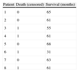
Table 1 represents the survival times in eight patients with breast cancer followed-up on for a period of eight years. The variable exitus (death) is the outcome in this case, and each patient contributes a given time within the study. Fig. 1 graphically displays these survival times, where it is seen that each subject has been progressively entered in the study with the corresponding end result. The non-censored or deceased patients are subjects 3, 4, 6 and 8 (in red), and the censored patients (in blue) are cases 1, 2, 5 and 7. Note that cases 1 and 7 were lost before the conclusion of the study, while cases 2 and 5 were still alive at the end of the study.

Graphic representation of the survival times corresponding to the patients in Table 1.
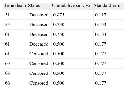
The distribution of probabilities constructed with any of the three methods described above, together with the intervals in which the probabilities are calculated, conform the so-called survival table, in which specification is made of at least the time in which some event occurs (censored or otherwise), the probability of survival in that interval or the cumulative probability up to that interval, and estimation of the standard error. The contents of the columns in this table may depend on the statistical program used for the calculation. The interpretation of the cumulative probability in the k interval would be the percentage or probability that a given patient survives within the k interval, knowing that he or she has survived in the k−1 interval.
Table 2 shows the estimations of survival corresponding to the data in Table 1, according to the Kaplan–Meier method. Initially the times are ordered from shorter to longer. In the first time instant a patient dies, as a result of which the probability of survival in interval 31–55 would be seven patients among the eight at risk at the start, i.e., 0.875. For the second interval, the probability of survival would be 6/7 (six remain alive among seven patients at risk), multiplied by the probability of the previous instant, i.e., 0.750. We in turn would continue in this way until the table is completed.
Kaplan–Meier survival table for the data in Table 1.
| Time death | Status | Cumulative survival | Standard error |
| 31 | Deceased | 0.875 | 0.117 |
| 55 | Deceased | 0.750 | 0.153 |
| 61 | Deceased | 0.750 | 0.153 |
| 61 | Deceased | 0.500 | 0.177 |
| 61 | Censored | 0.500 | 0.177 |
| 63 | Censored | 0.500 | 0.177 |
| 65 | Censored | 0.500 | 0.177 |
| 68 | Censored | 0.500 | 0.177 |
Once the probabilities have been calculated in each segment, they are usually accompanied by expression of the standard error, which allows us to construct confidence intervals for survival through approximation to a normal distribution (survival±1.96×standard error).
If axis x is used to graphically plot survival time and axis y is used to plot cumulative survival, we obtain the survival curve, which usually begins at one and gradually decreases as the subjects die – generating a step in each case.6 If several patients die in the same interval of time, only a single down step is produced, though of greater magnitude (cases 4 and 8 in Table 1). The survival curves are usually accompanied by their respective confidence intervals. These curves only represent the survival time of the patients in the study, showing no variability in survival times between patients, reflected through dot plots and scatter plots.7
The survival tables and curves are next applied to an example with a larger number of cases, carried out with the R program. We start from a sample of 1207 women with breast cancer who have been followed-up on during the 12 years of the study. We wish to estimate the survival time and analyse possible risk factors related to the cancer. The outcome variable is death due to this cancer.
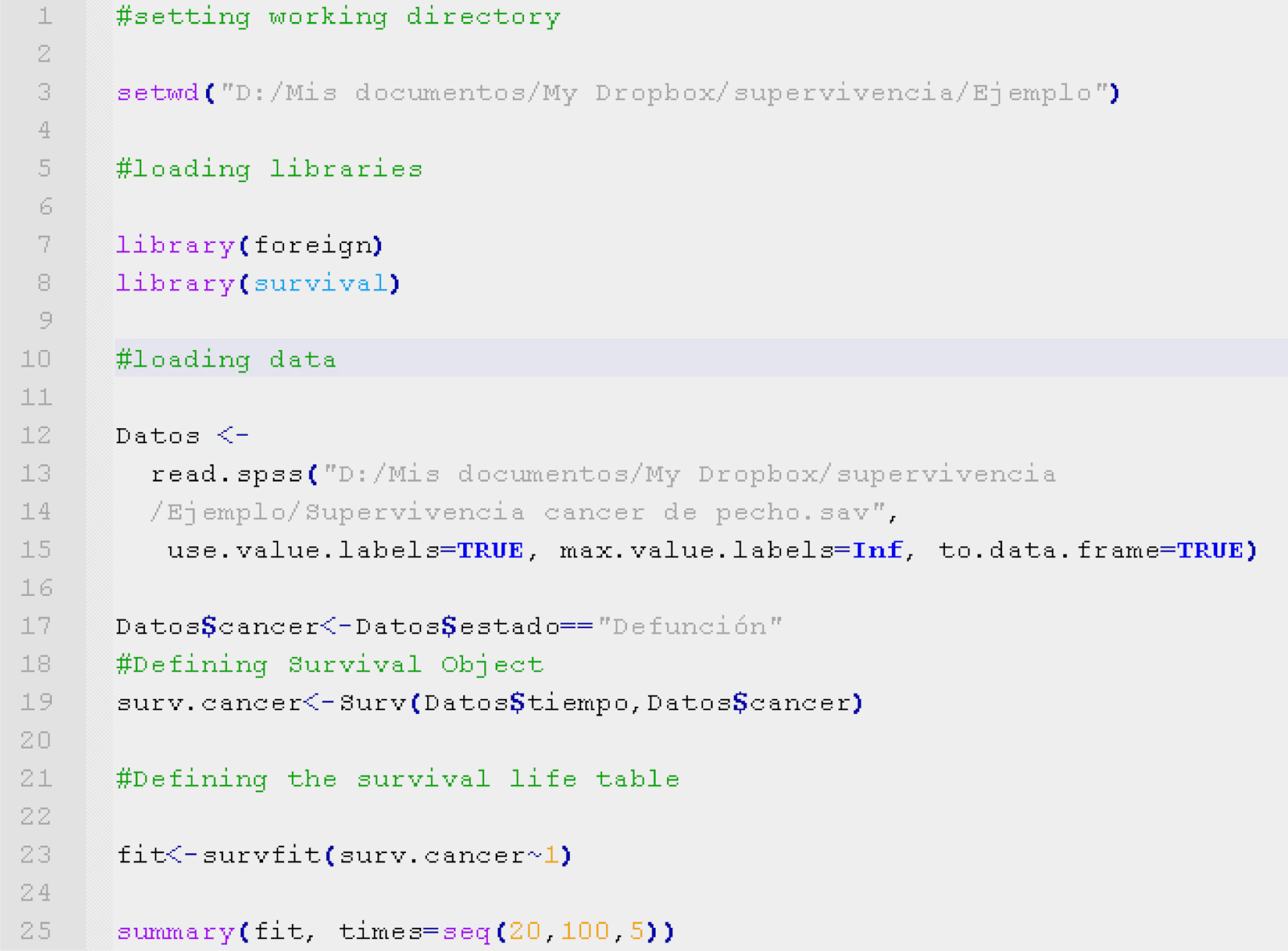
The code shown in Table 3, written with the R program language,8 allows loading of the data and construction of a survival type object. After loading the survival9 (for the manipulation of survival studies) and foreign libraries10 (for importing data from different statistical packages such as SPSS), we load the study data set from an SPSS database using the function read.spss.

This database is assigned with the name Data. The variable Data$cancer is a dichotomic variable that describes the presence or absence of the event under study (in this case death due to breast cancer). The survival time is the variable Data$time, expressed in months.
Once the variables survival and survival time have been registered, the object of survival is defined by the function:
as can be seen on line 19 of Table 1.
In order to calculate the life or survival table, we construct the Kaplan–Meier model by means of the function survfit, fitting the survival object with the formula (Surv∼1) (line 23), and presenting the table by means of summary of the model.
The result obtained is a table with the following information (Fig. 2): survival time (grouped 5 by 5 starting from 20 to 100 months), number of women at risk in each interval, number of events (deaths due to breast cancer), cumulative survival estimated with the Kaplan–Meier method, standard error and confidence interval associated to each interval.

In this way it is possible to know, for example, that the probability of surviving at least 60 months is 0.918, this probability being located within the population range (0.898 and 0.940), with a confidence of 95%. The same considerations apply to the readings for the other time values.
Based on this table it is simple to construct the survival curve associated to the Kaplan–Meier model, using the function plot (line 18 of Table 4) on the survival fit constructed in the previous section. If we wish to represent the survival curve together with the confidence intervals and event markers, we use the commands conf.int and mark.time (TRUE or FALSE for both); in the example this has been separated in order to illustrate the curve more clearly.
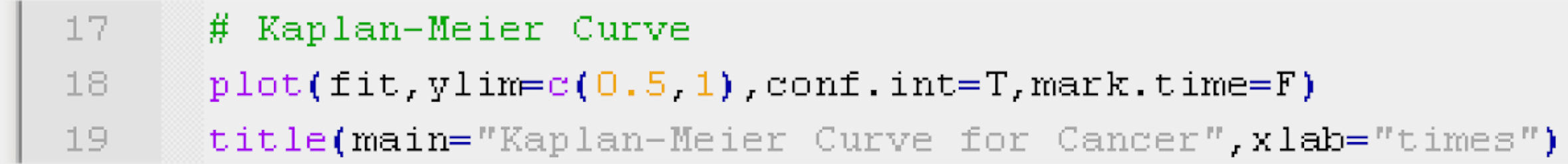
In order to adjust the values of the ordinates axis (y) to the values obtained, we can use the function ylim=c(y0, y1), employing the function title to include title and axis markers in the figure, line 19.
As a result of executing the code of Table 4, we obtain Fig. 3. Note that the survival value associated to an individual with a study period between 0 and 120 months does not drop below 0.8 (implying a low risk of death due to breast cancer, since the probability of survival for this type of cancer at the end of the study is over 80%).

The interpretation of the curve would be the same as for the survival table. Note that for greater survival times the intervals become longer, since the sample size gradually decreases as the follow-up period progresses.
Comparison of two or more survival curvesThus far we have seen how to generate a survival table and its plot, and how to interpret and read both of them. In summary, we have described the probability of survival of a concrete event. The investigator now raises another series of questions: Is the probability of surviving the study event greater according to whether or not the patient presents a possible risk factor? or in other words, Do more patients without the factor survive the event than patients with the factor?
What we have seen in the preceding section is not enough to answer this question; we have to compare two or more survival curves and/or two or more survival tables – those of the patients with the risk factor versus the patients without the risk factor. This represents a contrast of hypotheses,3 and in this case the alternative hypothesis, or non-equality hypothesis, would be that the probability of surviving the event differs according to whether the patient presents the risk factor or not. Furthermore, according to the previously raised research question, there is evidence that the subjects without the factor show longer survival. Thus, the contrast would be:
where Sp is survival in the group with the risk factor (i.e., present) and Snp is survival in the group without the risk factor (i.e., not present).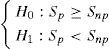
In order to carry out this contrast, we distinguish whether the comparison between curves is made between two groups (comparison of two curves for a dichotomic variable), more than two curves (categorical variable in general), or between several curves identified by a continuous-type variable (survival curves for several age segments).
For the comparison of two or more survival values we apply the log-rank statistic (the entered variables are the same as in the previous section, i.e., survival time and event, although now adding the comparison of survival according to a covariable, whether qualitative or quantitative).
This statistic is calculated based on determination of the observed number and the expected number of events for each survival time. To this effect we use the chi-squared statistic, adopting a significance value which for a 95% confidence level (significance under 0.05) would allow us to accept the alternative hypothesis that the presence of the risk factor in the patient lessens the probability of survival.
Dichotomic variablesContinuing with the example of survival in breast cancer, it would be interesting to determine whether the presence or absence of adenopathies influences patient survival. This independent variable (presence or absence of lymph node invasion) is dichotomic; as a result, two curves are compared and the probability of survival in each of them is examined. From the literature it is known that adenopathies reduce the probability of survival in breast cancer patients.
Applying the Log-rank test, the program displays are the same as in the descriptive Kaplan–Meier procedure, although in this case they are dual: one for the patients with adenopathies and another for the patients without adenopathies – establishing comparison between the two groups.
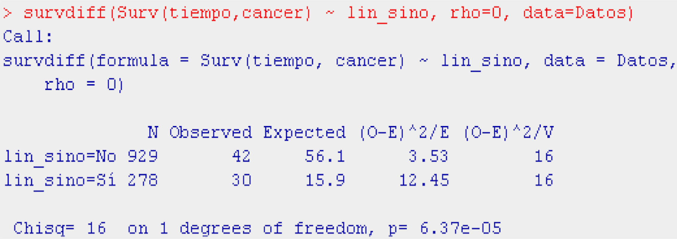
Continuing with the example in the R program, and using the function survdiff, we construct the log-rank test for comparison of the populations with and without adenopathies (Table 5).

The function survdiff takes as argument a survival model fitted for the factor of interest (Surv(time,cancer)∼factor), the dataset on which we are working, and a scale parameter (rho, equaling it to 0 yields the log-rank test) allowing us to modify the test for the case in which the distribution of events is rare.
The display generated by the program is a table with the number of individuals in each of the subpopulations, the number of observed and expected cases of death according to the null hypothesis, and the terms of the chi-squared statistic. Lastly, the results of applying the contrast of hypotheses (value of the contrast statistic, degrees of freedom (df), and p-value associated to the contrast) are presented.
The result of the test of hypotheses indicates that there are differences in survival between both groups (p<0.001); this information is completed with the survival curves, and the survival tables associated to each of the subpopulations (with and without adenopathies; Figs. 4 and 5).


Examination of Fig. 4 corroborates what was obtained on applying the log-rank test, i.e., there are differences in the survival curves between both groups, with lesser survival in the group presenting adenopathies. According to the table, for one same survival time, for example 70 months, the probability of survival in the absence of adenopathies is 92.6% (0.926), while in the group with adenopathies this probability decreases to 82.8%. Note that the confidence intervals of both curves only overlap after month 80, and prove parallel from that time onwards.
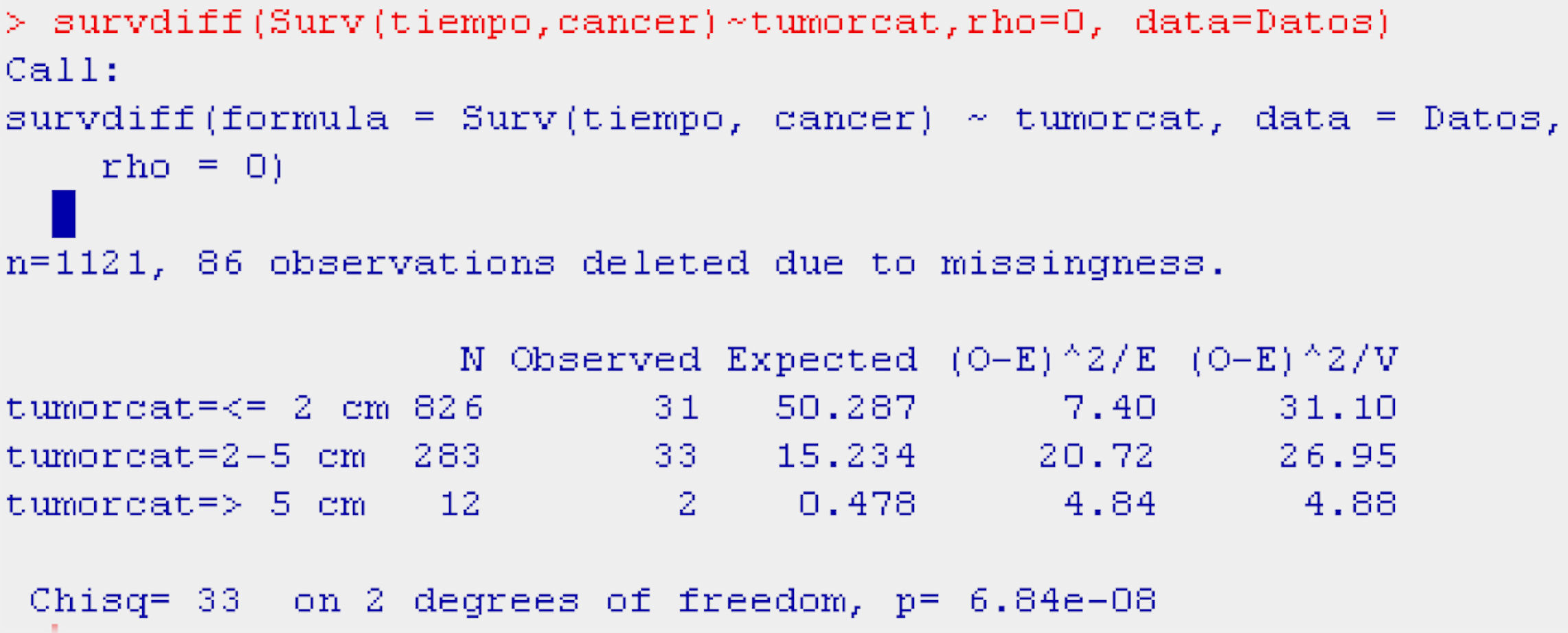
Categorical or polychotomic variablesIn the case of the independent variable having more than two categories, and continuing with the previous example, it would be interesting to analyse survival in breast cancer according to the size of the tumour, which may take the following values: ≤2cm/3–5cm/>5cm. It is assumed that the larger the tumour size the poorer the survival; thus, we obtain three survival tables and a plot with three curves – one for each category of the independent variable.
With the probability of survival shown by the tables in each of the categories, the reader can form an opinion of whether survival is longer or shorter according to the value of the independent variable. However, based on the log-rank statistic, we obtain the significance values – in this case a global value indicating possible differences or no differences between the probabilities of survival in each group, and posteriorly as many values as there are 2×2 combinations of the categories of the independent variable. In other words, we obtain a significance value for survival values in patients with a tumour size of ≤2cm versus patients with tumours measuring 3–5cm in size, and versus patients with tumours measuring >5cm.
Table 6 shows the example reflecting the above.

The display of the test (Table 6) likewise indicates that survival is better or worse in some groups versus the rest (p<0.001).
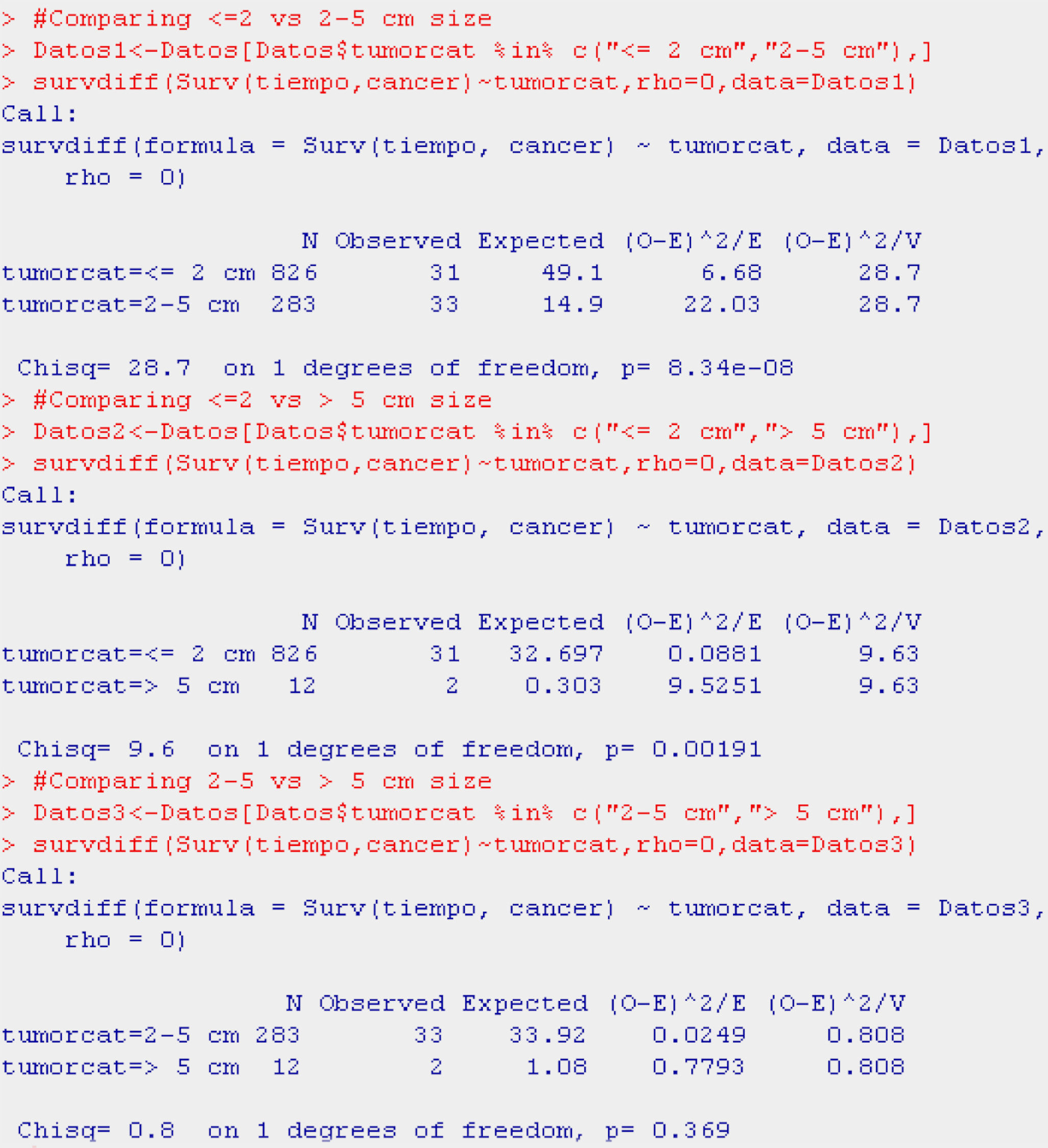
In the curve in Fig. 6 we see that the group with a tumour size of ≤2cm has greater survival than the group with tumour size 2–5cm, and that the latter group in turn shows greater survival than the group with a tumour size of 5cm or more. Likewise, the irregularity of this latter curve is due to the scant sample size in this particular group. On establishing 2×2 comparisons from Table 7, we see that the groups that differ with respect to each other are tumour size ≤2cm versus 2–5cm (p<0.001), and ≤2cm versus 5cm or larger (p<0.01). No differences in survival are observed between the two groups with the largest tumour size (Fig. 7).


Tumour size might be related to the presence or absence of adenopathies (interaction between both variables). This would make it necessary to segment or stratify the survival analysis for this variable of interest, i.e., survival according to tumour size for the patients with adenopathies and for the patients without adenopathies – yielding significance values for each group of patients, and per 2×2 combinations (Table 8).
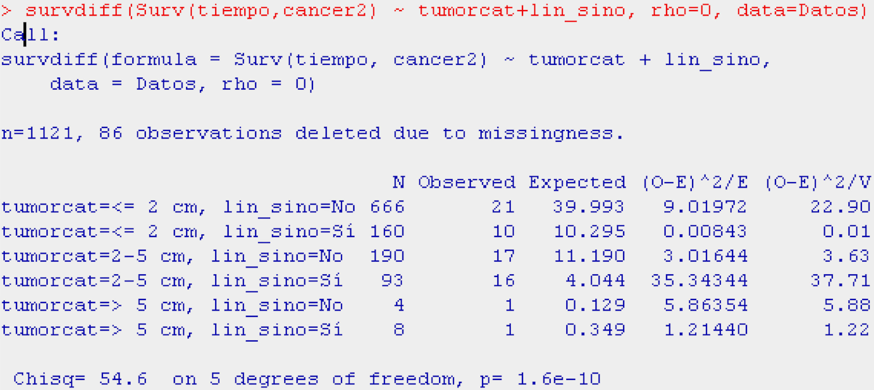
As can be seen in Table 8, both tumour size and the presence or absence of adenopathies are related to the probability of survival (p<0.001).
As the tumour size increases, and considering also the presence of adenopathies, the curves indicate that the probability of survival decreases. The inconvenience of stratifying the sample with more than one variable is that the sample size decreases considerably in each stratum. One way to avoid this situation will be seen in the following section with the application of Cox regression.
Numerical variablesWhen the independent variable analysed for changes in survival is of a numerical nature, the analyses and displays change. In this situation Cox regression is applied, as explained further below, and the survival values of the independent variable are replaced by relative risk (HR) values (in this case raw values) – their interpretation being similar to that of the Odds Ratio (OR) in logistic regression.11 In other words, it is shown how changes by one unit of the numerical variable exert a positive (risk factor) or negative (protective factor) influence upon the probability of patient survival.
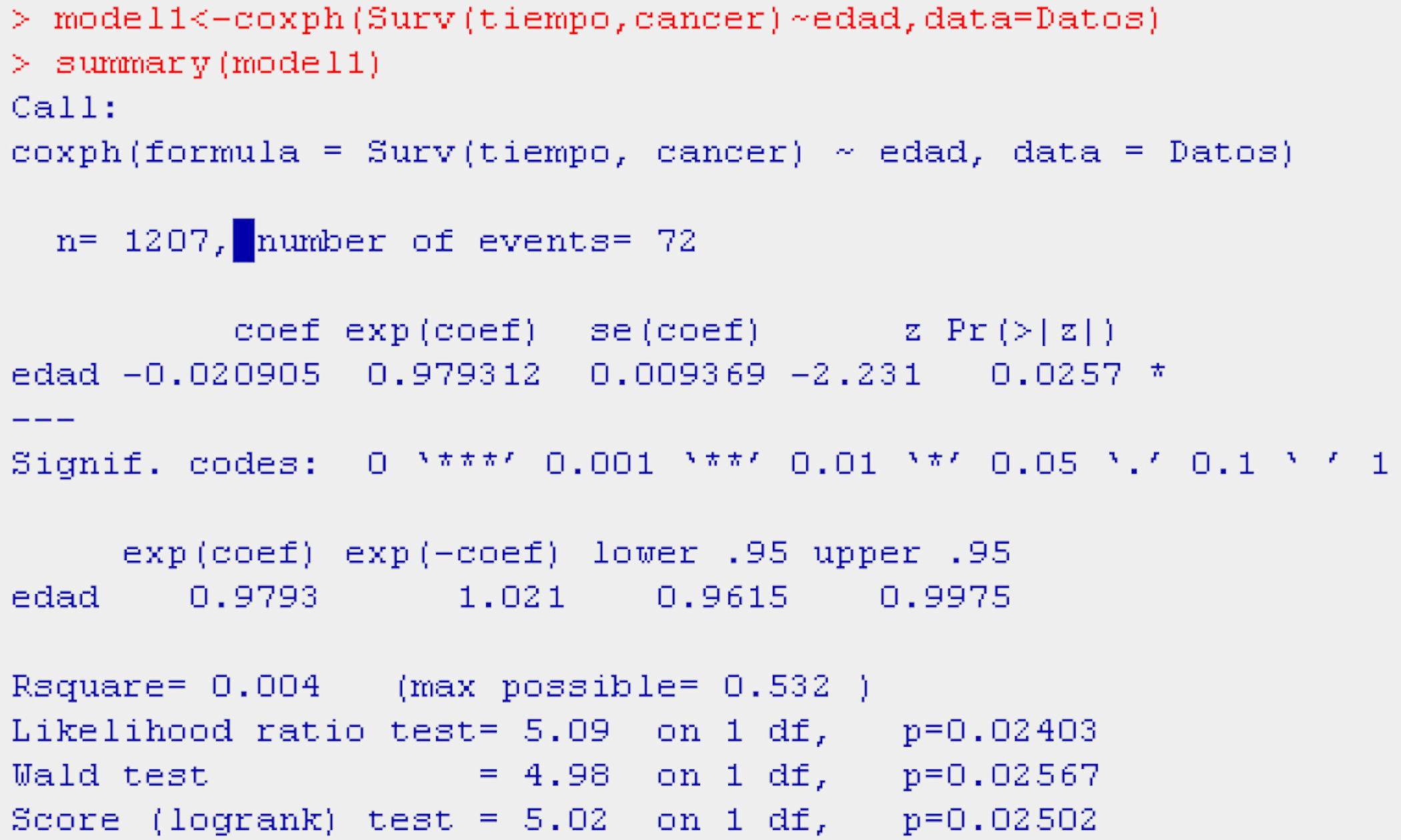
Continuing with breast cancer patients, we can see the way in which the variable age influences the probability of survival (Table 9).

As can be seen in the table, age is a protective factor (HR=0.9793) in relation to death due to breast cancer – the mortality risk decreasing by 2% for each year of increase in age.
Cox regressionIn relation to the previous example, examining the influence of patient age upon survival in breast cancer, an analysis of survival with the Kaplan–Meier method is not feasible, since the covariable is numerical, and we wish to determine how the probability of an event varies as the age of the patient increases by one year. If we were examining the influence of the variable upon survival based on this analysis, we would obtain tables and plots that are “impossible” to interpret due to the number of values which the covariable or risk factor can have.
Another option for using the Kaplan–Meier method would have been to establish age intervals, but this would have led to an important loss of information. This is the reason why regression analysis has been employed.
Considering that the dependent variable is dichotomic (presence or absence of the event), we could think of using logistic regression.11 However, we would forget another of the principal variables: the variable which measures the time from patient inclusion in the study to occurrence of the event or censoring. For this case, logistic regression is not adequate, and an alternative technique is used: Cox regression. Considering that age in the previous example is the only covariable in the model, simple regression was used; however, if we were interested in knowing the risk factors associated to survival in breast cancer, we would be dealing with multivariate regression – used to assess the effect of multiple prognostic variables upon the survival curve.
Such regression, as can be imagined, is similar to logistic regression, with the particularity that it studies the time to occurrence of the event fitting for a series of prognostic variables or factor, and that hazard ratio (HR) is the value returned by the model.
Cox regression equationThe equation of the Cox regression is as follows:
where Ln[h(t)/h0(t)] is the probability of survival at instant t, β0 the coefficient of the constant, and βi the coefficient for each covariable included in the model. The exponential of these coefficients is the hazard ratio (HR).The value of ¿ corresponds to the residuals of the model, in the same way as in the linear or logistic regression seen thus far in this series.11,12Conditions of the model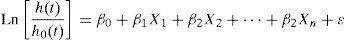
Further particularities of Cox regression are the type of variables that enter the equation:
- •
This model is based on the assumption of proportional risks, i.e., the risk between two subjects must remain constant over time (parallel survival curves that do not intersect).13,14 If this was not the case, then Cox regression would not be valid and other techniques would have to be used.
- •
The dependent variable is the probability of survival, measured from two variables: one numerical (time to the event) and the other dichotomic (presence or absence of the event).
- •
The independent variables may therefore be both numerical and qualitative, whether dichotomic or categorical, and for the latter we would generate as many dummy variables as there are categorical variables minus one (in the same way as in linear and logistic regressions).
- •
In the same way as in linear and logistic regressions, we must identify the reference category with which to compare the risks of the rest of categories.
- •
The methods for inclusion of the variables in the model are similar to those of the previous regressions - the value determining good fit of the model (in the same way as in logistic regression) being −2log of the likelihood ratio, based on the chi-squared statistic, and the Wald index being the value determining the weight of each of the variables, fitting for the rest, in the regression.
- •
The sign of the beta-coefficients (B), or the specification of whether the risk is greater or less than one, indicates the direction of the relationship, i.e., whether we are dealing with a risk factor (positive B and HR>1) or a protective factor (negative B and HR<1).
In summary, for this model of Cox regression we apply the same questions seen in the linear and logistic regressions, i.e., centring of variables, methods of selection of variables, checking of goodness of fit of the model, influencing observations, etc.
Interpretation of the coefficientsReading of the coefficients of the regression is similar to that in logistic regression, as can be seen from interpretation of the following example.
Continuing with the example of breast cancer, we aim to evaluate the influence of patient age, the presence of adenopathies and tumour size (numerical) upon survival in this type of cancer. To this effect we fit a model using the function coxph, as shown in Table 10.
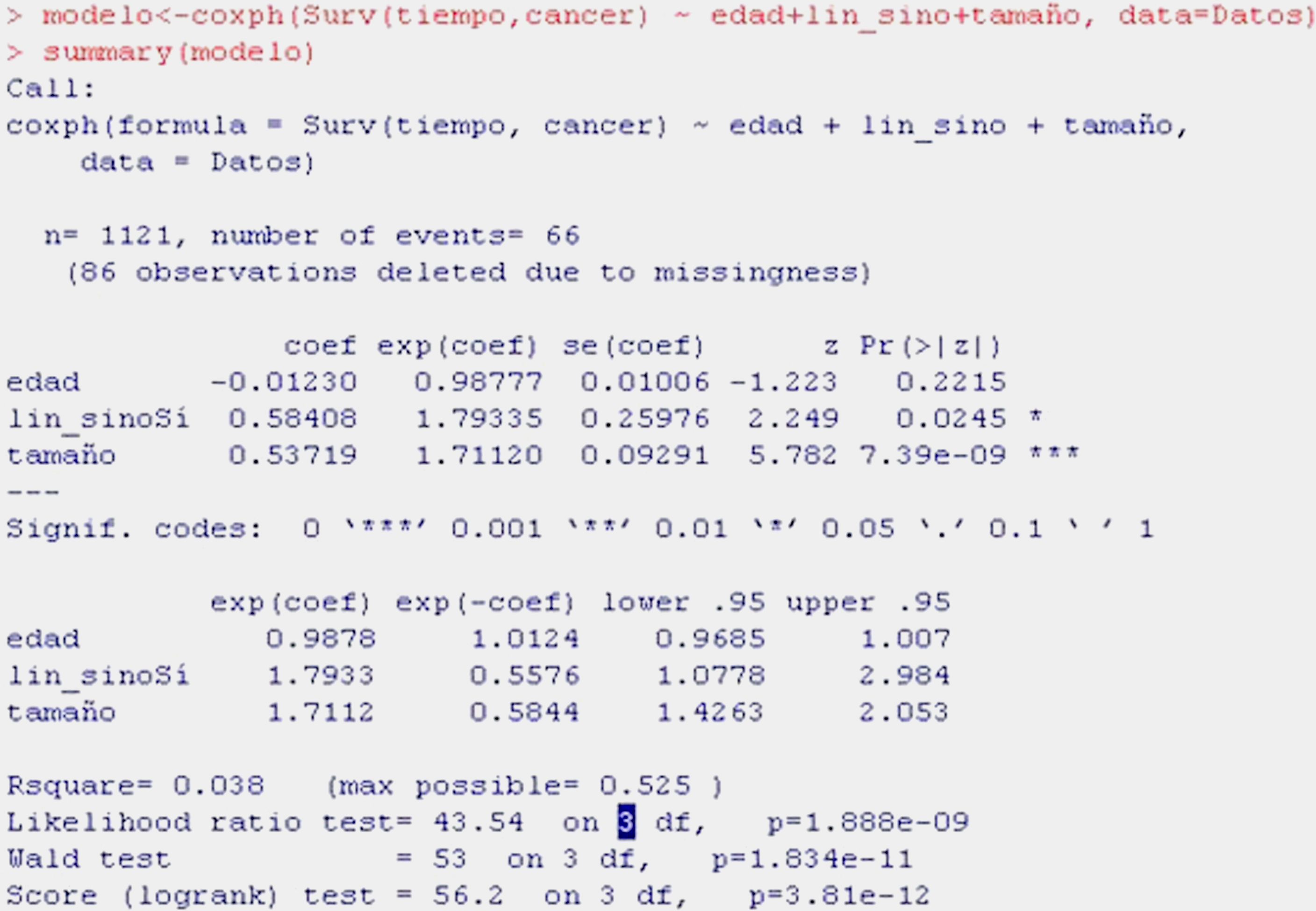
As can be seen from the display, the first information provided is the valid number of cases subjected to Cox regression (1121; 86 lost cases having been excluded); the number of events indicates the deaths caused by breast cancer.
In the table, the first column indicates the coefficients of regression of the model or beta-coefficients, while the following are the relative risk values (HR), standard error, z-value of the test of hypotheses, and the significance of each variable. It is seen that age is not significant (p>0.05), while tumour size and the presence of adenopathies are significant. The HR of the variable presence of adenopathies is 1.7933 – indicating that there is 79% greater risk of death due to breast cancer in the presence of adenopathies versus patients without adenopathies, on fitting for the other two variables, i.e., for equal age and tumour category. The HR of 1.7112 for tumour size means that for each centimetre increase in tumour size, there is a 71% increase in risk of dying due to breast cancer, fitting for age and adenopathies.
The next table shows the same values of relative risk and 1/RR, as well as the confidence interval. The ratio 1/HR is useful for interpreting the variables that constitute protective factors, such as for example age (HR in the previous table <1); 1/0.9878 is equal to 1.0124 and indicates that for each year elapsed, the risk of dying decreases almost 1%, though this variable is not significant (the interval contains 1).
The last information shown is the coefficient of determination R2 and three tests of hypotheses that are significant, and thus corroborate the logic of considering a Cox regression model.
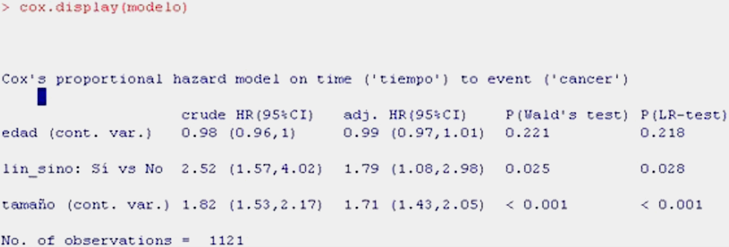
For obtaining a summary of the model with a more clinical perspective, we use the function cox.display of the epicalc package,15 as shown in Table 11.

The information shown is the same as in the previous table, although in summarised form.
The first column shows the raw HR value, which would be the HR without fitting, i.e., that considered for a univariate model where regression is carried out with each of the independent variables individually. The second column corresponds to the adjusted HR, i.e., the value of HR of each variable fitted for the remaining variables of the model. The third and fourth columns in turn indicate the significance of each of the variables according to the Wald statistic and likelihood ratio, which reflect the significance of each variable in the model. Lastly, we can plot the survival curve associated to the fitted model (Fig. 8).
Software
For development of the examples, use has been made of the shareware application R, together with the survival, foreign and epicalc libraries.
Conflict of interestThe authors have no conflict of interest to declare.
Sabina Perez-Vicente holds a contract as research support technician, financed by the Instituto de Salud Carlos III and the Consejeria de Salud de la Junta of Andalucia (Spain).
