


Systematic error, or bias, is error that occurs in each measurement made and which has a direction, i.e., the measured value is always either greater or smaller than the true value. The presence of systematic error directly affects the internal validity of the study, and indirectly affects the external validity of the results obtained. In general, such error can be classified as selection bias, classification bias or confounding bias.
It is essential to deal with possible bias in the research design phase, since only confounding bias can be controlled in the phase corresponding to analysis of the results.
In much of epidemiological research, the aim of the study is to determine the effect of a type of exposure upon a given health problem. The comparison of groups is the fundamental element used to establish causal relationships. Due to the inclusion of errors, all studies are characterised by differences between the observed results and the true results.1 Such errors in turn are of two kinds: (I) random errors; and (II) systematic errors.
Random error affects the precision of the measurements, and is directly related to the study sample and its size. Thus, random error decreases on increasing the size of the study sample or population; it is not constant in each measurement, and does not always occur in the same direction. The use of statistical tools allows us to control random error (precision) – fundamentally by calculating the sample size in the study design phase, including hypothesis tests, and calculating the confidence intervals in the analysis of the results.1
In contrast to the above, systematic error or bias is error that occurs in each measurement, and has a concrete direction, i.e., the measured value is always either greater or smaller than the true value. Thus, the presence of systematic error directly affects the internal validity of the study, and indirectly affects the external validity of the results obtained. Bias can originate in any phase of the investigation, from the selection of the literature used to the establishing of a conceptual frame or setting for the study, to the selection of patients, the measurement processes, and even the publication phase.
A range of biases have been described in the scientific literature, although in general they can be classified as selection bias, classification bias or confounding bias.
Selection biasSelection bias refers to any error derived from identification of the study population. It is an example of systematic error introduced during screening (selection) or follow-up of the population, and which facilitates wrong conclusions referred to the hypothesis being investigated.2
Selection bias appears when the people included in the study differ in terms of some relevant feature or characteristic from the population to which the drawn conclusions are applied.1 It can appear in any epidemiological study, but is more common in cross-sectional studies, when the information is collected by means of a survey.
The common element shared by the different forms of selection bias is that the relationship between exposure and the disease differs in the subjects participating in the study with respect to those subjects which while eligible, are not included in the study. Sackett defined up to 35 different types of selection bias,3 although in this article we will deal with those most commonly found in the medical literature.
Prevalence or incidence bias (Neyman bias)This type of bias occurs when we study a disease that causes early death, and at the start of the study the deceased individuals can no longer be included in the case group.4
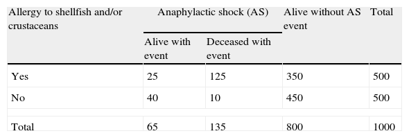
In the following example, a study was made of the relationship between allergy to shellfish and/or crustaceans and the risk of anaphylactic shock (AS), based on the following comparison: a group of 500 individuals with allergy to shellfish and/or crustaceans, and 500 individuals without allergy, followed-up over a period of five years. The data are reflected in Table 1.
Frequency of anaphylactic shock according to the presence or absence of the risk factor (allergy to shellfish and/or crustaceans), in a five-year cohort study.
| Allergy to shellfish and/or crustaceans | Anaphylactic shock (AS) | Alive without AS event | Total | |
| Alive with event | Deceased with event | |||
| Yes | 25 | 125 | 350 | 500 |
| No | 40 | 10 | 450 | 500 |
| Total | 65 | 135 | 800 | 1000 |
From the analysis of the table, the patients with allergy to shellfish and/or crustaceans are seen to be at an increased risk of suffering AS (30%) compared with those without allergy (10%). For an odds ratio (OR) of 3.85 and a 95% confidence interval (CI) of (2.80–5.31),5 the subjects with allergy to shellfish and/or crustaceans have a 3.85-fold higher risk of developing AS than those without allergy.
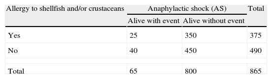
The above example can also be regarded as a case–control study between the subjects that survived after the five years of follow-up (presenting AS or not). The analytical data are shown in Table 2.
Frequency of anaphylactic shock according to the presence or absence of the risk factor (allergy to shellfish and/or crustaceans). Case–control study.
| Allergy to shellfish and/or crustaceans | Anaphylactic shock (AS) | Total | |
| Alive with event | Alive without event | ||
| Yes | 25 | 350 | 375 |
| No | 40 | 450 | 490 |
| Total | 65 | 800 | 865 |
The resulting measure of association (odds ratio) yields a value of 0.80 (95%CI 0.48–1.35). It is therefore wrongly concluded that the presence of the risk factor (allergy) reduces the risk of developing AS. This unexpected result is the consequence of a poorly designed case–control study, due to failure to include in the analysis those individuals that died prematurely because of AS.
Admission rate bias (Berkson bias)This type of bias is defined as the series of selection factors that lead to systematic differences between the hospital cases and controls in a case–control study design.6 Bias occurs when the cases and/or controls are recruited from among hospitalised patients.7
Admission rate bias was described by Berkson in 1946 on evaluating a case–control study in which the conclusion was drawn that tuberculosis exerts a protective effect against cancer. The frequency of tuberculosis in hospitalised cancer patients was found to be lower than the frequency of tuberculosis among hospitalised controls without cancer. These unexpected results were due to the fact that a comparatively smaller proportion of patients with both diseases were hospitalised, and thus served as subjects amenable to inclusion as cases in the study.8
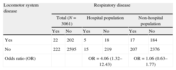
Roberts et al. published the first empirical study demonstrating Berkson bias, affecting the relationship between respiratory diseases and diseases of the locomotor system. In the study published by Roberts, involving a sample of 2784 subjects, 257 individuals had been admitted to hospital in the six months prior to the study.9 The data in Table 3 correspond to the global population and the subgroup of hospitalised individuals with respiratory diseases and diseases of the locomotor system in the study of Roberts.
Locomotor system disease as a risk factor for respiratory disease.
| Locomotor system disease | Respiratory disease | |||||
| Total (N=3061) | Hospital population | Non-hospital population | ||||
| Yes | No | Yes | No | Yes | No | |
| Yes | 22 | 202 | 5 | 18 | 17 | 184 |
| No | 222 | 2595 | 15 | 219 | 207 | 2376 |
| Odds ratio (OR) | OR=4.06 (1.32–12.43) | OR=1.06 (0.63–1.77) | ||||
A strong positive association was observed between the presence of respiratory diseases and the presence of locomotor diseases in the hospitalised individuals. However, Roberts found the respiratory diseases and locomotor disorders to be independent.10
This false association between respiratory diseases and diseases of the locomotor system was found in the hospitalised group because the hospital admission rate among people with both diseases (29.41% [(5/17)×100]), was approximately three times greater than the rate in the rest of the hospitalised patients (patients with only respiratory disease, only locomotor disease, or neither of the two diseases) (9.1% [(252/2767)×100]).
Admission rate bias can be avoided by selecting the controls from among people admitted to the hospital in the same period of time but due to other causes, i.e., selecting the controls from different departments in order to ensure a great variety of diseases, and excluding diagnoses positively or negatively related to the risk factor being studied. The diseases included as controls must present a probability of admission to hospital similar to that of the cases.1
An alternative for solving the problem posed by this kind of bias is the use of two control groups.
Non-response biasNon-response in a survey is defined as failure to secure the participation of all the selected sample units, and represents a growing problem in population-based surveys.11,12
A distinction must be made between non-response to certain items of the questionnaire (missing values) and non-response to most or all the items contained in the questionnaire.
The population estimations obtained from the sample of subjects that answer the questionnaire may differ from the estimations that would have been obtained if the total sample had answered the questionnaire. This difference is known as non-response bias, and occurs when the subjects that fail to respond differ systematically from those who do respond, in reference to those characteristics that are of interest in the study.13,14
In clinical trials (CTs), the studied patients must constitute a representative sample of the individuals that present the problem being studied, or at least of those to whom the evaluated indication is aimed.1 Those subjects who refuse to participate in the study represent a serious problem in CTs.
In a questionnaire assessing allergy prevention habits, aimed at patients with allergy to different types of pollen (cases) and to individuals without allergy (controls), conducted in a city in the south of Spain, the response rate among men was found to be far lower than the response rate among women. This low male participation is explained by the fact that most allergic men do not adopt preventive measures (use of a mask, avoidance of open-air exercise, wearing of sunglasses, etc.) in the months of maximum pollination, while those who are not allergic feel that no preventive measures are needed because they consider themselves to be healthy.
Although it is not possible to avoid non-response bias, its impact can be attenuated by using corrective strategies. A common practice is sample substitution, in which the non-responders are replaced by individuals randomly selected from the study sample setting, or by individuals with characteristics similar to those of the non-responders (matched replacements).15 In CTs, this strategy is used in intention to treat analysis (ITT), where the subjects of the experimental groups that have been lost are included in the analysis as failures, while those lost in the conventional group are included as successes. This analysis is regarded as one of the cornerstones in the analytical strategy of CTs, since it allows us to preserve the benefits of random assignment.16
Information or wrong classification biasInformation bias is defined as bias introduced by the method used to collect information referred to exposure, the results or other confounding or effect-modifying variables. There are two types of information bias: non-differential and differential. Differential information bias is the term used when the magnitude of the bias is related to exposure to the study factor on the part of the subject or the condition of his or her disease, i.e., that where the error is more frequent in some of the study groups.1
In contrast, non-differential information bias is bias that affects all the comparator groups equally, tending to dilute the true existing association (e.g., by hiding or exaggerating sexual risk behaviours).
There are two sources of information bias in epidemiological studies, referred to the participant and to the interviewer, respectively. Examples of each of these forms of bias are given below.
Memory bias, participant biasAs an example, we use a case–control study17 analysing the causal relationship between the eating habits of the mother during pregnancy and the subsequent presence of allergies in the child. The information referred to exposure is that supplied by the mother. In this context, it is understandable that women with allergic children will remember better, or make a greater effort to remember, their eating habits during pregnancy than women with healthy children (differential bias). This example defines a common type of bias in research: memory bias.
The only way to control such bias, in a study of this kind, would have been to adopt a cohort study design with a control group, and subject the mothers to follow-up during the nine months of pregnancy, with subsequent follow-up of the child until the possible allergies develop.
In the aforementioned case, conducting the study as a prospective cohort survey would have been ideal for controlling information bias, but this is not always possible, due to reasons of cost and time. However, what we can do is correctly measure or collect the information supplied by both groups, i.e., adopting an objective and validated tool to ensure that the mothers with allergic children and mothers of healthy children remember their eating habits during pregnancy.
These tools, whether questionnaires, interviews or measurement scales, etc., must be administered by persons trained in their use.
Interviewer or observer biasAnother type of information bias refers to observer or interviewer bias. An example of this is provided by an investigation in which one group of allergic children receives a new drug treatment and another receives the usual drug treatment. If the investigator is also the observer, he or she will tend to be more meticulous in evaluating the new drug treatment group than the other group, even if not deliberately so.
The appropriate approach in the above example would be to consider a clinical trial in which all the assumptions of the latter are implemented: sample randomisation and the adoption of blinding or masking measures, i.e., the way to prevent this type of bias would be to mask both patient and observer assignation (in some cases even the evaluator is blinded).
Another aspect to be taken into account in order to eliminate or prevent information bias is initial evaluation of the concordance or agreement among the measurements of the evaluators. To this effect, before starting the field work, the latter must be trained in correct usage of the instrumentation and determinations.
In sum, information bias can only be evaluated and controlled in the study design stage.
Confounding biasConfounding bias is a distortion of the study estimations produced by the uneven or unbalanced distribution in the comparator groups of a third variable, known as the confounding variable. If this confounding variable is a predictor of effect, then its uneven distribution will contaminate the true relationship between exposure and the evaluated effect or result. Thus, the presence of an uncontrolled confounding variable may lead to the assumption of an effect which in fact does not exist, or may exaggerate or dilute the true relationship existing between the factor and the effect.
In practically all studies, subject age and gender are confounding variables.18 In addition to these variables, smoking habit is a classical confounding variable of obliged consideration when designing epidemiological studies. Other potentially confounding variables that must be taken into account in study data collection are socioeconomic level, ethnic group (race) or place of residence.
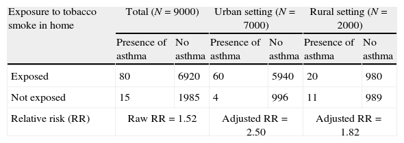
An example of confounding variable is a cohort study in which patients under 14 years of age were followed-up on for one year. The purpose of the study was to determine the association between exposure to tobacco smoke in the home and the development of asthma in childhood in Nicaraguan populations (Fig. 1).

The relative risk (RR) for the development of asthma among the subjects participating in the cohort was 1.52 in favour of those with exposure to smoke in the home.5 However, since the participants belonged to both the rural and urban settings, this fact or variable should have been taken into account in the analysis, due to the greater environmental pollution in urban areas, and to possible differences in smoking habit (see Table 4).
Raw and adjusted relative risk values in an example of confounding factor.
| Exposure to tobacco smoke in home | Total (N=9000) | Urban setting (N=7000) | Rural setting (N=2000) | |||
| Presence of asthma | No asthma | Presence of asthma | No asthma | Presence of asthma | No asthma | |
| Exposed | 80 | 6920 | 60 | 5940 | 20 | 980 |
| Not exposed | 15 | 1985 | 4 | 996 | 11 | 989 |
| Relative risk (RR) | Raw RR=1.52 | Adjusted RR=2.50 | Adjusted RR=1.82 | |||
After stratification according to place or residence, the adjusted RR values are greater than the raw values; as a result, failure to take into account the confounding variable (place of residence) in the analysis dilutes the association between exposure to tobacco smoke in the home and the development of asthma.
Rothman established three conditions for identifying a potential confounding variable: (I) it must be a predictor of effect even among the subjects not exposed to the study factor; (II) it must be associated to the exposure under study, including the subjects that do not develop the effect; and (III) a confounding variable cannot be the intermediate step in the causal sequence between exposure and the effect or disease under study (e.g., the blood cotinine value in children between a cause such as exposure to tobacco smoke in the home and the development of asthma in childhood).19
Confounding bias is the only one of the three types of bias that can be controlled both in the study design phase and posteriorly in the analytical phase of an epidemiological study.20 In the design phase, the methodological variants aim to prevent the occurrence of such bias, with the adoption of three possible types of strategies:
- (I)
Randomisation. This is one of the fundamental elements in experimental designs. Randomisation involves the random assignation of the study subjects to the different comparator groups. Thus, any confounding factor (known or otherwise) can be taken to be homogeneously distributed among the different groups as a result of the randomisation process – thereby minimising the possibility that the confounding variable is associated to the exposure under study.
- (II)
Restriction. This involves restricting the subject admission criteria according to the potential confounding variable.19 In general, we select a single specific category for nominal variables (e.g., sex or race), or a narrow range for potential quantitative confounding variables (e.g., age or years of exposure to tobacco smoke). Restriction can be implemented in analytical and experimental designs, and contributes to ensuring that the confounding factor does not exhibit a heterogeneous distribution among the different comparator groups.
- (III)
Matching. This is an alternative to restriction, used in both analytical and experimental studies, in which each subject of the exposure group is matched to one or more subjects in the non-exposed group, in one same confounding factor category. Matching can be made for one or more potential confounding factors, and the subjects compared can be matched either individually or by groups. Common matching variables are sex or age groups.
Likewise, in the analytical phase, confounding bias can be controlled by resorting to:
- (I)
Stratification. Stratified analyses provide estimations of the measures of association in the different levels of the confounding factor which we wish to control. The advantage of stratification is that it allows better knowledge of the data and the detection of possible interactions. In contrast, when we wish to analyse multiple variables and categories, strata of insufficient size may be generated.21
- (II)
Multivariate analysis. The most efficient alternative for determining the existence of possible confounding variables is multivariate analysis, since it allows the simultaneous evaluation of different variables. Depending on the response or dependent variable of the study, use is made of logistic regression,22 survival,23 or linear regression models,24 among others.
For one same sample size, the set of variables associated to the outcome (model) extracted from an initially important number of variables through the multivariate analysis affords more precise estimations, and with more variables than stratified analysis.
- (III)
Standardisation. In ecological designs, use is made of the adjustment or standardisation of mortality rates,25 with the purpose of homogenising the confounding variable in the different comparator groups (e.g., age).
In general, a confounding factor is considered to be present when important differences are observed between the raw estimations of a given association and the estimations obtained after adjusting for possible confounding variables. Thus, a variable is statistically identified as being a confounding element when the magnitude of the difference between the two estimations is at least 10%, as used in the statistical analyses, and presents a conservative level of significance of under 0.20.26
Final commentsThe knowledge, prevention and control of the effects of bias will allow a correct approach to research studies, with correct interpretation of the results of the scientific publications.
It is essential to deal with possible bias in the research design phase, since only confounding bias can be controlled in the phase corresponding to analysis of the results.
Conflict of interestThe authors have no conflicts of interest to declare.
Sabina Perez-Vicente holds a contract as research support technician, financed by the Instituto de Salud Carlos III and the Consejeria de Salud de la Junta de Andalucía (Spain).
Thanks are due to Nicolás Benítez-Parejo for reading the different manuscript drafts.
