


The aim of this article is to analyze the determinants of celibacy at 45 years of age in the generations born between 1785 and 1965. Men and women will be analyzed separately, based on individual variables, such as family, economic, nutritional, physical and behavioural factors. To do this we will divide the period into two sub-periods, one pre-transitional (born between 1785 and 1900) and another transitional and post-transitional (born between 1900 and 1965). The microdata for the analysis comes from nine rural municipalities of the region of Aragon, in north-eastern Spain. The results will highlight the influence of the family, economic, nutritional and physical contexts on the marital status at the age of 45.
El objetivo de este capítulo es analizar los determinantes del celibato a los 45 años en las generaciones nacidas entre 1785 y 1965. Analizando por separado a hombres y mujeres, en base a variables individuales, familiares, económicas, nutricionales, físicas y de comportamiento. Para ello, vamos a dividir el período en dos subperíodos, uno pretransicional (nacidos entre 1785 y 1900) y otro transicional y postransicional (nacidos entre 1900 y 1965). Los microdatos para el análisis provienen de nueve municipios rurales de la región de Aragón, en el noreste de España. Los resultados destacan la influencia del contexto familiar, económico, nutricional y físico en el estado civil a los 45 años.
During the Middle Ages emerged, in western Europe, what John Hajnal (1965) has called the Western European Marriage Pattern. This model was characterized by an increase in the age at when people first married, as well as an increase in the rate of celibacy, especially female celibacy, which increased from 1% to more than 10% (for a comparison of European and Asian locations in the pre-transitional period, see Dribe et al., 2014). Authors such as Malthus (1798–1992) have indicated these mechanisms (increase in the age of marriage and in the rate of celibacy) as among the reasons for the decrease of fertility and mortality throughout Europe. The increase in the age of marriage, as well as the high proportion of those remaining unmarried, would have effectively reduced the fertility rate. Thus, the overpopulation that led to violent outbreaks of disease associated with overcrowding became avoidable. The increase in numbers of those who remained single did not arise from any social pact for controlling population excesses, but rather – comparable to the age of marriage – was determined by a set of social norms that governed the marriage market (Dribe and Lundh, 2014). These social norms were related to factors such as social and family position, health, the environment and social respectability. Although we cannot measure all these determinants, we will approach them through different indicators (individual, familial, economic, epidemiological, nutritional and physical). Thus, the aim of this study is to define the determinants of celibacy at the age of 45 for both men and women born between 1785 and 1965. By this method we will attempt to answer the question of whether rural societies shared the same determinants of celibacy as other areas of the European continent. As the bibliography shows, Spain did not fully adopt the European Marriage Pattern, although the average age at first marriage and the rate of remaining single during these centuries did increase slightly (see Reher, 1991). This article aims to provide new evidence on remaining single in Spain, and to analyze those factors that gave rise to this increase.
We will use the terms the single state and celibacy without distinction. When using them we will be referring to reaching the age of 45 without having married, since the possibilities for people of this age to start a family and to bear children will have been considerably reduced. We will examine the determinants of the single state in nine rural villages in the province of Zaragoza. Based on available data, we will consider only the determinants of celibacy in native individuals who did not migrate. Devos et al. (2016), in a recent publication, have highlighted the paucity of existing work on the single state and its determinants. This shortage of research is even more palpable for the Spanish case.
Some of the variables used in this study are being applied for the first time in the study of celibacy, while others have been used in different geographical or temporal contexts. Among these variables is male height in the twentieth century. They serve as a high-quality proxy for health and nutritional status. In this context, the Demographic Transition that began in the area in the early twentieth century assumed a revolution at the family and economic levels (Marco-Gracia, in press). Because of this, the analysis has been carried out for two separate periods: pre-transitional (1785–1899), and transitional (1900–1965).
2Materials: area and dataThe study area includes nine rural villages in the northeast of Spain: Alfamén, Botorrita, Jaulín, Longares, Mezalocha, Mozota, Muel, Tosos and Villanueva de Huerva (see Fig. 1). In municipal terms they occupy an area of 500km2 around the middle valley of the Huerva River. The database ‘Alfamén & Middle Huerva Database’ (AMHDB) was constructed based on individual information from the parish records of baptisms, marriages and deaths for the period between 1473 and 1950. The archives for this period are of a very high quality. The central inherent problem of the Spanish Catholic archives comprises the under-registration of the birth of females; in this period (1785–1965) the births of 106.7 boys per 100 girls are registered. For the period from 1951 until 2012 the database was completed by means of individual interviews centred on the same information guidelines. Individual data were pooled following the family reconstruction method developed by Fleury and Henry (1956), and included 95,817 individuals. This area had a total of 5,486 inhabitants in 1780, 5,884 in 1860, 8,086 in 1950 and 5,444 in 2012. Rural–urban migrations have seriously affected some municipalities during the course of the twentieth century.

The study area is located on the Ebro Valley at the foot of the Algairén Mountains. The distance to Zaragoza varies from 19.75 to 40km. Its inhabitants are traditionally agricultural, managing chiefly cereal fields and vineyards. The area also has sheep grazing pasture. Data on occupations and literacy have been extracted from population censuses (1857, 1860), electoral rolls (1890, 1894, 1900, 1910, 1920, 1930, 1934, 1945, 1951 and 1955), the population register of 1824, and more rarely, from church registers and interviews. Information on professions and literacy was linked to the life patterns for each individual. Professions have been categorized into five groups. The first group, ‘day-labourers’, includes landless agricultural labourers, small landowners and other workers, such as unskilled labourers. Ordinarily, day-labourers combined agricultural tasks with small jobs in times of lesser agricultural activity. The second category, ‘farmers,’ includes all landowners who could support themselves exclusively from their farms. The third group, ‘shepherds’, includes all herder of sheep and goats, regardless of whether or not they are owners of livestock. The fourth group, ‘artisans’, consists of non-agricultural workers engaged in manual production (potters, bakers, blacksmiths, glaziers, etc.). The fifth category, ‘highly qualified’, includes non-manual professions of high social prestige in rural areas (doctors, veterinarians, teachers, bankers, etc.), all of which require a high level of education. The rest of the professions (military, public servants, drivers, etc.) have been included in the ‘other’ category, along with individuals who we do not aware of their occupation.
In a large part of Aragon, including this area, the inheritance was divided equally between sons and daughters. This transmission of family wealth was made at the time the descendant contracted their marriage, through the dowry, or at the end of their life, through the will.
For the analysis of the determinants of celibacy, we have added to the database two complementary variables from the military conscription details of each man: height adjusted according to age, and reasons for not entering military service.1 The analysis only includes those native individuals whose birth dates are known. We calculate the time in days from the measurement to attaining 21 years of age. Sanz-Gimeno and Ramiro-Fariñas, 2002 indicate that growth rates can continue up until 21 years, when the maximum height is reached. In order to adjust the height of all individuals to this maximum, the recorded height was compensated for by adding 0.0273785mm for each day until the age of 21 (an adjustment of 1cm per year). This is clearly an imperfect adjustment, since different people grow at different rates depending on their genetic and biological conditions. No compensation was made if the individual was measured after the 21 years. Extreme cases of less than 1.300m and greater than 2m were withdrawn. After adjusting the height of each individual, the adjusted height was compared with the average height of those born during the same quinquennial (beginning in 1900–1904 and ending in the extended period 1960–1965). From this comparison, the distance in millimetres from the five-year average was obtained by using the methodology proposed by Reher and Ortega (2004). These distances were arranged into five groups, with a relatively homogeneous number of cases: 1 – very low, more than 45mm below average; 2 – low, between 45mm and 15 below average; 3 – common, between 15mm below average and 8 above; 4 – high, between 8mm and 35 above the average; and 5 – very high, more than 35mm above the average. Regarding the reasons for not entering military service, these were grouped into 7 categories: 1 – temporary physical illness or problems, but of sufficient gravity to be grounds for exemption; 2 – moderate physical problems (such as sight or hearing problems); 3 – severe physical problems (such as blindness or serious physical incapacity); 4 – physical problems poorly defined; 5 – family poverty (mainly due to incapacity of the father or the widow of the mother); 6 – having brothers serving in the army; 7 – no motive put forward. These categories follow the proposal of Ayuda and Puche (2014) for the Valencian records.
In order to study the influence of the economic context during the years of birth and the following years, a variable has been included on the fluctuation of wheat prices in the city of Zaragoza for the pre-transitional period (the series has been extracted from: Peiró, 1987). We have taken the development of prices, once the trend of the wheat prices was removed through a logarithmic basis. We have considered the possibility of a subsistence crisis when prices were at least 10% higher than the average for the period.2 This criterion has been used in many international articles, as it is a threshold that affects the standard of living (for more information on its justification and use, see Bengtsson et al., 2004). We wish to examine whether having been born in the year of a subsistence crisis (or one or two years before it) affected the chances of individuals marrying before the age of 45.
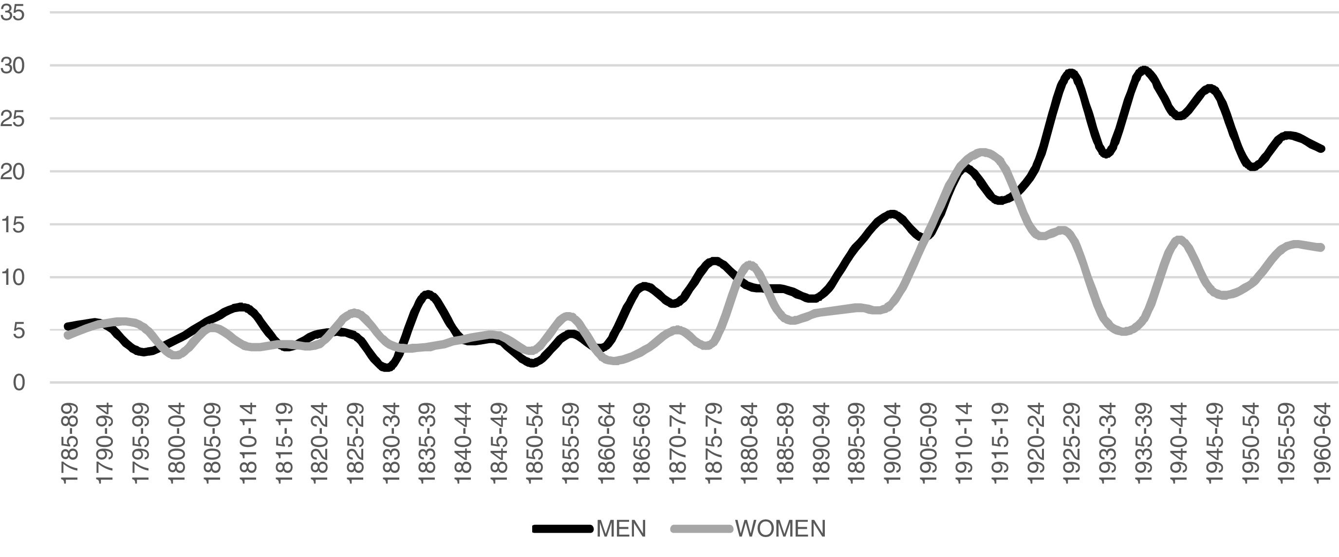
We can observe in Fig. 2 that the rates of remaining single for men and women over 45 years have been similar from the end of the eighteenth century to the quinquennium 1860–1864. From that moment onwards, the male rates began to differ from the female rates, although it was not until the quinquennium 1915–1920 when the graph curves for men and women separated indefinitely. This trend is explained to a large extent by the rates of female migration, which have been higher than the male rates since the second half of the nineteenth century. Cities had become centres of population attraction, and some of these families required maids, mainly from the surrounding villages. Thus, while in Spain as a whole the rate for females remaining single was higher than that for men (Reher, 1991: 15), in those municipalities analyzed we find the opposite effect. During the 1970s the greatest rate of female outmigration was heralded by the arrival of new ideas linked to the Second Demographic Transition, which not only changed attitudes towards marriage and the single state, but also encouraged females to take up new urban jobs. The figures for those remaining single in the study area during the nineteenth century were low, close to the Spanish average of around 7.3% for men and 10.9% for women in 1887 (Reher, 1991), and below that of other European locations between 1716 and 1913, such as Casalguidi in Italy with 17.1% men and 10.3% women, Sart in Belgium with 18.2% men and 14% women, or some localities in the south of Sweden, with 12.8% men and 20.5% women (Dribe et al., 2014).
3Methodology.")
The raw material for this study comprises unmarried people over 45-years-old, born between 1785 and 1965, and who did not dedicate their adult life to a religious vocation. The selection criteria, only individuals over 45-years-old, could have underestimated the coefficients of some of the variables by reducing the number of individuals in the sample. Among those individuals, and in order to identify celibates we take all those individuals whose date of birth is known to us, namely the natives. We must also consider that they either continued to reside in one of the sample villages or, if deceased, that their dates of death are known. We therefore omit all those who migrated. We know that day-labourers and the daughters of day-labourers migrated in higher numbers, since they were less tied to the land through land ownership (Marco-Gracia, 2017). Our interest is in knowing the marital status of natives at the age of 45, so that those who died before reaching that age are excluded from the sample. In order to know the effect of parental longevity on single people, given the relevant role played in the Netherlands (Kok and Mandemakers, 2016), if we simply do not know the exact age of death, then we accept the age recorded by the parish priest as an approximation. In order to complete the remaining variables on the family context (numbers of unmarried siblings, numbers of deceased siblings, parity, etc.) we need parents who have remained in the locality, and so we only take into account those individuals of whom we have information on their parents.
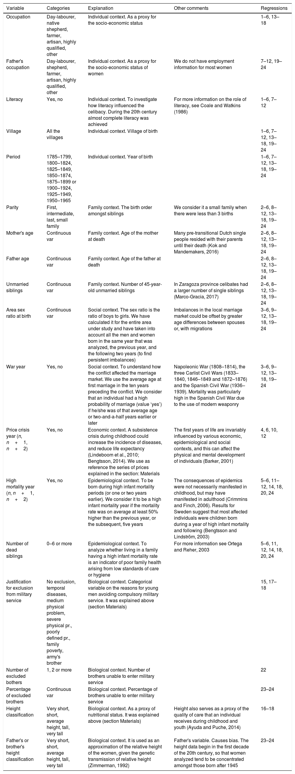
In this article we only analyze contextual, socio-economic and physical variables because other relevant variables are unavailable, such as those related to the character of individuals. It is also of great interest to understand how the context influences the potential of each individual to remain celibate. Our approach to these determinants will employ logistic regressions. We will take as a dependent variable the fact of being or not being single at 45 years of age. It requires a ‘zero’ value to have married, and a ‘one’ to remain celibate. In other words, the dependent variable analyses marital success. To better understand the effect of the different variables, we will group the regressions (in groups of six) into hierarchical models by gender and period. In each regression, we will introduce new variables to interact with those previously studied. Four groups of regressions have been developed: men 1785–1899 (regressions 1–6), women 1785–1899 (regressions 7–12), men 1900–1965 (regressions 13–18), and women 1900–1965 (regressions 19–24). The regressions include the following variables: Table 1.
Description of the variables included in the models.
| Variable | Categories | Explanation | Other comments | Regressions |
|---|---|---|---|---|
| Occupation | Day-labourer, native shepherd, farmer, artisan, highly qualified, other | Individual context. As a proxy for the socio-economic status | 1–6, 13–18 | |
| Father's occupation | Day-labourer, shepherd, farmer, artisan, highly qualified, other | Individual context. As a proxy for the socio-economic status of women | We do not have employment information for most women | 7–12, 19–24 |
| Literacy | Yes, no | Individual context. To investigate how literacy influenced the celibacy. During the 20th century almost complete literacy was achieved | For more information on the role of literacy, see Coale and Watkins (1986) | 1–6, 7–12 |
| Village | All the villages | Individual context. Village of birth | 1–6, 7–12, 13–18, 19–24 | |
| Period | 1785–1799, 1800–1824, 1825–1849, 1850–1874, 1875–1899 or 1900–1924, 1925–1949, 1950–1965 | Individual context. Year of birth | 1–6, 7–12, 13–18, 19–24 | |
| Parity | First, intermediate, last, small family | Family context. The birth order amongst siblings | We consider it a small family when there were less than 3 births | 2–6, 8–12, 13–18, 19–24 |
| Mother's age | Continuous var | Family context. Age of the mother at death | Many pre-transitional Dutch single people resided with their parents until their death (Kok and Mandemakers, 2016) | 2–6, 8–12, 13–18, 19–24 |
| Father age | Continuous var | Family context. Age of the father at death | 2–6, 8–12, 13–18, 19–24 | |
| Unmarried siblings | Continuous var | Family context. Number of 45-year-old unmarried siblings | In Zaragoza province celibates had a larger number of single siblings (Marco-Gracia, 2017) | 2–6, 8–12, 13–18, 19–24 |
| Area sex ratio at birth | Continuous var | Social context. The sex ratio is the ratio of boys to girls. We have calculated it for the entire area under study and have taken into account all the men and women born in the same year that was analyzed, the previous year, and the following two years (to find persistent imbalances) | Imbalances in the local marriage market could be offset by greater age differences between spouses or, with migrations | 3–6, 9–12, 13–18, 19–24 |
| War year | Yes, no | Social context. To understand how the conflict affected the marriage market. We use the average age at first marriage in the ten years preceding the conflict. We consider that an individual had a high probability of marriage (value ‘yes’) if he/she was of that average age or two-and-a-half years earlier or later | Napoleonic War (1808–1814), the three Carlist Civil Wars (1833–1840, 1846–1849 and 1872–1876) and the Spanish Civil War (1936–1939). Mortality was particularly high in the Spanish Civil War due to the use of modern weaponry | 3–6, 9–12, 13–18, 19–24 |
| Price crisis year (n, n+1, n+2) | Yes, no | Economic context. A subsistence crisis during childhood could increase the incidence of diseases, and reduce life expectancy (Lindeboom et al., 2010; Bengtsson, 2014). We use as reference the series of prices explained in the section: Materials | The first years of life are invariably influenced by various economic, epidemiological and social contexts, and this can affect the physical and mental development of individuals (Barker, 2001) | 4, 6, 10, 12 |
| High mortality year (n, n+1, n+2) | Yes, no | Epidemiological context. To be born during high infant mortality periods (or one or two years earlier). We consider it to be a high infant mortality year if the mortality rate was on average at least 50% higher than the previous year, or the subsequent, five years | The consequences of epidemics were not necessarily manifested in childhood, but may have manifested in adulthood (Crimmins and Finch, 2006). Results for Sweden suggest that most affected individuals were children born during a year of high infant mortality and following (Bengtsson and Lindström, 2003) | 5–6, 11–12, 14, 18, 20, 24 |
| Number of dead siblings | 0–6 or more | Epidemiological context. To analyze whether living in a family having a high infant mortality rate is an indicator of poor family health arising from low standards of care or hygiene | For more information see Ortega and Reher, 2003 | 5–6, 11, 12, 14, 18, 20, 24 |
| Justification for exclusion from military service | No exclusion, temporal diseases, medium physical problem, severe physical pr., poorly defined pr., family poverty, army's brother | Biological context. Categorical variable on the reasons for young men avoiding compulsory military service. It was explained above (section Materials) | 15, 17–18 | |
| Number of excluded bothers | 1, 2 or more | Biological context. Number of brothers unable to enter military service | 22 | |
| Percentage of excluded brothers | Continuous var | Biological context. Percentage of brothers unable to enter military service | 23–24 | |
| Height classification | Very short, short, average height, tall, very tall | Biological context. As a proxy of nutritional status. It was explained above (section Materials) | Height also serves as a proxy of the quality of care that an individual receives during childhood and youth (Ayuda and Puche, 2014) | 16–18 |
| Father's or brother's height classification | Very short, short, average height, tall, very tall | Biological context. It is used as an approximation of the relative height of the women, given the genetic transmission of relative height (Zimmerman, 1992) | Father's variable. Causes bias. The height data begin in the first decade of the 20th century, so that women analyzed tend to be concentrated amongst those born after 1945 | 23–24 |
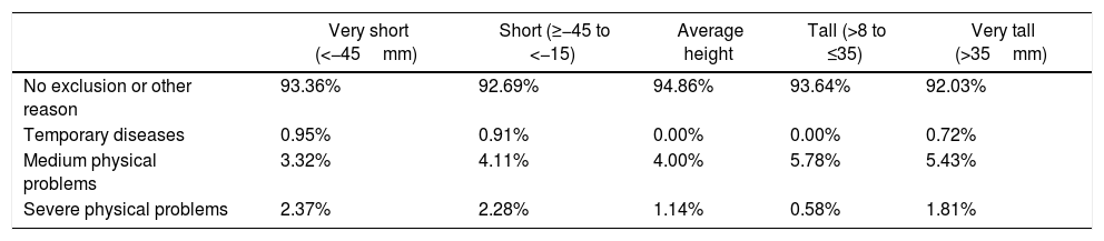
We are going to examine heights and the reasons for avoiding military service separately because some authors have suggested that shorter individuals were more likely to be prone to diseases and other physical problems (e.g. Hacker, 2008; Sohn, 2015). However, as can be seen from Table 2, this relationship is not evident in this study area. Shorter individuals who reached 45 years old did not report any additional physical problems or serious illnesses than other groups. In fact, they were found to be average.
Relationship between height (measured as the distance in millimetres of the individual's height and analyzed according to the average height in the period of his birth) and physical problems given as reasons not to enter military service.
| Very short (<−45mm) | Short (≥−45 to <−15) | Average height | Tall (>8 to ≤35) | Very tall (>35mm) | |
|---|---|---|---|---|---|
| No exclusion or other reason | 93.36% | 92.69% | 94.86% | 93.64% | 92.03% |
| Temporary diseases | 0.95% | 0.91% | 0.00% | 0.00% | 0.72% |
| Medium physical problems | 3.32% | 4.11% | 4.00% | 5.78% | 5.43% |
| Severe physical problems | 2.37% | 2.28% | 1.14% | 0.58% | 1.81% |
We will now analyze the most significant results of the hierarchical models. To do this we will divide the results by the year of birth, 1785–1899 or 1900–1965, depending on gender. We will focus on the variables that appear significant in different logistic regressions, locating similarities and differences between genders and periods. In the analysis of the results, and in each of the following subsections, a summary of the regression results with the most important and significant variables has been introduced (Tables 3–6). The complete regressions are located in the appendices. The bulk of the analysis refers to a society in which the only acceptable marriage was Catholic, heterosexual and monogamous, and to succeed in the local marriage market it was necessary to have an even ratio of the number of possible spouses (Abramitzky et al., 2011).
Odds-ratio of the variables that appear significant in logistic regressions to identify the determinants of male bachelorhood (born between 1785 and 1899). Complete regressions in Appendix A.
| Singlehood | (1) | (2) | (3) | (4) | (5) | (6) |
|---|---|---|---|---|---|---|
| Number of obs. | 2843 | 2843 | 2843 | 2843 | 2843 | 2843 |
| Village | Botorrita (ref.) | |||||
| Longares | 2.03** | 1.93* | 1.91* | 1.93* | 1.89* | 1.90* |
| Mozota | 1.85* | 1.68* | 1.67* | 1.59 | 1.67* | 1.58 |
| Period | 1785–1799 (ref.) | |||||
| 1850–1874 | 1.57 | 1.55 | 1.54 | 1.67* | 1.54 | 1.69* |
| 1875–1899 | 3.90*** | 3.69*** | 3.72*** | 3.90*** | 3.79*** | 3.96*** |
| Parity | First (ref.) | |||||
| Intermediate | 2.28** | 2.22** | 2.28** | 2.30** | 2.35** | |
| Last | 0.25 | 0.10 | 0.14 | 0.08 | 0.12 | |
| Mother age | 1.75* | 1.79* | 1.78* | 1.83* | 1.81* | |
| Father age | 1.78* | 1.83* | 1.85* | 1.86* | 1.89* | |
| Unmarried siblings | 4.79*** | 4.84*** | 4.94*** | 4.67*** | 4.77*** | |
| Area sex ratio | 1.76* | 1.72* | 1.80* | 1.71* | ||
| Price crisis year | No (ref.) | |||||
| Price crisis year | 2.61*** | 2.60*** | ||||
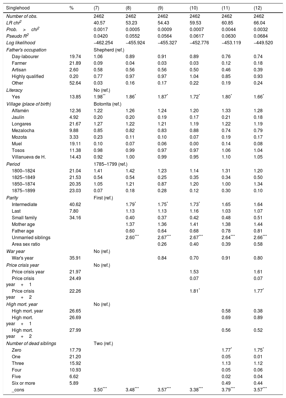
Odds-ratio of the variables that appear significant in logistic regressions to identify the determinants of female spinsterhood (born between 1785 and 1899). Complete regressions in Appendix B.
| Singlehood | (7) | (8) | (9) | (10) | (11) | (12) |
|---|---|---|---|---|---|---|
| Number of obs. | 2462 | 2462 | 2462 | 2462 | 2462 | 2462 |
| Literacy | No (ref.) | |||||
| Yes | 1.98** | 1.86* | 1.87* | 1.72* | 1.80* | 1.66* |
| Parity | First (ref.) | |||||
| Intermediate | 1.79* | 1.75* | 1.73* | 1.65 | 1.64 | |
| Unmarried siblings | 2.60*** | 2.67*** | 2.67*** | 2.64*** | 2.66*** | |
| Price crisis year | No (ref.) | |||||
| Price crisis year | 1.53 | 1.61 | ||||
| Price crisis year+1 | 0.07 | 0.07 | ||||
| Price crisis year+2 | 1.81* | 1.77* | ||||
| Number of dead siblings | Two (ref.) | |||||
| Zero | 1.77* | 1.75* | ||||
| One | 0.05 | 0.01 | ||||
| Three | 1.13 | 1.12 | ||||
| Four | 0.05 | 0.06 | ||||
| Five | 0.02 | 0.04 | ||||
| Six or more | 0.49 | 0.44 | ||||
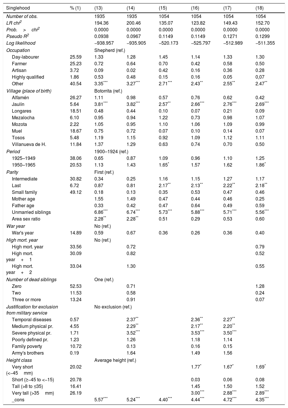
Odds-ratio of the variables that appear significant in logistic regressions to identify the determinants of male bachelorhood (born between 1900 and 1965). Complete regressions in Appendix C.
| Singlehood | (13) | (14) | (15) | (16) | (17) | (18) |
|---|---|---|---|---|---|---|
| Number of obs. | 1935 | 1935 | 1054 | 1054 | 1054 | 1054 |
| Village | Botorrita (ref.) | |||||
| Jaulín | 3.81*** | 3.82*** | 2.57** | 2.66*** | 2.76*** | 2.69*** |
| Period | 1900–1924 (ref.) | |||||
| 1950–1965 | 1.13 | 1.43 | 1.65* | 1.57 | 1.62 | 1.86* |
| Parity | First (ref.) | |||||
| Last | 0.87 | 0.81 | 2.17** | 2.13** | 2.22** | 2.18** |
| Unmarried siblings | 6.86*** | 6.74*** | 5.73*** | 5.88*** | 5.71*** | 5.56*** |
| Area sex ratio | 2.28** | 2.28** | 0.51 | 0.29 | 0.53 | 0.60 |
| Justification for exclusion | No exclusion (ref.) | |||||
| Temporal diseases | 2.37** | 2.36** | 2.27** | |||
| Medium physical pr. | 2.29** | 2.17** | 2.20** | |||
| Severe physical pr. | 3.52*** | 3.53*** | 3.50*** | |||
| Height class | Average height (ref.) | |||||
| Very short (<−45mm) | 1.77* | 1.67* | 1.69* | |||
| Very tall (>35mm) | 3.00*** | 2.88*** | 2.89*** | |||
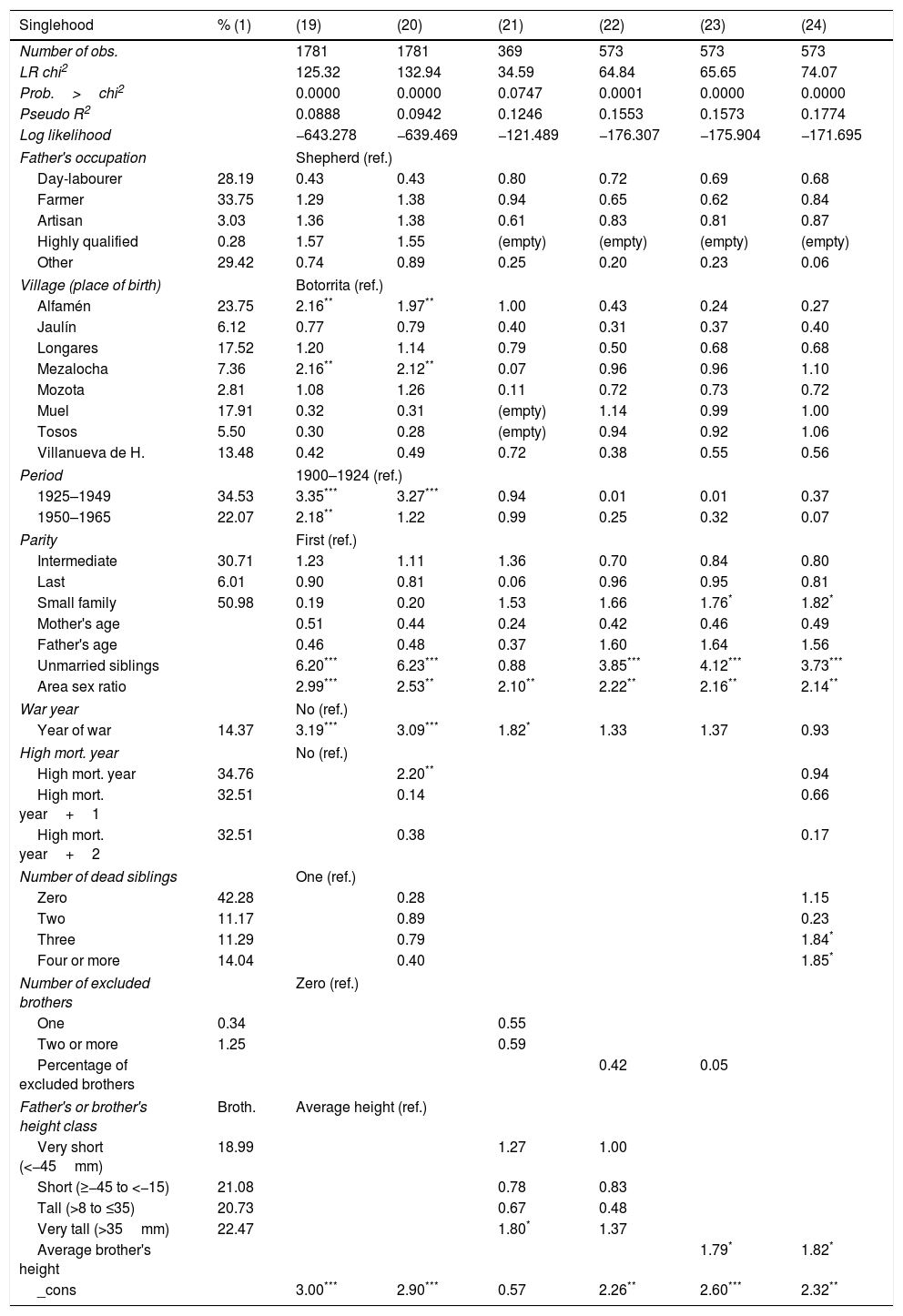
Odds-ratio of the variables that appear significant in logistic regressions to identify the determinants of female spinsterhood (born between 1900 and 1965). Complete regressions in Appendix D.
| Singlehood | (19) | (20) | (21) | (22) | (23) | (24) |
|---|---|---|---|---|---|---|
| Number of obs. | 1781 | 1781 | 369 | 573 | 573 | 573 |
| Period | 1900–1924 (ref.) | |||||
| 1925–1949 | 3.35*** | 3.27*** | 0.94 | 0.01 | 0.01 | 0.37 |
| Parity | First (ref.) | |||||
| Small family | 0.19 | 0.20 | 1.53 | 1.66 | 1.76* | 1.82* |
| Area sex ratio | 2.99*** | 2.53** | 2.10** | 2.22** | 2.16** | 2.14** |
| War year | No (ref.) | |||||
| Yes | 3.19*** | 3.09*** | 1.82* | 1.33 | 1.37 | 0.93 |
| High mort. year | No (ref.) | |||||
| Yes | 2.20** | 0.94 | ||||
| Number of dead siblings | One (ref.) | |||||
| Three | 0.79 | 1.84* | ||||
| Four or more | 0.40 | 1.85* | ||||
| Father's height class | Average height (ref.) | |||||
| Very tall (>35mm) | 1.80* | 1.37 | ||||
| Average brother's height | 1.79* | 1.82* | ||||
The odds ratio of the logistic regressions, contained in Table 3, allow us to better understand the determinants of male celibacy during the pre-transitional period. On the one hand, we note that in the first regression (1) concerning personal characteristics, those individuals having a profession requiring a high level of qualifications were largely celibate. This could be because people of a certain socio-economic status seeking spouses generally belonged to families of equal status (or preferred to marry a person of the same status or the same ideology: Kalmijn, 1994). These individuals are scarce in the study area, so it is difficult to find a spouse with similar characteristics. On the other hand, although it is not highly significant, farmers married in a greater proportion than those with other occupations. This happens in practically all periods for both sexes. Possibly the explanation for this effect is that they were landowners, which meant a degree of insurance against hunger in a low-income context. The place of origin also appears to influence male celibacy. Being born in Longares, a larger location, or Mozota, a smaller village, was linked with remaining celibate.
In the regression (2), and also in the following, we can see that being born into a middle position was related to a lower marriage ratio in the study area. It was those born into small families or in the last position who, in a greater proportion, went on to marry. The sons of long-lived mothers were less inclined to marry, and the same applied to the sons of long-lived fathers. Therefore, the presence of a caring mother or father would have actually lessened the chance of marriage. These results arose from the situation in The Netherlands, where both parents could have influenced long-term celibacy (Kok and Mandemakers, 2016). Another highly significant variable in all models is the number of celibate brothers. Celibate individuals in many cases had celibate siblings. This could be due to two causes. First, some families had serious problems with their children being unsuccessful in the marriage market, whether for economic reasons, or those of social or physical prestige. However, in our study area only two families with four or more children who had reached the age of 45 failed to see any of their children marry. Second, the existence of an unattached brother could have guaranteed a long-term companion in the home, and especially so with the existence of an unmarried sister (Kok and Mandemakers, 2016). At the same time, adult single siblings could have represented an insurance against subsistence crises due to economic reasons during low-income periods.
Among the contextual variables introduced into the model, regression (3)–(6), only two have emerged as significant. The first is the sex ratio of the whole area. The effect is the expected, higher ratio of boys to girls being born, which resulted in imbalances in the marriage market, favoured higher ratio of unmarried men at the age of 45. The second significant contextual variable is that of being born in a year of high wheat prices, a factor that would have some influence on permanent celibacy. The explanation for this could be that children who lived through a subsistence crisis in their infancy received a lower calorie or lower quality diet, and this could certainly influence the future development of such children (Bengtsson et al., 2004). In short, some factors related to childhood could have serious consequences at the time of entering the marriage market.
4.2Determinants of remaining unmarried in women born during the pre-transitional period (1785–1899)Table 4 includes a hierarchical model on the determinants of spinsterhood. The variables included are the same as in Table 3, except for socio-economic status, which in this case was formed with regard to the father's profession as an approach to family socio-economic status. Regression (7) includes the variables on individual context. For women only literacy appears as significant, and is repeated in all the regressions studied in this period. In proportion to the group they represented, there were almost twice as many unmarried women at the age of 45 that were literate rather than non-literate. This has been observed throughout most of the European continent (Coale and Watkins, 1986). Literacy was not excessively important in the marriage market, either for men or women. Among the individual variables – although it is not significant – it is also worth highlighting the case of the daughters of landowner farmers. These women were more successful in the marriage market, with a very low percentage of single women. Perhaps the division of property at the time of the dowry made them more desirable within a context of low-income levels.
In the regression (8) we introduced the family context. In this case, as with men, we note that being neither the eldest nor the youngest sibling would be an influence for marriage. Intermediate children had a lower marriage ratio. This is significant for regressions (8)–(10). Similarly, and also as with men, the presence of single siblings would also have influenced those remaining single. However, the influence of single brothers was lower in the case of women. Although in both cases it was important, the odds ratio reflects double values for men above those for women.
By introducing the epidemiological context in regressions (11) and (12), we note that no deaths of any brother or sister within the family would have favoured permanent celibacy. This could be because families who did not suffer these losses could have attained larger family sizes and therefore, as an unvaried economic reality would have had consequences, suffered from lower living standards.3 At the same time, such low living standards could reduce the potential for accumulating a dowry for a daughter's marriage. Finally, introducing new variables on the economic context at birth, in regressions (10) and (12) we can see that girls who had reached 1 or 2 years of age at a time of economic hardship went on to marry in greater numbers. This is quite contrary to what occurred with men during their first months of life. This effect is difficult to explain. However, we can draw the tentative conclusion that girls were not negatively affected in the marriage market by economic hardship.
4.3Determinants of remaining unmarried in men born in the first two-thirds of the twentieth century (1900–1965)Table 5 contains the odds ratio of six logistic regressions. As in the above tables, we first introduce the individual and the family context variables. In this case, only the village of Jaulín, one of the smallest of the sample, appears clearly as significant in all cases studied favouring celibacy. Another contextual variable that appears as significant, but only in models (3) and (6), was related to the birth cohort. Being born during the period 1950–1965 could be an influence for permanent celibacy, which is consistent with the rates of remaining single in the study area (Fig. 2). The generation born during the period 1950–1965 corresponds to those women who carried the greatest weight of the Second Demographic Transition in the study area (Marco-Gracia, 2018), with new values that favoured late marriage and remaining single.
When we include the family context in the regression, the existence of unmarried siblings appears as clearly significant, having a marked effect on remaining celibate. This effect is similar, indeed even greater, to that presented by men during the pre-transitional period. The age of the parent is not significant for this period. Regarding the position of birth (parity), the regressions indicate that the last child of a family of three or more siblings was related to the unmarried status. Therefore, during this period we find that it is the last children and not the intermediate ones who remain celibate in greater proportion. Only in models (13) and (14) does the sex ratio appear as significant in this area. As in the previous period, for significant cases a high sex-ratio was related to a high bachelorhood ratio.
When we include the biological context using the variable on alleged diseases and physical problems, we find that individuals with temporary illnesses serious enough to count as reasons for exclusion for military service, or those having moderate to serious physical problems, generally reached 45 years of age unmarried. In all cases the effect is clear, significant, and with high values.
In model (16) we introduced the height factor of individuals and maintained it in models (17) and (18). It appears significant that both shorter and taller individuals, compared to the average over the five years, presented higher ratios of the unmarried status. This is especially clear in the case of very tall men. Similar effects, at least for shorter people, have also been found for other countries during different periods (for USA: Hacker, 2008; for Italy: Manfredini et al., 2013; for Indonesia: Sohn, 2015).
4.4Determinants of remaining unmarried for women born in the first two-thirds of the twentieth century (1900–1965)In the case of women born in the twentieth century, we found few significant individual variables, as we can observe in Table 6. Regressions (19) and (20) indicate that those born in Alfamén or Mezalocha married in lower proportion. However, these results were not confirmed in the following regressions; indeed, they indicate the opposite trend. The same thing happens concerning the period of birth. Regressions (19) and (20) indicate that births in the period from 1925 to 1949 favoured spinsterhood, but again this was not found to be longer or significant in the other regressions. On the other hand, this group of women was the group that tended to marry from the post-war Spanish decade until the first decade of the Second Demographic Transition, so that their generation presented differentiated trends (Marco-Gracia, 2018). Also, regression (19) indicates that those born in the period from 1950 to 1965 may have favoured spinsterhood. Women born between 1950 and 1965 attained marriageable age during the Second Demographic Transition, a period of great social changes. During this period progress was made towards gender equality and the roles of women and of marriage in society were redefined. Thus, as also happened with men, women linked to the Second Demographic Transition tended to present higher rates of remaining single, as favoured by the dominant new values.
As in all previous analyses, the presence of unmarried siblings favoured women remaining single during the twentieth century. However, during this period the values obtained almost tripled over those of the previous period. This could be linked to the proposal of some authors that during the twentieth century there was great social change at the rural level that caused some families great difficulties in adaptation, and this increased the number of single children (Bourdieu, 2008).
In models (20) and (24) we have included the epidemiological context. As we have already indicated throughout this article, there are many international papers that link birth and the first years of life to detrimental epidemiological or economic contexts, with the worse health problems occurring in adulthood (see the case of southern Sweden, Bengtsson and Lindström, 2003). In our study area, being born during the twentieth century in a year of high infant mortality, or into a family with many deceased children (at least two), was related to remaining celibate. Few families in the twentieth century have experienced such a high mortality rate, and these are concentrated in the early years of the century, and so the results could be biased. In any case, the results lead us to conclude that those families that could have experienced a very poor health status were linked to a higher rate of remaining single.
From the regressions (21)–(24) some problems arise due to the sample size. However, we will analyze the results and compare them with those obtained in the previous regressions, as well as with those in other countries. In regressions (23) and (24) it is significant that more women from families of one or two children remained single. Therefore, we do not find a relationship between a smaller family size and marriage. The opposite had occurred in the case of pre-transitional women, when a large family with high survival rates had lower rates of female marriage. These changes could be linked to two factors. On the one hand, the reduction of the average family size, and the average size of the large families was clearly less than half of those of a century earlier, and represents an improvement in the general economic situation.
The results from the regressions (19)–(21) suggest that the Spanish Civil War had far more severe effects on the demographic variables than the wars of the nineteenth century (Ortega-Osona and Silvestre, 2006). The Spanish Civil War increased the rate of spinsterhood in the area. Another variable that appears significant in all regressions is the sex ratio in the study area. However, this is particularly difficult to interpret. These results perhaps only confirm that the marriage market had expanded and that local imbalances had ceased to be so important.
The last models (21), (23) and (24) seem to show a male preference for short or medium height women; at least for women from families close to the average in height. This at least is what emerges from the results of the regressions. Women from very short families were also not favoured, although this is not significant. Thus, in the model (21) we found that the marriage rates of daughters of very tall fathers (at least more than 3.5cm compared to the average of the five years) were lower rate. The model (22) is similar, but with an average height for brothers, and this does not leave any significant category. However, in regressions (23) and (24) we have introduced the mean deviation from their brothers to the average height of five years as a continuous variable. It shows an association with greater height and a lower number of marriages. All this could indicate a preference for shorter women, a result that differs from what was found for Bavarian women in the nineteenth century (Baten and Murray, 1998).
5ConclusionsThis analysis has been performed with individuals who remained in their hometowns. The results are consistent with those obtained for other parts of Europe, mentioned above. Among the individual characteristics two variables stand out: socio-economic status and female literacy. The results, although not significant, seem to show a greater tendency for farmers to marry, especially the daughters of farmers during the pre-transitional period, whose dowries included lands. This is possibly because their agrarian properties were an insurance against hunger in times of poverty. Literate women during the pre-transition period were the ones who most commonly remained single. Therefore, female literacy was not an essential factor among those men who sought a wife.
The variable for the number of unmarried siblings within the family context is highly significant in most regressions, regardless of gender or period, although its intensity is greater in the case of men and for the twentieth century. This variable concerns the existence of other unmarried siblings and could indicate two situations. The first is the difficulty for some families in enabling their adult sons and daughters to achieve success in the marriage market. Second, it could indicate the existence of a more favourable environment for remaining single, because unmarried brothers are a guarantee of company as well as an economic guarantee in low-income contexts. Regarding the presence of family members at home, for single men who were born during the pre-transition period (1785–1899) it was important to assess the potential for remaining celibate, because the longevity of the mother and the longevity of the father favoured bachelorhood. Similar results have been found for the Netherlands during the nineteenth century (Kok and Mandemakers, 2016).
The order of birth (parity) may also encourage or discourage the option of remaining single. During the pre-transition period, both men and women married less when occupying intermediate positions. Amongst men born in the twentieth century, this effect is not significant. However, being born last would have favoured the option of men remaining single during the twentieth century. During the pre-transition period women born into families that had experienced zero infant mortality were more likely to remain celibate. This could be linked to small dowries, because they could have many surviving siblings. During the twentieth century, women born into families with a high infant mortality rate or born into small families were the ones who most commonly remained single. Additionally, women who, during the Spanish Civil War, reached the average age for first time marriage remained single in a greater proportion, possibly because of the unexpected sex imbalance in the marriage market. Another variable concerning imbalances in the marriage market is the sex ratio. In men born during the entire period studied a greater proportion of male children favoured a higher rate of remaining single, especially during the pre-transitional period. In the case of women, the results are not significant for the pre-transitional period, and counterintuitive for the twentieth century. In the 1900–1965 period, high sex ratio rates were linked to higher rates of females remaining single, perhaps because the marriage markets were not so dependent on the local marriage market especially in recent decades. In any case, female rates for remaining single were much lower than the male rates throughout the twentieth century.
The results indicate that among men who were born during the pre-transitional period, the economic context of the year of birth had some influence on their further development. Men born in a year of very high living costs, potential subsistence crises, were linked to a lower ratio of marrying before reaching 45 years old. For men born during the twentieth century we have a reliable indicator for physical health problems: conscriptions linked to health problems. Serious health problems were also linked to a lower marriage ratio. Height has proven to be a useful indicator variable regarding physical appearance and the nutritional context. As in other European countries, men who deviated from the average height, both short and tall, remained celibate in greater proportion. In the case of women, and in the absence of individual data, we have estimated the height of parents and siblings. The daughters of tall fathers and the sisters of tall brothers, who presumably were taller than the average, were linked to remain single at 45 years old.
This article has allowed us to better understand the factors that determined remaining single in rural Spain in the very long-term using microdata for thousands of individuals. Therefore, we can conclude that multiple and analysable nutritional factors, familial, economic and personal variables affected the potential for men and women concerning marriage during the last centuries. The results have shown that there were differences depending on the period of birth of the individual and also according to gender.
I would like to thank very much the valuable feedback for improving this research to my PhD supervisors: Prof. David Reher (Complutense University of Madrid), and Prof. Vicente Pinilla (University of Zaragoza).
| Singlehood | % | (1) | (2) | (3) | (4) | (5) | (6) |
|---|---|---|---|---|---|---|---|
| Number of obs. | 2843 | 2843 | 2843 | 2843 | 2843 | 2843 | |
| LR chi2 | 67.13 | 98.23 | 101.41 | 108.40 | 105.82 | 112.76 | |
| Prob.>chi2 | 0.0000 | 0.0000 | 0.0000 | 0.0000 | 0.0000 | 0.0000 | |
| Pseudo R2 | 0.0506 | 0.0741 | 0.0765 | 0.0818 | 0.0798 | 0.0851 | |
| Log likelihood | −629.239 | −613.690 | −612.100 | −608.607 | −609.895 | −606.426 | |
| Occupation | Shepherd (ref.) | ||||||
| Day-labourer | 32.33 | 1.11 | 1.25 | 1.28 | 1.29 | 1.27 | 1.28 |
| Farmer | 32.78 | 0.65 | 0.76 | 0.80 | 0.83 | 0.79 | 0.83 |
| Artisan | 3.90 | 1.22 | 1.35 | 1.39 | 1.44 | 1.39 | 1.44 |
| Highly qualified | 0.42 | 1.71* | 1.40 | 1.51 | 1.60 | 1.53 | 1.61 |
| Other | 27.30 | 2.32** | 2.44** | 2.51** | 2.52** | 2.50** | 2.52** |
| Literacy | No (ref.) | ||||||
| Yes | 64.90 | 1.09 | 1.46 | 1.47 | 1.54 | 1.54 | 1.61 |
| Village | Botorrita (ref.) | ||||||
| Alfamén | 12.98 | 1.56 | 1.47 | 1.45 | 1.46 | 1.40 | 1.40 |
| Jaulín | 5.14 | 1.18 | 1.06 | 1.06 | 1.09 | 1.01 | 1.03 |
| Longares | 21.35 | 2.03** | 1.93* | 1.91* | 1.93* | 1.89* | 1.90* |
| Mezalocha | 10.38 | 0.06 | 0.27 | 0.31 | 0.31 | 0.39 | 0.40 |
| Mozota | 3.66 | 1.85* | 1.68* | 1.67* | 1.59 | 1.67* | 1.58 |
| Muel | 19.84 | 1.15 | 1.12 | 1.12 | 1.10 | 1.05 | 1.03 |
| Tosos | 9.74 | 0.71 | 0.75 | 0.74 | 0.73 | 0.73 | 0.71 |
| Villanueva de H. | 12.98 | 1.44 | 1.35 | 1.35 | 1.37 | 1.30 | 1.30 |
| Period | 1785–1799 (ref.) | ||||||
| 1800–1824 | 21.60 | 0.89 | 0.84 | 1.19 | 1.18 | 1.19 | 1.15 |
| 1825–1849 | 21.81 | 0.82 | 0.88 | 1.05 | 1.17 | 1.13 | 1.25 |
| 1850–1874 | 21.81 | 1.57 | 1.55 | 1.54 | 1.67* | 1.54 | 1.69* |
| 1875–1899 | 24.34 | 3.90*** | 3.69*** | 3.72*** | 3.90*** | 3.79*** | 3.96*** |
| Parity | First (ref.) | ||||||
| Intermediate | 41.44 | 2.28** | 2.22** | 2,28** | 2.30** | 2.35** | |
| Last | 8.20 | 0.25 | 0.10 | 0.14 | 0.08 | 0.12 | |
| Small family | 34.33 | 0.38 | 0.35 | 0.41 | 0.32 | 0,36 | |
| Mother age | 1.75* | 1.79* | 1.78* | 1.83* | 1.81* | ||
| Father age | 1.78* | 1.83* | 1.85* | 1.86* | 1.89* | ||
| Unmarried siblings | 4.79*** | 4.84*** | 4.94*** | 4.67*** | 4.77*** | ||
| Area sex ratio | 1.76* | 1.72* | 1.80* | 1.71* | |||
| War year | No (ref.) | ||||||
| War's year | 28.07 | 0.36 | 0.45 | 0.32 | 0.41 | ||
| Price crisis year | No (ref.) | ||||||
| Price crisis year | 23.60 | 2.61*** | 2.60*** | ||||
| Price crisis year+1 | 21.74 | 0.19 | 0.19 | ||||
| Price crisis year+2 | 21.67 | 0.03 | 0.07 | ||||
| High mort. year | No (ref.) | ||||||
| High mort. year | 23.43 | 1.25 | 1.22 | ||||
| High mort. year+1 | 27.86 | 0.15 | 0.02 | ||||
| High mort. year+2 | 28.56 | 0.69 | 0.71 | ||||
| Number of dead siblings | Two (ref.) | ||||||
| Zero | 18.64 | 0.00 | 0.09 | ||||
| One | 19.45 | 0.49 | 0.38 | ||||
| Three | 16.22 | 0.27 | 0.33 | ||||
| Four | 10.97 | 1.01 | 0.96 | ||||
| Five | 6.96 | 0.70 | 0.76 | ||||
| Six or more | 6.54 | 0.59 | 0.62 | ||||
| _cons | 5.63*** | 5.36*** | 5.24*** | 5.38*** | 5.25*** | 5.38*** | |
| Singlehood | % | (7) | (8) | (9) | (10) | (11) | (12) |
|---|---|---|---|---|---|---|---|
| Number of obs. | 2462 | 2462 | 2462 | 2462 | 2462 | 2462 | |
| LR chi2 | 40.57 | 53.23 | 54.43 | 59.53 | 60.85 | 66.04 | |
| Prob.>chi2 | 0.0017 | 0.0005 | 0.0009 | 0.0007 | 0.0044 | 0.0032 | |
| Pseudo R2 | 0.0420 | 0.0552 | 0.0564 | 0.0617 | 0.0630 | 0.0684 | |
| Log likelihood | −462.254 | −455.924 | −455.327 | −452.776 | −453.119 | −449.520 | |
| Father's occupation | Shepherd (ref.) | ||||||
| Day-labourer | 19.74 | 1.06 | 0.89 | 0.91 | 0.89 | 0.76 | 0.74 |
| Farmer | 21.89 | 0.09 | 0.04 | 0.03 | 0.03 | 0.12 | 0.18 |
| Artisan | 2.60 | 0.58 | 0.56 | 0.56 | 0.50 | 0.46 | 0.39 |
| Highly qualified | 0.20 | 0.77 | 0.97 | 0.97 | 1.04 | 0.85 | 0.93 |
| Other | 52.64 | 0.03 | 0.16 | 0.17 | 0.22 | 0.19 | 0.24 |
| Literacy | No (ref.) | ||||||
| Yes | 13.85 | 1.98** | 1.86* | 1.87* | 1.72* | 1.80* | 1.66* |
| Village (place of birth) | Botorrita (ref.) | ||||||
| Alfamén | 12.36 | 1.22 | 1.26 | 1.24 | 1.20 | 1.33 | 1.28 |
| Jaulín | 4.92 | 0.20 | 0.20 | 0.19 | 0.17 | 0.21 | 0.18 |
| Longares | 21.67 | 1.27 | 1.22 | 1.21 | 1.19 | 1.22 | 1.19 |
| Mezalocha | 9.88 | 0.85 | 0.82 | 0.83 | 0.88 | 0.74 | 0.79 |
| Mozota | 3.33 | 0.23 | 0.11 | 0.10 | 0.07 | 0.19 | 0.17 |
| Muel | 19.11 | 0.10 | 0.07 | 0.06 | 0.00 | 0.14 | 0.08 |
| Tosos | 11.38 | 0.98 | 0.99 | 0.97 | 0.97 | 1.06 | 1.04 |
| Villanueva de H. | 14.43 | 0.92 | 1.00 | 0.99 | 0.95 | 1.10 | 1.05 |
| Period | 1785–1799 (ref.) | ||||||
| 1800–1824 | 21.04 | 1.41 | 1.42 | 1.23 | 1.14 | 1.31 | 1.20 |
| 1825–1849 | 21.53 | 0.54 | 0.54 | 0.25 | 0.35 | 0.34 | 0.50 |
| 1850–1874 | 20.35 | 1.05 | 1.21 | 0.87 | 1.20 | 1.00 | 1.34 |
| 1875–1899 | 23.03 | 0.07 | 0.18 | 0.28 | 0.12 | 0.30 | 0.10 |
| Parity | First (ref.) | ||||||
| Intermediate | 40.62 | 1.79* | 1.75* | 1.73* | 1.65 | 1.64 | |
| Last | 7.80 | 1.13 | 1.13 | 1.16 | 1.03 | 1.07 | |
| Small family | 34.16 | 0.40 | 0.37 | 0.42 | 0.48 | 0.51 | |
| Mother age | 1.37 | 1.36 | 1.41 | 1.38 | 1.44 | ||
| Father age | 0.60 | 0.64 | 0.68 | 0.78 | 0.81 | ||
| Unmarried siblings | 2.60*** | 2.67*** | 2.67*** | 2.64*** | 2.66*** | ||
| Area sex ratio | 0.26 | 0.40 | 0.39 | 0.58 | |||
| War year | No (ref.) | ||||||
| War's year | 35.91 | 0.84 | 0.70 | 0.91 | 0.80 | ||
| Price crisis year | No (ref.) | ||||||
| Price crisis year | 21.97 | 1.53 | 1.61 | ||||
| Price crisis year+1 | 24.49 | 0.07 | 0.07 | ||||
| Price crisis year+2 | 22.26 | 1.81* | 1.77* | ||||
| High mort. year | No (ref.) | ||||||
| High mort. year | 26.65 | 0.58 | 0.38 | ||||
| High mort. year+1 | 26.69 | 0.69 | 0.89 | ||||
| High mort. year+2 | 27.99 | 0.56 | 0.52 | ||||
| Number of dead siblings | Two (ref.) | ||||||
| Zero | 17.79 | 1.77* | 1.75* | ||||
| One | 21.20 | 0.05 | 0.01 | ||||
| Three | 15.92 | 1.13 | 1.12 | ||||
| Four | 10.93 | 0.05 | 0.06 | ||||
| Five | 6.62 | 0.02 | 0.04 | ||||
| Six or more | 5.89 | 0.49 | 0.44 | ||||
| _cons | 3.50*** | 3.48*** | 3.57*** | 3.38*** | 3.79*** | 3.57*** | |
| Singlehood | % (1) | (13) | (14) | (15) | (16) | (17) | (18) |
|---|---|---|---|---|---|---|---|
| Number of obs. | 1935 | 1935 | 1054 | 1054 | 1054 | 1054 | |
| LR chi2 | 194.36 | 200.46 | 135.07 | 123.82 | 149.43 | 152.70 | |
| Prob.>chi2 | 0.0000 | 0.0000 | 0.0000 | 0.0000 | 0.0000 | 0.0000 | |
| Pseudo R2 | 0.0938 | 0.0967 | 0.1149 | 0.1149 | 0.1271 | 0.1299 | |
| Log likelihood | −938.957 | −935.905 | −520.173 | −525.797 | −512.989 | −511.355 | |
| Occupation | Shepherd (ref.) | ||||||
| Day-labourer | 25.59 | 1.33 | 1.28 | 1.45 | 1.14 | 1.33 | 1.30 |
| Farmer | 25.23 | 0.72 | 0.64 | 0.70 | 0.42 | 0.58 | 0.50 |
| Artisan | 3.72 | 0.09 | 0.02 | 0.42 | 0.16 | 0.36 | 0.28 |
| Highly qualified | 1.86 | 0.53 | 0.48 | 0.15 | 0.16 | 0.05 | 0,07 |
| Other | 40.54 | 3.35*** | 3.27*** | 2.71*** | 2.43** | 2.55** | 2.47** |
| Village (place of birth) | Botorrita (ref.) | ||||||
| Alfamén | 26.27 | 1.11 | 0.98 | 0.57 | 0.76 | 0.62 | 0.42 |
| Jaulín | 5.64 | 3.81*** | 3.82*** | 2.57** | 2.66*** | 2.76*** | 2.69*** |
| Longares | 18.51 | 0.48 | 0.44 | 0.10 | 0.07 | 0.21 | 0.09 |
| Mezalocha | 6.10 | 0.95 | 0.94 | 1.22 | 0.73 | 0.98 | 1.07 |
| Mozota | 2.22 | 1.05 | 0.95 | 1.10 | 1.06 | 1.09 | 0.99 |
| Muel | 18.67 | 0.75 | 0.72 | 0.07 | 0.10 | 0.14 | 0.07 |
| Tosos | 5.48 | 1.19 | 1.15 | 0.92 | 1.09 | 1.12 | 1.11 |
| Villanueva de H. | 11.84 | 1.37 | 1.29 | 0.63 | 0.74 | 0.70 | 0.50 |
| Period | 1900–1924 (ref.) | ||||||
| 1925–1949 | 38.06 | 0.65 | 0.87 | 1.09 | 0.96 | 1.10 | 1.25 |
| 1950–1965 | 20.53 | 1.13 | 1.43 | 1.65* | 1.57 | 1.62 | 1.86* |
| Parity | First (ref.) | ||||||
| Intermediate | 30.82 | 0.34 | 0.25 | 1.16 | 1.15 | 1.27 | 1.17 |
| Last | 6.72 | 0.87 | 0.81 | 2.17** | 2.13** | 2.22** | 2.18** |
| Small family | 49.12 | 0.18 | 0.13 | 0.35 | 0.53 | 0.47 | 0.46 |
| Mother age | 1.55 | 1.49 | 0.47 | 0.44 | 0.46 | 0.25 | |
| Father age | 0.33 | 0.42 | 0.47 | 0.64 | 0.49 | 0.59 | |
| Unmarried siblings | 6.86*** | 6.74*** | 5.73*** | 5.88*** | 5.71*** | 5.56*** | |
| Area sex ratio | 2.28** | 2.28** | 0.51 | 0.29 | 0.53 | 0.60 | |
| War year | No (ref.) | ||||||
| War's year | 14.89 | 0.59 | 0.67 | 0.36 | 0.26 | 0.36 | 0.40 |
| High mort. year | No (ref.) | ||||||
| High mort. year | 33.56 | 0.72 | 0.79 | ||||
| High mort. year+1 | 30.09 | 0.82 | 0.52 | ||||
| High mort. year+2 | 33.04 | 1.30 | 0.55 | ||||
| Number of dead siblings | One (ref.) | ||||||
| Zero | 52.53 | 0.71 | 1.28 | ||||
| Two | 11.53 | 0.58 | 0.24 | ||||
| Three or more | 13.24 | 0.91 | 0.07 | ||||
| Justification for exclusion from military service | No exclusion (ref.) | ||||||
| Temporal diseases | 0.57 | 2.37** | 2.36** | 2.27** | |||
| Medium physical pr. | 4.55 | 2.29** | 2.17** | 2.20** | |||
| Severe physical pr. | 1.71 | 3.52*** | 3.53*** | 3.50*** | |||
| Poorly defined pr. | 1.23 | 1.26 | 1.18 | 1.14 | |||
| Family poverty | 10.72 | 0.13 | 0.16 | 0.15 | |||
| Army's brothers | 0.19 | 1.64 | 1.49 | 1.56 | |||
| Height class | Average height (ref.) | ||||||
| Very short (<−45mm) | 20.02 | 1.77* | 1.67* | 1.69* | |||
| Short (≥−45 to <−15) | 20.78 | 0.03 | 0.06 | 0.08 | |||
| Tall (>8 to ≤35) | 16.41 | 1.45 | 1.50 | 1.52 | |||
| Very tall (>35mm) | 26.19 | 3.00*** | 2.88*** | 2.89*** | |||
| _cons | 5.57*** | 5.24*** | 4.40*** | 4.44*** | 4.72*** | 4.35*** | |
| Singlehood | % (1) | (19) | (20) | (21) | (22) | (23) | (24) |
|---|---|---|---|---|---|---|---|
| Number of obs. | 1781 | 1781 | 369 | 573 | 573 | 573 | |
| LR chi2 | 125.32 | 132.94 | 34.59 | 64.84 | 65.65 | 74.07 | |
| Prob.>chi2 | 0.0000 | 0.0000 | 0.0747 | 0.0001 | 0.0000 | 0.0000 | |
| Pseudo R2 | 0.0888 | 0.0942 | 0.1246 | 0.1553 | 0.1573 | 0.1774 | |
| Log likelihood | −643.278 | −639.469 | −121.489 | −176.307 | −175.904 | −171.695 | |
| Father's occupation | Shepherd (ref.) | ||||||
| Day-labourer | 28.19 | 0.43 | 0.43 | 0.80 | 0.72 | 0.69 | 0.68 |
| Farmer | 33.75 | 1.29 | 1.38 | 0.94 | 0.65 | 0.62 | 0.84 |
| Artisan | 3.03 | 1.36 | 1.38 | 0.61 | 0.83 | 0.81 | 0.87 |
| Highly qualified | 0.28 | 1.57 | 1.55 | (empty) | (empty) | (empty) | (empty) |
| Other | 29.42 | 0.74 | 0.89 | 0.25 | 0.20 | 0.23 | 0.06 |
| Village (place of birth) | Botorrita (ref.) | ||||||
| Alfamén | 23.75 | 2.16** | 1.97** | 1.00 | 0.43 | 0.24 | 0.27 |
| Jaulín | 6.12 | 0.77 | 0.79 | 0.40 | 0.31 | 0.37 | 0.40 |
| Longares | 17.52 | 1.20 | 1.14 | 0.79 | 0.50 | 0.68 | 0.68 |
| Mezalocha | 7.36 | 2.16** | 2.12** | 0.07 | 0.96 | 0.96 | 1.10 |
| Mozota | 2.81 | 1.08 | 1.26 | 0.11 | 0.72 | 0.73 | 0.72 |
| Muel | 17.91 | 0.32 | 0.31 | (empty) | 1.14 | 0.99 | 1.00 |
| Tosos | 5.50 | 0.30 | 0.28 | (empty) | 0.94 | 0.92 | 1.06 |
| Villanueva de H. | 13.48 | 0.42 | 0.49 | 0.72 | 0.38 | 0.55 | 0.56 |
| Period | 1900–1924 (ref.) | ||||||
| 1925–1949 | 34.53 | 3.35*** | 3.27*** | 0.94 | 0.01 | 0.01 | 0.37 |
| 1950–1965 | 22.07 | 2.18** | 1.22 | 0.99 | 0.25 | 0.32 | 0.07 |
| Parity | First (ref.) | ||||||
| Intermediate | 30.71 | 1.23 | 1.11 | 1.36 | 0.70 | 0.84 | 0.80 |
| Last | 6.01 | 0.90 | 0.81 | 0.06 | 0.96 | 0.95 | 0.81 |
| Small family | 50.98 | 0.19 | 0.20 | 1.53 | 1.66 | 1.76* | 1.82* |
| Mother's age | 0.51 | 0.44 | 0.24 | 0.42 | 0.46 | 0.49 | |
| Father's age | 0.46 | 0.48 | 0.37 | 1.60 | 1.64 | 1.56 | |
| Unmarried siblings | 6.20*** | 6.23*** | 0.88 | 3.85*** | 4.12*** | 3.73*** | |
| Area sex ratio | 2.99*** | 2.53** | 2.10** | 2.22** | 2.16** | 2.14** | |
| War year | No (ref.) | ||||||
| Year of war | 14.37 | 3.19*** | 3.09*** | 1.82* | 1.33 | 1.37 | 0.93 |
| High mort. year | No (ref.) | ||||||
| High mort. year | 34.76 | 2.20** | 0.94 | ||||
| High mort. year+1 | 32.51 | 0.14 | 0.66 | ||||
| High mort. year+2 | 32.51 | 0.38 | 0.17 | ||||
| Number of dead siblings | One (ref.) | ||||||
| Zero | 42.28 | 0.28 | 1.15 | ||||
| Two | 11.17 | 0.89 | 0.23 | ||||
| Three | 11.29 | 0.79 | 1.84* | ||||
| Four or more | 14.04 | 0.40 | 1.85* | ||||
| Number of excluded brothers | Zero (ref.) | ||||||
| One | 0.34 | 0.55 | |||||
| Two or more | 1.25 | 0.59 | |||||
| Percentage of excluded brothers | 0.42 | 0.05 | |||||
| Father's or brother's height class | Broth. | Average height (ref.) | |||||
| Very short (<−45mm) | 18.99 | 1.27 | 1.00 | ||||
| Short (≥−45 to <−15) | 21.08 | 0.78 | 0.83 | ||||
| Tall (>8 to ≤35) | 20.73 | 0.67 | 0.48 | ||||
| Very tall (>35mm) | 22.47 | 1.80* | 1.37 | ||||
| Average brother's height | 1.79* | 1.82* | |||||
| _cons | 3.00*** | 2.90*** | 0.57 | 2.26** | 2.60*** | 2.32** | |
The information is available for men born from 1909 onward in Alfamén, 1907 in Botorrita, 1919 in Jaulín, 1837 in Longares, 1899 in Mezalocha, 1840 in Mozota, 1919 in Muel, 1914 in Tosos, and 1909 in Villanueva. The files used are located in the municipal archives of each of the localities.
For this criterion we found economic crises for the years 1788, 1789, 1793, 1796, 1802, 1803, 1804, 1811, 1812, 1817, 1822, 1824, 1831, 1835, 1837, 1842, 1846, 1847, 1856, 1867, 1870, 1879, 1882, 1887 and 1891.
An interesting study on family size, the presence of siblings and the possibilities of getting married can be studied in Dribe et al. (2014).