The cost of homogeneity in life cycle pension funds: An explanation to demand's inelasticity of Mexican pension funds with a performance attribution test

Abstract

In the present paper we study the lack of alpha generation in the main defined contribution pension funds (SIEFORES) in Mexico and we compare the performance of each fund against the one of their life-cycle profile peers (SIEFORE type). As we expected, we found underperformance due to management costs and, more specifically, due to a homogeneous performance that we suggest it is induced by the actual investment policy. We also found that the observed betas have values closer to 1, especially in the case of the “all” SIEFORES system benchmark, a result that proves the observed homogeneous performance in all the SIEFORES. With our results we also prove that the return paid by Mexican Public pension funds is due to factors different than portfolio manager skills, supporting the proofs given in the related literature of pension fund demand inelasticity in Mexico, due to a noisy and uninformed pension fund selection.

1

Introduction

The Mexican pension fund system started formally in 1917 in the Mexican constitution by following the trend of countries such as Germany who wanted to promote social development and stability with social security measures (such as pensions). Since inception, the Mexican pension fund (along with the social protection measures implemented) was conceived as a sort of capitalization (“pay as you go”) scheme where, according to a 1973 social security law reform, the workers affiliated to the National Mexican of Social Security Institute (or IMSS by its acronym in Spanish¹) had a defined benefit given by a life-time pension. This pension is equal to the average of the pre-tax income in the last three years previous to retirement. This law and pension benefit applied to all workers in Mexico whose employers affiliated them (by law) to the aforementioned IMSS i.e. it had a practically universal application with the exception of other institutional or private pension fund plans such as the ones given by the army, private companies, universities, Bank of Mexico or union workers in some of Mexico's states. These last cases had their own rules and plans and where considered different to the IMSS pension plan if the Mexican government and the employer wanted to face the liability instead of the IMSS.

As noted, the Mexican pension fund system was a very good one until, in the decades of 1980 and 1990, the Mexican Government had financial pressures from three main sources: first from the age composition among active and retired workers, second the liability of pension payments that increased from a 40% of the minimum wage to 100% in 1995 and a small contribution from the workers of 8.5% compared to the 23.3% needed,² third, the suggestions made by the IMF and World Bank in order to have financial aid during the 1994 Mexican financial crisis.

In order to solve this pressure of an actual value of the pension liability of 141.5% of the Mexican GDP at 1994, the Mexican government changed its State pay as you go system into a defined benefit one with personal pension savings accounts and a warranted a pension payment if the worker reach at least 1250 weeks as active worker. With this reform in mind, all the retirement liabilities were reduced dramatically and the personal pension savings accounts are now managed as mutual funds, known as SIEFORES.³ They are managed by external or third party portfolio managers known as AFORES (the acronym of Administradora de FOndos para el REtiro – pension fund manager). This reform is similar to the one made by the Chilean government in the decade of 1980 and it is intended to create one of the main savings vehicle in Mexico by investing the pension proceedings in fixed income and money market instruments, along with stocks and commodities.

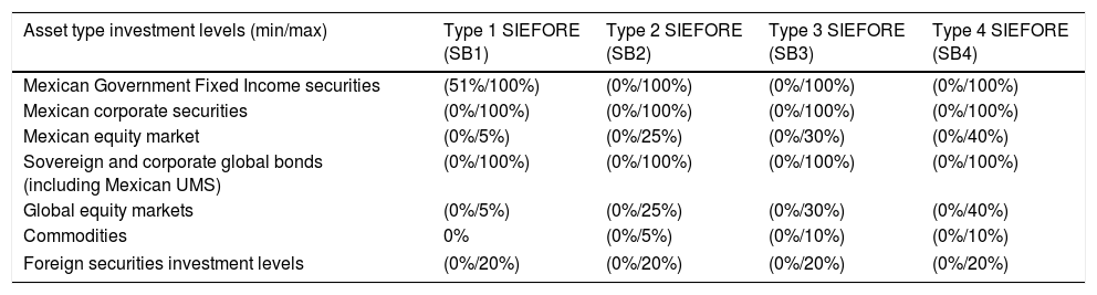
Since 1997, the Mexican pension fund system and its investment policy have been supervised by the regulatory authority: the CONSAR.⁴ At the beginning of this reformed pension system, the SIEFORES were allowed to invest only in Mexican Government Fixed Income securities. Since 2005, the system allowed to have two types of SIEFOREs. One for people with an age higher or equal to 56 years that invested in Fixed Income securities and a second one who invested at most the 15% of their portfolio in equities through structured notes. In March 2008 the CONSAR allowed the SIEFORES to work in a “life cycle” scheme where 5 type of SIEFOREs were managed with investment policy that allow to invest in Mexican and foreign securities, such as equities, real state investment trusts and commodities. Finally, in 2013 the five types of SIEFOREs were reduced to 4 with the investment policy given in Table 1.

Table 1.

The investment policy allowed by CONSAR.

Asset type investment levels (min/max)	Type 1 SIEFORE (SB1)	Type 2 SIEFORE (SB2)	Type 3 SIEFORE (SB3)	Type 4 SIEFORE (SB4)
Mexican Government Fixed Income securities	(51%/100%)	(0%/100%)	(0%/100%)	(0%/100%)
Mexican corporate securities	(0%/100%)	(0%/100%)	(0%/100%)	(0%/100%)
Mexican equity market	(0%/5%)	(0%/25%)	(0%/30%)	(0%/40%)
Sovereign and corporate global bonds (including Mexican UMS)	(0%/100%)	(0%/100%)	(0%/100%)	(0%/100%)
Global equity markets	(0%/5%)	(0%/25%)	(0%/30%)	(0%/40%)
Commodities	0%	(0%/5%)	(0%/10%)	(0%/10%)
Foreign securities investment levels	(0%/20%)	(0%/20%)	(0%/20%)	(0%/20%)

Source: CONSAR (2016a, 2016b).

As noted, the investment policy (since the beginning of the reform in 1997) suggested the presence or induction of a sort of “homogeneity” in the performance of the SIEFOREs that could translate into a lack of competitiveness. A first proof of this possibility is found with Guillén (2011) who made a Data Envelopment Analysis (DEA) and two OLS panel data regressions (one with fixed time effects and another one with fixed country effects) in pension funds from Mexico, Argentina, Bolivia, Colombia, Costa Rica, Chile, Peru, El Salvador and Uruguay. His results and conclusions motivate the present paper by the fact that even though the Mexican pension funds have an acceptable relation between their absolute and relative competitiveness, improvements must be made in Mexico and Latin America to enhance it. He observes also, as one of the causes of his findings, that the limited competitiveness gives no performance advantage to big pension funds even if they have a strong influence in the capital market by their size. This last result motivates our interest to check first if there is alpha generation in pension funds and then to check if the market share of the Mexican pension funds (SIEFOREs) is according to their alpha generation i.e. their good performance. Our rationale at the starting point of this paper was: “If we find no alpha generation a pension fund and homogeneity in its performance related to the one observed among competitors, we will find a cause for demand inelasticity as Calderón-Colín, Domínguez, and Schwartz (2009) suggest”.

Since the inception of this new pension system in Mexico, several studies have been made in order to test the historical origins of the aforementioned reform and also to tests the improvements that could be made to enhance the economic impact and welfare of pension savers. Among all these that will be mentioned in detail in the literature review section, we want to note the aforementioned one of Calderón-Colín et al. (2009) who found, as previously told, that the pension investment decision (i.e. the SIEFORE selection) is noisy and uninformed, leading to the concept of pension fund demand inelasticity that is the key concept that motivates this paper. With their results and tests, they observe that Mexican pension savers decide to invest in a pension fund (SIEFORE) not because it is among the best performers (in a return or risk-return profile); but by the influence of big marketing efforts or “institutional issues” like the fact that the selected SIEFORE is part of a big financial institution or an insurance company (suggesting “back to back” practices).

This last result is the one that inspires the current research along with the one of Guillén (2011). Here we want to check if there are SIEFOREs that outperform the other ones in the market by paying positive and statistically significant alpha against their investment style peers or against all the SIEFOREs (even against SIEFORES of other types managed by the same AFORE) in the market. If this is the case, these SIEFOREs should be the ones with the biggest market share. If we don’t find evidence of positive alphas, there would be proofs that the SIEFORES have homogeneous performance and therefore, there are no incentives to change of SIEFORE (i.e. an inelastic demand). Also if we find betas closer to 1 in the factor models that use the all SIEFORE system performance, there will be also proofs of performance homogeneity and a lack of competitive advantage among funds.

Once that we have presented our main research aim and given the previous work that motivates the present one, we structured the paper as follows: in the next section we describe the data selection and processing to test the homogeneity among SIEFORES and we also present our main findings. Finally we continue with our conclusions and our suggestions for further research in the subject.

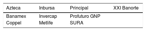
2

Methodology

2.1

Data processing

In order to test if there is homogeneity in the performance and also a cause of noisy investment decision in the Mexican pension funds, we will use the historical data of the price of the stock of each SIEFORE in each of the four SIEFORE types. By the fact that some of the SIEFOREs have merged with another ones we will use the historical daily price of the SIEFOREs shown in Table 2 from February 24, 2005 to November 30, 2016 in order to avoid survivor bias and time series with heterogeneous length.

Table 2.

List of SIEFORES in the sample.

Azteca	Inbursa	Principal	XXI Banorte
Banamex	Invercap	Profuturo GNP
Coppel	Metlife	SURA

Source: CONSAR (CONSAR, 2016a, 2016b).

Following this, we found in CONSAR (2016a, 2016b) the historical value of the performance index of each type of SIEFOREs and a performance benchmark calculated for all the SIEFOREs (or SIEFORE system). For the benchmarks of each SIEFORE type we denoted each type with the SB (SIEFORE Basic) letters and the type of SIEFORE: SB01, SB02, SB03 and SB04. For the benchmark of all the SIEFORES we simply labeled it as the “All” benchmark in our analysis. We decide to use these benchmarks, in contrast to De la Torre Torres et al. (2015a, 2015b) who use the minimum variance, the Max Sharpe or the target position portfolios. Our decision is based by the fact that these benchmarks, calculated and recently published by CONSAR (after De la Torre et al.) measure the net performance of the SIEFORES and not the theoretical portfolio. As previously stated, our first aim is to test the homogeneity in the observed results among SIEFORES instead of testing the performance of each of them against a theoretical portfolio. We also want to test if there is alpha generation in relation with other competitors i.e. we want to check how competitive is each SIEFORE in comparison to the other ones.

If there is positive alpha, then the SIEFORE could have taken more specific risk but, on exchange, they have generated significant positive alpha.

We also tested, in a second factor model, the performance of each SIEFORE of each type against “all” SIEFOREs (by using the “All” SIEFOREs benchmark) because this last benchmark incorporates the performance of all the pension funds in the system. We perform this last test because we want to go in line with Martínez and Venegas (2014) who found underperformance of the type 2 SIEFORES if they incorporate skewness and ARCH effects in the volatility. Finally we wanted to test, in a third model, each SIEFORE against both benchmarks (the SIEFORE type and the “All” one) to test if there is alpha generation by tacking into account the homogeneity given by the investment policy of each SIEFORE and to check, at the same time, if there is lack of alpha generation, given the potential homogeneity between SIEFORES in all the system.

In order to process the data we used the historical stock-market prices of the SIEFORES and the historical values of the benchmarks. With this data, we calculated their continuous-time price variation at time t with the next expression:

Once that we calculated these return values, we ran the three aforementioned factor models. The first one that explains the relation and influence of the SIEFORE type benchmark, the second one with the “All” benchmark and a third one with both benchmarks as stated in the next functional forms:

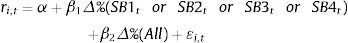
In the previous expressions, Δ % (SB1_tor SB2_tor SB3_tor SB4_t) is the continuous-time return of the SIEFORE type benchmark, Δ % (All) is the continuous-time return of the “all” SIEFOREs benchmark, β₁ and β₂ their corresponding sensitivities or systemic risk indicators⁵ and ¿_i,t is the residual or continuous-time variation attributed to unexplained factors in (2), (3) or (4).⁶

Once that we made these test, we calculated (3) in a recursive manner with data from February 24, 2005 as t₀ and an increasing monthly time window with T = February 28, 2006. With this recursive analysis we checked for the robustness of the alpha generation. We also observed historical values of p(α) and β₂. Once that our data-processing method is given, we will proceed to review the results, starting with type 1 SIEFOREs.

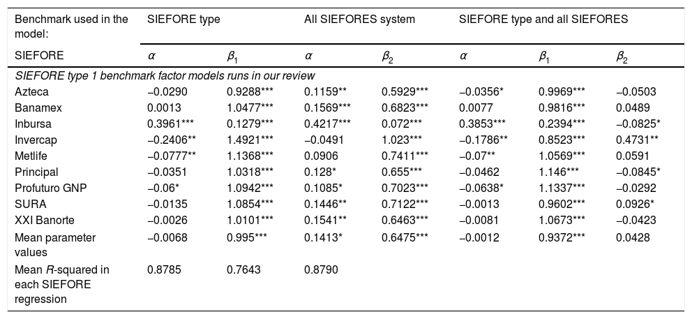
2.2

Data analysis

In Table 3 we present the results of the factor models made with (1)–(3) in type 1 SIEFORES. In different columns we show the values of α, β₁ and β₂ for each model, along with their respective probabilities or significance levels with asterisks.⁷ As noted, only two SIEFORES (Invercap and Metlife) had a significant but negative α. Also Inbursa shows a significant and positive value but, in general, its historic performance has been low compared with the performance of other SIEFORES, given a low beta of 0.1279. This last result is due to a possible lack of competitiveness in this specific case and a low attachment to the investment policy, as the R-squared value⁸ of 0.2937 suggest.

Therefore, with the exception of Inbursa who had a different performance and a lower volatility than all the studied SIEFORES, practically all the SIEFORES had a similar performance, suggesting a factual homogeneity in their behavior and a lack of alpha generation. This result shows that there is practically a similar performance in all the SIEFORES even if, in the short term, some SIEFORES show over-performance.

This sort of homogeneity can be advised in the β₁ values i.e. the β₁ values of each SIEFORE against their competitors. The mean value is 0.9950 with significant values surrounding 1. So if we find homogeneous values, we attribute this finding to a lack of incentive to enhance performance. So, the SIEFORES in this case are no competitive and the selection by investors could not be made by means of a good performance but due to other external and different factors than the return paid. A potential cause of this result could be the investment policy allowed by CONSAR.

An interesting result that we present in Table 3 is the mean values, especially in the two-factor model of (4). The value of the β₂ for the “all” SIEFORES index, is small and, in this type of SIEFORE, we found no evidence of homogeneity. As we will see in the next subsections for the other three types of SIEFOREs, the value of β₂ is getting closer to 1, and no alpha is generated, suggesting the presence of homogeneity in the performance of the pension funds. Also the R-Squared levels are much better with the “All” benchmark than with the specific SIEFORE type benchmark regression.

When we compare (in Table 4) the performance of each type 2 SIEFORE against its investment style benchmark (i.e. against its peers in the same type of SIEFORE with the same investment policy) we arrive to the same conclusion as in the type 1 SIEFORES: there is no positive alpha generation and, in the cases where the values of α are significant, the values of this parameter are negative. The only exception, as in the previous case, is Inbursa, given the lack of performance and a divergence from the investment policy. As we stated previously, an interesting feature are the values of β₂. For this type of SIEFOREs the values are close to 1 (the mean of β₂ for all these SIEFOREs is 0.944). This value suggests that even though the higher exposure to Mexican and international stocks is bigger than the previous SIEFORE type, there is an unexpected homogeneity in the performance of the pension funds, given the higher investment limit in stocks and commodities.⁹

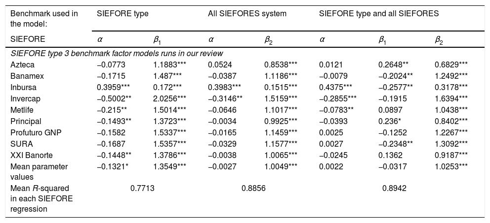
In the type 3 SIEFORES we found similar conclusions than the two previous ones but we want to observe that the values of β₁ in (3) and β₂ in (4) are also closer to 1 i.e. the influence of the “all” SIEFOREs benchmark is higher than the specific SIEFORE type one and two. Also the explanation of the regression (adjusted R-squared) tends to increase in the two models where the “All” SIEFORES benchmark is present. Another interesting finding is the fact that in the factor model with the two benchmarks, the specific type SIEFORE benchmark has a negative value in some funds and in five funds is not significant. That suggests us that the performance of almost all the funds is explained by “All” the SIEFORES in the market than by the SIEFORE type benchmark (i.e. investment policy). So, the fact of having more influence of the “All” SIEFORES instead of the specific type benchmark, along with zero or negative alpha generation, leads us to conclude (as previously stated) that there is either a lack of incentives to enhance performance given the uninformed and noisy decision by investors or there is an influence from the investment policy that induces the observed homogeneity. If the last case is true, then, the decision made by investors is still noisy and (more worrying) uninformed.

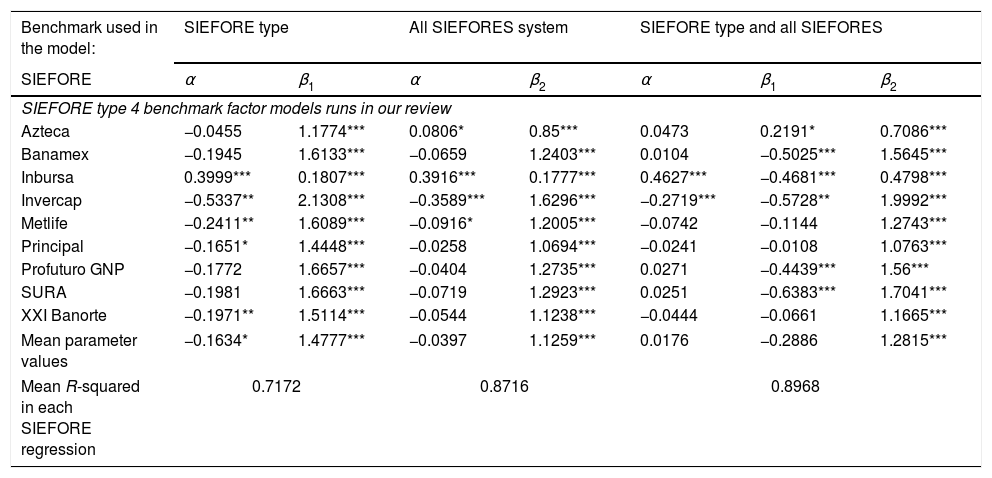
Finally we present the results for the type 4 SIEFORES in Table 6. We have similar performance conclusions than the previous SIEFORE types but now the influence of the “All” SIEFOREs is higher than 1 and the influence of the specific type SIEFORES is zero or negative. Why does this result arise? A possible explanation is the fact that the investment policy among the four types of SIEFORES is not as different as Table 1 suggest. More specifically speaking, a quick observation of the p-values of β₂ in Tables 3–6 suggest that only the benchmark that model the performance of “all” the SIEFORES in the system is the explanation for the performance of each SIEFORES e.g. SIEFORE A type 4 has a performance due to the performance of the financial markets allowed in the investment policy and not to management skills. Also the explanation could be extended to an investment policy in each SIEFORE type that allows similar investment proportions among SIEFORES, despite the fact of different investment limits.

Table 3.

Performance results of the type 1 SIEFOREs in the three factor models.

Benchmark used in the model:	SIEFORE type		All SIEFORES system		SIEFORE type and all SIEFORES
SIEFORE	α	β1	α	β2	α	β1	β2
SIEFORE type 1 benchmark factor models runs in our review
Azteca	−0.0290	0.9288***	0.1159**	0.5929***	−0.0356*	0.9969***	−0.0503
Banamex	0.0013	1.0477***	0.1569***	0.6823***	0.0077	0.9816***	0.0489
Inbursa	0.3961***	0.1279***	0.4217***	0.072***	0.3853***	0.2394***	−0.0825*
Invercap	−0.2406**	1.4921***	−0.0491	1.023***	−0.1786**	0.8523***	0.4731**
Metlife	−0.0777**	1.1368***	0.0906	0.7411***	−0.07**	1.0569***	0.0591
Principal	−0.0351	1.0318***	0.128*	0.655***	−0.0462	1.146***	−0.0845*
Profuturo GNP	−0.06*	1.0942***	0.1085*	0.7023***	−0.0638*	1.1337***	−0.0292
SURA	−0.0135	1.0854***	0.1446**	0.7122***	−0.0013	0.9602***	0.0926*
XXI Banorte	−0.0026	1.0101***	0.1541**	0.6463***	−0.0081	1.0673***	−0.0423
Mean parameter values	−0.0068	0.995***	0.1413*	0.6475***	−0.0012	0.9372***	0.0428
Mean R-squared in each SIEFORE regression	0.8785	0.7643	0.8790

Note: We denoted the parameter with c* if it is significant at a 10% probability level, c** if it is at a 5% level, and c*** if it is at 1%.

Source: Data from our analysis and SIEFOREs’ prices from CONSAR (2016a, 2016b).

Table 4.

Performance results of the type 2 SIEFOREs in the three factor models.

Benchmark used in the model:	SIEFORE type		All SIEFORES system		SIEFORE type and all SIEFORES
SIEFORE	α	β1	α	β2	α	β1	β2
SIEFORE type 2 benchmark factor models runs in our review
Azteca	−0.0497	1.0883***	0.0741*	0.7734***	0.0234	0.3333***	0.5583***
Banamex	−0.1201	1.3465***	0.0098	0.9967***	0.0113	−0.0104	1.0033***
Inbursa	0.3799***	0.161***	0.3912***	0.1264***	0.4031***	−0.0779	0.1767***
Invercap	−0.4226**	1.8577***	−0.2403**	1.3695***	−0.247***	0.0445	1.3408***
Metlife	−0.1768**	1.391***	−0.0296	1.0073***	−0.0639*	0.2259***	0.8615***
Principal	−0.1266**	1.2969***	0.0218	0.92***	−0.0411	0.4144***	0.6526***
Profuturo GNP	−0.1168	1.3901***	0.0189	1.026***	0.0159	0.0196	1.0134***
SURA	−0.1136	1.3725***	0.0157	1.0211***	0.0257	−0.0654	1.0633***
XXI Banorte	−0.0869	1.2543***	0.0509	0.8996***	0.0059	0.2961***	0.7086***
Mean parameter values	−0.0926	1.2398***	0.0347	0.9044***	0.0148	0.1311	0.8198***
Mean R-squared in each SIEFORE regression	0.7956		0.8814		0.8859

Note: We denoted the parameter with c* if it is significant at a 10% probability level, c** if it is at a 5% level, and c*** if it is at 1%.

Source: Data from our analysis and SIEFOREs’ prices from CONSAR (2016a, 2016b).

Table 5.

Performance results of the type 3 SIEFOREs in the three factor models.

Benchmark used in the model:	SIEFORE type		All SIEFORES system		SIEFORE type and all SIEFORES
SIEFORE	α	β1	α	β2	α	β1	β2
SIEFORE type 3 benchmark factor models runs in our review
Azteca	−0.0773	1.1883***	0.0524	0.8538***	0.0121	0.2648**	0.6829***
Banamex	−0.1715	1.487***	−0.0387	1.1186***	−0.0079	−0.2024**	1.2492***
Inbursa	0.3959***	0.172***	0.3983***	0.1515***	0.4375***	−0.2577**	0.3178***
Invercap	−0.5002**	2.0256***	−0.3146**	1.5159***	−0.2855***	−0.1915	1.6394***
Metlife	−0.215**	1.5014***	−0.0646	1.1017***	−0.0783**	0.0897	1.0438***
Principal	−0.1493**	1.3723***	−0.0034	0.9925***	−0.0393	0.236*	0.8402***
Profuturo GNP	−0.1582	1.5337***	−0.0165	1.1459***	0.0025	−0.1252	1.2267***
SURA	−0.1687	1.5357***	−0.0329	1.1577***	0.0027	−0.2348**	1.3092***
XXI Banorte	−0.1448**	1.3786***	−0.0038	1.0065***	−0.0245	0.1362	0.9187***
Mean parameter values	−0.1321*	1.3549***	−0.0027	1.0049***	0.0022	−0.0317	1.0253***
Mean R-squared in each SIEFORE regression	0.7713		0.8856		0.8942

Note: We denoted the parameter with c* if it is significant at a 10% probability level, c** if it is at a 5% level, and c*** if it is at 1%.

Source: Data from our analysis and SIEFOREs’ prices from CONSAR (2016a, 2016b).

Table 6.

Performance results of the type 4 SIEFOREs in the three factor models.

Benchmark used in the model:	SIEFORE type		All SIEFORES system		SIEFORE type and all SIEFORES
SIEFORE	α	β1	α	β2	α	β1	β2
SIEFORE type 4 benchmark factor models runs in our review
Azteca	−0.0455	1.1774***	0.0806*	0.85***	0.0473	0.2191*	0.7086***
Banamex	−0.1945	1.6133***	−0.0659	1.2403***	0.0104	−0.5025***	1.5645***
Inbursa	0.3999***	0.1807***	0.3916***	0.1777***	0.4627***	−0.4681***	0.4798***
Invercap	−0.5337**	2.1308***	−0.3589***	1.6296***	−0.2719***	−0.5728**	1.9992***
Metlife	−0.2411**	1.6089***	−0.0916*	1.2005***	−0.0742	−0.1144	1.2743***
Principal	−0.1651*	1.4448***	−0.0258	1.0694***	−0.0241	−0.0108	1.0763***
Profuturo GNP	−0.1772	1.6657***	−0.0404	1.2735***	0.0271	−0.4439***	1.56***
SURA	−0.1981	1.6663***	−0.0719	1.2923***	0.0251	−0.6383***	1.7041***
XXI Banorte	−0.1971**	1.5114***	−0.0544	1.1238***	−0.0444	−0.0661	1.1665***
Mean parameter values	−0.1634*	1.4777***	−0.0397	1.1259***	0.0176	−0.2886	1.2815***
Mean R-squared in each SIEFORE regression	0.7172		0.8716		0.8968

Note: We denoted the parameter with c* if it is significant at a 10% probability level, c** if it is at a 5% level, and c*** if it is at 1%.

Source: Data from our analysis and SIEFOREs’ prices from CONSAR (2016a, 2016b).

A strong proof of this statement is, again, the p-values of β₁ and β₂. In Table 3 (related to SIEFORES type 1, the most conservative of the four types), it is noted that β₂ is not statistically significant or different from zero in all the SIEFORES but this situation changes gradually from SIEFORES type 2 to SIEFORES type 4 (Tables 4–6). In those tables, the p-values of β₂ are significant, suggesting us that the performance of the SIEFORES of this type is not different from the other types. This lead us to observe that the aforementioned theoretical SIEFORE A type 4 has practically the same performance than the SIEFORE A types 1, 2 and 3, by the fact that the funds are managed by the same asset manager A with a general or “official” investment policy.

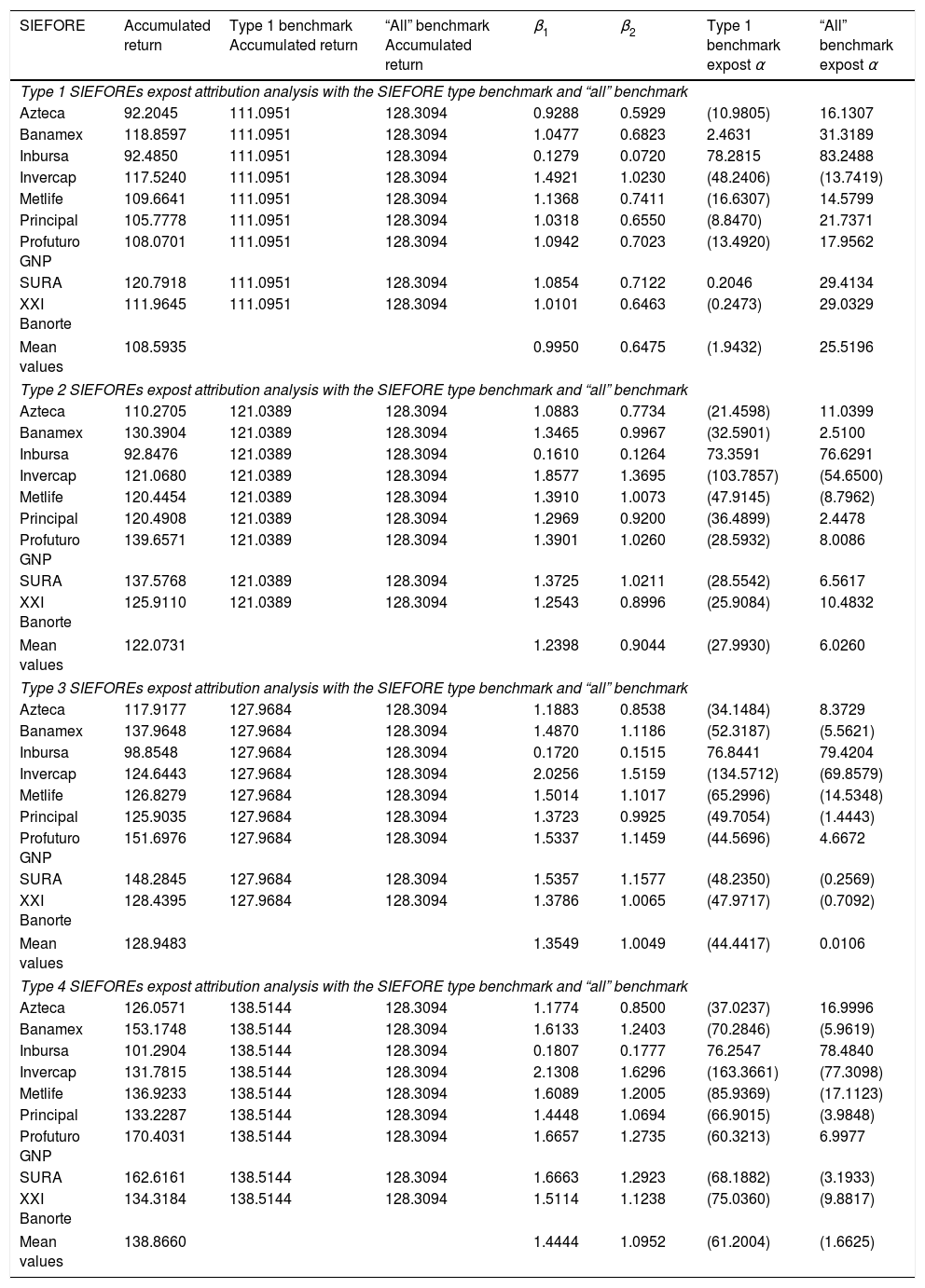
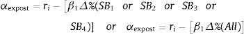
With this observed result and with all the studies presented here, we found evidence that suggest “homogeneity” in the performance of SIEFORES in Mexico. One of the potential counter-arguments to our review is that the alpha generation should be expressed in terms of the observed return or turnover in the SIEFORE (r_i) related with the β₁ of that SIEFORE and the observed turnover or return in the SIEFORE type benchmark or the “All” benchmark by following this expression of an ex-post Jensen's alpha:

In order to answer this question, we present the results of the alpha generated by each SIEFORE given (5) in Table 7. The last two columns show, respectively, the alpha generation in each SIEFORE against the turnover of the SIEFORE type benchmark in model (2) and also against the “All” benchmark in model (3). As expected, the generation of alpha (ex-post alpha) is negative in almost all the SIEFORES for the type 1 group and starts to increase in type 4 SIEFOREs i.e. even though the SIEFORES paid a higher nominal turnover, their theoretical expected value given β_i in each model is higher than the observed one.

Table 7.

Corollary of β results and ex-post alpha generation.

SIEFORE	Accumulated return	Type 1 benchmark Accumulated return	“All” benchmark Accumulated return	β1	β2	Type 1 benchmark expost α	“All” benchmark expost α
Type 1 SIEFOREs expost attribution analysis with the SIEFORE type benchmark and “all” benchmark
Azteca	92.2045	111.0951	128.3094	0.9288	0.5929	(10.9805)	16.1307
Banamex	118.8597	111.0951	128.3094	1.0477	0.6823	2.4631	31.3189
Inbursa	92.4850	111.0951	128.3094	0.1279	0.0720	78.2815	83.2488
Invercap	117.5240	111.0951	128.3094	1.4921	1.0230	(48.2406)	(13.7419)
Metlife	109.6641	111.0951	128.3094	1.1368	0.7411	(16.6307)	14.5799
Principal	105.7778	111.0951	128.3094	1.0318	0.6550	(8.8470)	21.7371
Profuturo GNP	108.0701	111.0951	128.3094	1.0942	0.7023	(13.4920)	17.9562
SURA	120.7918	111.0951	128.3094	1.0854	0.7122	0.2046	29.4134
XXI Banorte	111.9645	111.0951	128.3094	1.0101	0.6463	(0.2473)	29.0329
Mean values	108.5935			0.9950	0.6475	(1.9432)	25.5196
Type 2 SIEFOREs expost attribution analysis with the SIEFORE type benchmark and “all” benchmark
Azteca	110.2705	121.0389	128.3094	1.0883	0.7734	(21.4598)	11.0399
Banamex	130.3904	121.0389	128.3094	1.3465	0.9967	(32.5901)	2.5100
Inbursa	92.8476	121.0389	128.3094	0.1610	0.1264	73.3591	76.6291
Invercap	121.0680	121.0389	128.3094	1.8577	1.3695	(103.7857)	(54.6500)
Metlife	120.4454	121.0389	128.3094	1.3910	1.0073	(47.9145)	(8.7962)
Principal	120.4908	121.0389	128.3094	1.2969	0.9200	(36.4899)	2.4478
Profuturo GNP	139.6571	121.0389	128.3094	1.3901	1.0260	(28.5932)	8.0086
SURA	137.5768	121.0389	128.3094	1.3725	1.0211	(28.5542)	6.5617
XXI Banorte	125.9110	121.0389	128.3094	1.2543	0.8996	(25.9084)	10.4832
Mean values	122.0731			1.2398	0.9044	(27.9930)	6.0260
Type 3 SIEFOREs expost attribution analysis with the SIEFORE type benchmark and “all” benchmark
Azteca	117.9177	127.9684	128.3094	1.1883	0.8538	(34.1484)	8.3729
Banamex	137.9648	127.9684	128.3094	1.4870	1.1186	(52.3187)	(5.5621)
Inbursa	98.8548	127.9684	128.3094	0.1720	0.1515	76.8441	79.4204
Invercap	124.6443	127.9684	128.3094	2.0256	1.5159	(134.5712)	(69.8579)
Metlife	126.8279	127.9684	128.3094	1.5014	1.1017	(65.2996)	(14.5348)
Principal	125.9035	127.9684	128.3094	1.3723	0.9925	(49.7054)	(1.4443)
Profuturo GNP	151.6976	127.9684	128.3094	1.5337	1.1459	(44.5696)	4.6672
SURA	148.2845	127.9684	128.3094	1.5357	1.1577	(48.2350)	(0.2569)
XXI Banorte	128.4395	127.9684	128.3094	1.3786	1.0065	(47.9717)	(0.7092)
Mean values	128.9483			1.3549	1.0049	(44.4417)	0.0106
Type 4 SIEFOREs expost attribution analysis with the SIEFORE type benchmark and “all” benchmark
Azteca	126.0571	138.5144	128.3094	1.1774	0.8500	(37.0237)	16.9996
Banamex	153.1748	138.5144	128.3094	1.6133	1.2403	(70.2846)	(5.9619)
Inbursa	101.2904	138.5144	128.3094	0.1807	0.1777	76.2547	78.4840
Invercap	131.7815	138.5144	128.3094	2.1308	1.6296	(163.3661)	(77.3098)
Metlife	136.9233	138.5144	128.3094	1.6089	1.2005	(85.9369)	(17.1123)
Principal	133.2287	138.5144	128.3094	1.4448	1.0694	(66.9015)	(3.9848)
Profuturo GNP	170.4031	138.5144	128.3094	1.6657	1.2735	(60.3213)	6.9977
SURA	162.6161	138.5144	128.3094	1.6663	1.2923	(68.1882)	(3.1933)
XXI Banorte	134.3184	138.5144	128.3094	1.5114	1.1238	(75.0360)	(9.8817)
Mean values	138.8660			1.4444	1.0952	(61.2004)	(1.6625)

Source: Data from our analysis and SIEFOREs’ prices from CONSAR (2016a, 2016b).

3

Conclusions

The competitiveness of public pension funds, especially those who fit in the “Defined contribution” plan classification, is a very important issue that must be taken into account nowadays. The main reason of it is the fact that a higher return paid to investors will lead to a better pension at retirement. A better income for retired people will lead to a sustainable consumption and GDP creation, given the changing population conditions and the increase of the mean dead age in almost all the countries. In order to give more guidelines of the necessary tasks needed to enhance pension plans (specifically in the Mexican case), we have followed the line opened by Calderón-Colín et al. (2009) and Guillén (2011) who study the informational efficiency in the pension fund selection (the former) and the competitiveness of these to generate value to investors (the latter). We made a performance attribution test in order to detect if there is a connection between the performance and the decision making process that is “noisy and uniformed” as Calderón-Colín et al. (2009) prove.

One of the first places that we suggest as a potential cause of this last result is the official or allowed public investment policy for all the SIEFORES in Mexico. We state this by the homogeneity in the performance that we found in all the SIEFORES even if they have different life-cycle investment restrictions (the Mexican public pension funds or SIEFOREs are public funds that work as life-cycle mutual funds). We suspect that the investment policy generates homogeneity in the performance not only in the SIEFORES of similar life-cycle (risk-return) type but also between SIEFORES among different ones. Our rationale is that there should be performance heterogeneity between SIEFORES of the same type and also among SIEFOREs of different groups or types in the presence of real competition between funds. If this rationale holds the individual investment decision should not be made based in the performance of the pension fund and not with the influence of external factors such as the ones suggested by Calderón-Colín et al. (2009).

On the other hand, if there is (statistically significant) alpha generation in the long term, there could be a window to enhance competitiveness and, as a consequence, the performance or return paid to pension savers.

By using data of 10 SIEFOREs from March 2005 to November 2016 we tested our rationale and found that there is no alpha generation if we compare the performance of each SIEFORE with their group or peer type benchmark. We also found this if we test the same performance against a portfolio or benchmark composed of all the SIEFORES in the Mexican pension fund system. An interesting finding for us is the fact that the beta of each SIEFORE against the “all” SIEFOREs benchmark is practically of 1 in almost all the tested funds.

We also found that the different risk and investment limits of the investment policy in each SIEFORE type do not produce heterogeneity in the performance of the tested funds.

This result is useful by the fact that CONSAR (the Mexican regulatory pension fund) has allowed in 2017 (the moment that this paper was written) to have a “diversified” pension portfolio that could include SIEFORES from the same fund manager but with different types. This “portfolio decision” can be done freely each three years by pension savers.

The results of this paper suggest that this sort of life-cycle diversification could lead to marginal improvements in the performance of pension savers if they have a diversified portfolio with not only different type of SIEFORES but also with different funds. This last statement, even though is an actual one (specially for the Mexican case) it must be tested given the evidence presented in this paper. Therefore we suggest, as future research guideline, to check the benefit of a diversified portfolio with different SIEFORES for Mexican pension fund savers, against the actual “single SIEFORE choice scenario”. Why? Because if there is strong evidence of over-performance and mean-variance efficiency improvements with this diversified strategy, it will be thanks to an induced heterogeneous performance of the more diversified simulated portfolio. If the results show no improvements in the performance it will be due to the investment policy that leads to a portfolio with assets that have practically the same performance among them.