Determinants of the spending of sporting tourists: The case of attendees at professional basketball

Abstract

This article analyses the determinants of attendees’ tourism spending at professional basketball matches during the 2012/2013 season. For this purpose, it applies a linear quantile regression and considers the effect of specific sports event variables which have rarely been assessed in this type of study. Empirical results confirm that the determinants of expenditure have a different influence depending on the spending level. Individual spending is principally influenced by the origin of the attendees as well as by several other sports factors such as the time the match takes place, the admission price, or the sporting level of the rival team. The study establishes two levels of spending to identify the different behaviors that correspond to each of the factors under study. The findings could provide a useful input into tourism strategies related to the hosting of sport events.

1

Introduction

The analysis of the individual spending behavior of visitors to specific destinations is increasingly becoming a topic of interest, according to Brida, Disegna, and Osti (2013), Craggs and Schofield (2009), Dolnicar et al. (2008), Hung, Shang, and Wang (2012) and Nicolau and Más (2005). Tourism demand is mainly analyzed using a macro approach, in which the unit of analysis is a set of aggregated data. These kinds of studies use economic indicators such as the influence of the tourism sector on GDP, GVA or employment at the national or regional level. Individual spending behavior and the sociodemographic and economic factors that affect spending patterns (i.e., the micro approach) have been studied to a lesser extent (Brida et al., 2013; Fredman, 2008; Laesser & Crouch, 2006).

Reviews of the previous literature on tourism demand including the works of Lim (1997, 2006) and Crouch (1994) reflect that there is a lack of studies employing micro-economic analysis. Lim (2006) explains that only 8 out of the 124 articles studied employed this type of analysis. Wang and Davidson (2010) indicate that the first studies concerning demand at a micro level were carried out by Mak, Moncur, and Yonamine (1977). Subsequently, this type of work aroused the interest of researchers once again in the 1990s. As of then, interest increased rapidly, especially at the turn of the century.

In the case of sports tourism, the same situation is observed. Studies have neglected the specific aspects of products and services and have focused on economic impact and the use of aggregated data. It therefore now seems reasonable to also focus on understanding the spending behavior of sports tourists who come as spectators (Brida, Schubert, Osti, & Barquet 2011; Cannon & Ford, 2002; Yusof, Shah, & Geok, 2012) and participants (Dixon, Backman, Backman, & Norman, 2012; Downward, Lumsdon, & Weston, 2009; Gibson, 2005).

Mok and Iverson (2000) explain that the growth of international tourism and tourist spending has extended the interest in carrying out research on consumer behavior. Understanding the patterns and activities of tourist spending when visiting a particular destination is a key issue in strategic facility planning. Knowing the factors influencing tourist behavior can lead to the better planning of marketing and sales management and improved industry opportunities (Laesser & Crouch, 2006; Oh, Cheng, Lehto, & O’Leary, 2004; Saayman & Saayman, 2009; Saayman & Saayman, 2012).

In light of the above, this paper aims to identify the factors influencing the expenditure of those attending the matches of a top-level professional league basketball team. The team Rio Natura Monbus Obradoiro (commonly known as Obradoiro), which plays in the top Spanish league (Liga Endesa), was taken as the case example for this study. The Liga Endesa is Spain's professional basketball league. It is a relevant sporting event that has gained both national and international importance. It consists of 17 teams that regularly compete. The top eight finishers at the end of the regular season face a second round of play-offs, after which the League champion is proclaimed. The paper additionally analyses the existence of differences in the spending behavior pattern of attendees according to how much they spend.

The contribution of this work lies in the way it analyses the determinants of spending for a type of sporting event that, as yet, has not been discussed in the literature (for a professional team over a whole season). This kind of empirical study is becoming increasingly relevant, given that leagues differ from occasional events (which have been more widely studied). Events that take place every season are capable of attracting attendees to the territory regularly. Besides, attendees often repeat their visit throughout the season. It is thus increasingly important to collect reliable information about attendee spending behavior. Event organizers will be better equipped to attract attendees end develop their loyalty, while policy makers could use the results to help maximize the spending impact on the local economy. Another contribution of this work rests on the use of sports factors in addition to factors most commonly employed in previous models: sociodemographic, economic and tourist variables.

The paper is organized as follows. The next section presents the literature review relating to expenditure behaviors in tourism and sport events. This is followed by a description of the sample and variables used in the empirical analysis, before an explanation of the methodology. The fifth section presents the results, with the final sections containing the discussion and conclusions.

2

Literature review

The studies on tourist spending behavior by Brida and Scuderi (2013), Lehto, O’Leary, and Morrison (2002) and Wang, Rompf, Severt, and Peerapatdit (2006) affirm that economic and sociodemographic variables, as well as characteristics related to travel, are the most frequently used in studies on spending determinants. As these works explain, they use economic variables such as income, assets or the existence of economic difficulties. In terms of the sociodemographic variables, current models have used age, education, sex, marital status, residence, occupation or profession and race. For their part, travel characteristics are usually represented by accommodation, length of stay, activities undertaken during the trip, destinations visited, source of travel information, transportation, purpose for traveling, previous experience at the destination or group size (Brida & Scuderi, 2013; Wang & Davidson, 2010).

Specifically, studies of the determinants of spending at sporting events have constructed models for analysis from a combination of socioeconomic variables and the demographic characteristics. Every sporting event is observed to have different characteristics influencing the choice of variables used to build the model. Bilgic, Florkowski, Yoder, and Schreiner (2008), Taks, Green, Chalip, Kesenne, and Martyn (2013) and Downward et al. (2009) have analyzed participant spending. Meanwhile, Yusof et al. (2012), Brida et al. (2011) and Cannon and Ford (2002) have focused on spectator spending.

In relation to economic factors, Brida and Scuderi (2013) and Wang and Davidson (2010) explain, individual income is one of the most important and commonly used determinants in these types of studies. Yet, respondents are more reluctant to share this type of data. Thus, in cases where it is not possible to obtain personal income for the dataset, other variables are used to represent the level of income. Abbruzzo, Brida, and Scuderi (2014), Aguiló Perez and Juaneda (2000), Medina-Muñoz and Medina-Muñoz (2012) and Svensson, Moreno, and Martín (2011) employ variables such as occupation and/or profession to represent the level of income.

Taking into consideration other kind of factors, Abbruzzo et al. (2014) explain that, it is interesting to consider the variable of other activities, that is, if attendee performs other activities besides attending the event, such as, tourism, shopping or leisure activities. The objective of this variable is to identify whether there are activities that are contributing to increase attendee spending in the geographic area where the study is taking place. Another case is represented by variables that characterize the event. Authors such as Bilgic et al. (2008), Dixon et al. (2012), Shani, Wang, Hutchinson, and Lai (2010) and Sato, Jordan, Kaplanidou, and Funk (2014) include this kind of variables. However, most papers do not do this.

Economic and sociodemographic attributes are insufficient to understand decisions concerning tourist destination. Therefore, the use of psychographic variables is proposed to justify decisions regarding tourism destination development (Lehto et al., 2002; Wang et al., 2006). Psychographic variables include all of the characteristics that may influence consumer response to products and services (Lehto et al., 2002) such as interests, opinions, attitudes and lifestyles (Brida & Scuderi, 2013). Thrane (2002), Chen and Chang (2012), Henthorne (2000), Aguiló Perez and Juaneda (2000) and Abbruzzo et al. (2014) include psychographic variables when studying the determinants of expenditure. Psychographic variables have proven to be powerful predictors of travellers’ decisions in tourist destinations (Lehto, Morrison, & O’Leary, 2001; Lehto et al., 2002) and, by association, they can also contribute to a better understanding of spending patterns (Wang et al., 2006).

Metric and categorical response models are used to study the determinants of cost models. In the former, the most common method is the classical linear regression model by ordinary least squares (OLS). The most usual alternative estimation procedures to the OLS are Tobit regression model, Double-Hurdle Model and the Negative Binomial Model (Brida & Scuderi, 2013). Other alternative to OLS model is the quantile regression approach which makes possible to assess local behavior in specific portions of the empirical distribution according to the different quantiles rather than the mean values. The universal Logit, Probit and Logit ordinal models are among the categorical response models (Brida & Scuderi, 2013).

In the case of sports tourism, there are studies that identify the determinants of event attendance using quantile regression. This is the case of papers by Jane, Kuo, Wu, and Chen (2010), that it investigates the determinants of game-day attendance in the Chinese Professional Baseball League (CPBL) from 2001 to 2007. Other example is the paper by Serrano, García-Bernal, Fernández-Olmos, and Espitia-Escuer (2015). It focuses on the relationship between the expected quality of the event and attendance at the European football stadiums. Both works found that the outcome uncertainty and the quality of the contestant teams have positive effect on attendance demand. However, no studies have been conducted using quantile regression to analyze the spending patterns of those attending a sporting event. This study addresses this issue by providing evidence concerning the influence of a variety of proposed factors on different spending levels.

3

Data and variables

The data is derived from a survey of attendees at Obradoiro matches. A total of 2797 surveys were conducted at 11 of the team's 17 home matches during the 2012/2013 season and at the play-off game. Non-residents account for 64% of the sample, while residents account for 36%.

The survey was conducted on attendants with residence in the city of Santiago de Compostela (where the event takes place) as well as non-residents in the city. To ensure the randomness of the sample, interviewers followed a pattern of conduct addressing one out of every three persons (but only one person per group) in each area of the venue during different moments throughout the event. Nevertheless, this study only used data from the non-resident attendants whose sole purpose for traveling to the city was to attend the basketball match. The definition of economic impact indicates that only this type of attendee injects cash into the territory (Preuss, Könecke, & Schütte, 2010). Preliminary works on spending determinants have followed the same premise. Such is also the case of Dixon et al. (2012) and Sato et al. (2014).

The dependent variable is measured by the average individual expenditure per match attendant (only for non-residents). Attendee expenditure refers the total spending by each visitor in of Santiago de Compostela. It includes accommodation, food, shopping, leisure and other expenses. Attendee expenditure does not include transport expenditure to Santiago de Compostela from their city of origin. The surveyor first asks about the different expenditure items. If the answers are partial or null, the surveyor enquires about aggregate spending. If the respondents do not give a figure, they are asked to choose from one of the proposed intervals (less than 50€, 51€–100€, 101€–200€, 201€–300€, 301€–400€, 401€–500€ or over 500€). The average individual spending of the attendees is obtained from the data provided. The distribution of expenditure is normalized using its natural logarithm.

Expenditure on tickets (admission fees) is computed from the information provided by the event organizers. Attendees have not been asked about the money spent on tickets. In order to know a particular attendee's total expenditure, the average price of the ticket for each match has been added to the rest of the expenses. Ticket price varies from match to match.

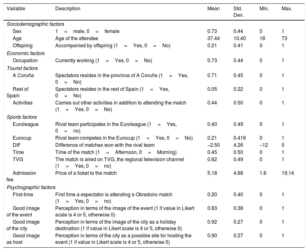
The explanatory variables are classified into sociodemographic, economic, tourist, psychographic and sports factors. A list and description of these variables are introduced in Table 1. The sociodemographic factors employed are age, gender and offspring. According to Wang and Davidson (2010), there are no common empirical findings concerning the effect of sociodemographic variables. Existing studies are very diverse and use different units of analysis. Marrocu, Paci, and Zara (2015) use sociodemographic variables, such as gender, as control variables in their empirical models.

Table 1.

List of explanatory variables.

Variable	Description	Mean	Std. Dev.	Min.	Max.
Sociodemographic factors
Sex	1 = male, 0 = female	0.73	0.44	0	1
Age	Age of the attendee	37.44	10.40	18	73
Offspring	Accompanied by offspring (1 = Yes, 0 = No)	0.21	0.41	0	1
Economic factors
Occupation	Currently working (1 = Yes, 0 = No)	0.73	0.44	0	1
Tourist factors
A Coruña	Spectators resides in the province of A Coruña (1 = Yes, 0 = No)	0.71	0.45	0	1
Rest of Spain	Spectators resides in the rest of Spain (1 = Yes, 0 = No)	0.05	0.22	0	1
Activities	Carries out other activities in addition to attending the match (1 = Yes, 0 = No)	0.44	0.50	0	1
Sports factors
Euroleague	Rival team participates in the Euroleague (1 = Yes, 0 = no)	0.40	0.49	0	1
Eurocup	Rival team competes in the Eurocup (1 = Yes, 0 = No)	0.21	0.416	0	1
DIF	Difference of matches won with the rival team	−2.50	4.26	−12	5
Time	Time of the match (1 = Afternoon, 0 = Morning)	0.45	0.50	0	1
TVG	The match is aired on TVG, the regional television channel (1 = Yes, 0 = no)	0.62	0.49	0	1
Admission fee	Price of a ticket to the match	5.18	4.68	1.6	19.14
Psychographic factors
First-time	First time a espectator is attending a Obradoiro match (1 = Yes, 0 = no)	0.20	0.40	0	1
Good image of the event	Perception in terms of the image of the event (1 if value in Likert scale is 4 or 5, otherwise 0)	0.83	0.38	0	1
Good image of the city	Perception in terms of the image of the city as a holiday destination (1 if value in Likert scale is 4 or 5, otherwise 0)	0.92	0.27	0	1
Good image as host	Perception in terms of the city as a possible site for hosting the event (1 if value in Likert scale is 4 or 5, otherwise 0)	0.90	0.27	0	1

The variable offspring is defined as a dummy variable indicating whether attendants are accompanied by their children. The survey is only addressed to people over 18 years of age. It considers that people who travel with their children take on their expenses. In studies of determinants of spending at tourist destinations, this variable usually refers to the number of household members or the number of minors (Brida & Scuderi, 2013). Here, this variable indicates that spectators have traveled to the match accompanied by their children. This data is more significant for the study, given that a person may have children and not take them along to the match.

Economic factors are measured by a categorical variable indicating whether the individual is employed or unemployed. The personal income of the attendants is not available in dataset. In this way, an alternative variable is used such as occupation. Regarding tourist factors, the origin of those attending and those undertaking other activities in the city in addition to attending the match (dummy variable) are included. In this paper, the origin of the attendees is classified into attendees from the rest of the province of A Coruña, the rest of Galicia and the rest of Spain.

A set of psychographic variables is proposed in order to check the extent to which they can explain the spending behavior of individuals attending a match. The set of psychographic variables consists of a dummy variable considering whether the espectator is attending the match for the first time or is repeating their attendance. In addition, three Likert scale variables express the attendee's assessment of the event, the city and the site of the venue (1 = very negative to 5 = very positive). We have created three dummy variables from these Likert type variables. They reflect if the image of the city, the event or the city as host is good (when the value in the response in the Likert scale is 4 or 5). These variables are those that we include in the model.

Finally, we consider a number of factors related to the type of event. Specifically, for this study, variables such as rival team, difference of matches won with the rival team, time of the match, broadcast on TV and price of the ticket have been included.

Certain characteristics of the event under study can influence attendee spending. The match schedule is not always the same. Matches may be held in the morning or afternoon. Similarly, the admission price varies depending on the type of match and the opponents. These data have been computed from the total ticket revenue and the attendants at each match. Thus, it is interesting to know how both variables influence individual attendee spending.

The variables Euroleague and Eurocup, which define whether the rival team usually plays in the Euroleague or the Eurocup, reflect the sporting level of the opponent team. The variable DIF represents the difference in matches won previously in the season with the opposing team. This figure is estimated by deducting the number of matches won by the away team from the matches won by Obradoiro at that time in the season (it can take positive and negative values). The variable TVG represents the matches broadcast by the regional television channel, Galician Television.

These variables seem to have an obvious influence on attendance. If the opposing team is at the top of the league table, if there is little difference between the teams in terms of points or if it is a game not being aired on TV, it seems reasonable to think that these factors will incentivize attendance. Although their influence on individual spending does not seem to be so perceptible, these variables affect the attendance of non-regular viewers (who are attracted by the opponent or the competitiveness of the game) whose spending behavior may differ from that of regular attendees. The significant effect of sports factors can be explained by the intangible effect generated by the attraction of spectators who are not regular viewers, who may take advantage of their visit to carry out other activities such as cultural tourism and shopping. Quick (2000) explains that attendees at sporting events are not homogeneous. Therefore, it has become increasingly relevant to identify how these variables affect the spending behavior of attendees.

4

Methodology

The determinants of expenditure are analyzed by estimating an OLS model and a quantile regression model. The first econometric tool is useful for detecting the central tendency of the data. It estimates the average spending response of those attending matches, to changes in the independent variables. The second analysis estimates the response in specific levels of spending; thereby, it identifies differences in the spending patterns of spectators according to how much they spend.

Ever since the seminal work of Koenker and Basset (1978) explaining its different scientific functionalities, quantile regression has been used to analyze determinants in different areas, including the economy and tourism. The work developed by Buchinsky (1994) is an example that applies quantile regression to study the wage structure of the United States in the period 1963–1987. A more recent paper by Koenker and Hallock (2001) explains the use of quantile regression in different areas and empirical works. Several authors emphasize that the additional information it provides facilitates understanding and explains tourist spending patterns (Chen & Chang, 2012; Hung et al., 2012; Lew & Ng, 2012; Marrocu et al., 2015), therefore making it suitable for analysing spending determinants.

As explained by Marrocu et al. (2015), when there is significant heterogeneity in the effects of variables, quantile regression is expected to provide a more complete picture of spending behavior, given that the effect of the explanatory variables can be observed across the entire distribution. Attendance at basketball matches involves a common minimum expense associated with the payment of an admission fee. From this expense, it can be produced expenses in accommodation, restaurant or shopping that depends on the different activities carried out by the assistant in Santiago de Compostela. Thus, a quantile regression provides additional information on the key factors influencing spending and reveals the marginal effects of the explanatory variables for different quantiles of tourism expenditure.

This paper analyses the expenditure of match attendees. This expenditure is no censored because there are no restrictions. It is different when the dependent variable is the demand for tickets (attendance), where some observations may be censored. On the other hand, the population under study here is people attending the matches. Those attending each match are random samples, because everybody wanting to attend the match can do so due to the fact that none of the matches were sold out. In that sense, there is no problem of selection bias.

The OLS model is formulated as follows:

where Y is the individual expenditure per match attendee. It is transformed through its natural logarithm in order to make it closer to the normal distribution. X is defined as the set of independent variables. X is represented by the vectors E, SD, S, T and PS:

• -

  E: economic variables

• -

  SD: sociodemographic variables

• -

  S: sports variables

• -

  T: tourist variables

• -

  PS: psychographic variables

The model is expressed as follows:

where LOGEXP_i is the total expenditure per assistant log transformed. The different β_i correspond to the estimated coefficients of the explanatory variables, i is the ith element (i > 0) and ¿_i corresponds to the error term with zero mean.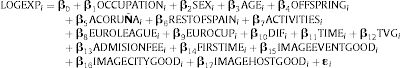

The quantile regression developed by Koenker and Basset (1978) seeks to model the relationship between X and Y for different quantiles of the distribution of the dependent variable Y.

where Y is the individual expenditure per match attendee. X is defined as the set of independent variables. β_i are the k coefficients of the quantile regression. τ is the weight of the positive residues and (1 − τ) is the weight of the negative residues.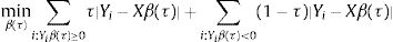

The estimation of the parameters, in the case of the quantile regression, is performed by minimizing weighted absolute deviations with asymmetrical weights. In this case, the dependent variable Y_i is represented – as it was in the linear regression – by the average individual expenditure of match attendees. Y_i is transformed through its natural logarithm. The variables E_i, SD_i, S_i, T_i and PS_i represent the set of independent variables (X_i) listed in the previous section.

“One of the main advantages of a quantile regression as opposed to an OLS is the use of deviations in absolute values rather than the squared deviations to estimate the parameters β_i. The estimates provided by the quantile regression are substantially unaltered by extreme values given that it ‘penalizes’ errors linearly; whereas, the OLS regression gives greater importance to raising errors to the square.” (Vicéns & Sánchez, 2012, p. 8).

In the validation of the model, the greatest advantage of quantile regression becomes its greatest drawback. There are no hypotheses concerning the error term, so the matrix of the variances and covariances of the estimators required to contrast significance is unknown. Standard errors and confidence limits for the estimates of quantile regression coefficients can be obtained using asymptotic and bootstrapping methods (Despa, 2012). Although both of these methods provide robust results, bootstrapping achieves the best results (Chasco & Sánchez, 2012; Gould, 1997; Hao & Naiman, 2007; Vicéns and Sánchez, 2012). Bootstrapping requires the use of an appropriate statistics program. STATA has been used to perform the estimations.

Using the bootstrap technique allowed us to obtain the variance and covariance matrix of the estimators, therefore permitting to test the hypotheses. The hypotheses are based on checking whether the quantiles are the same or whether there are significant differences among them. Interquantile regression is used to contrast these hypotheses. Interquartile regression allows to check if there are significant differences among quantiles. Therefore, a different behavior among the factors regarding the dependent variable is revealed. According to Marrocu et al. (2015), equality tests provide a more rigorous assessment of quantile regression results because they help to identify whether the differences between coefficients are related to significant changes in the behavior of tourists, or whether they are due to the variability of the sample.

5

Results

Quantile regressions allow the response of the dependent variable to the independent variables to be measured for the specific quantiles in the spending distribution. First, the results obtained with OLS regression and quantile regression are compared. The corresponding interquantile regression is used to check whether the difference between the quantiles was significant.

We chose the variables of greatest interest to us to study the different spending levels. The biggest difference in the level of spending is between quantiles q50 and q95. In light of this, and in order to identify the differences between the people that spend the most, the paper focuses on quantiles 50, 75, 90 and 95.

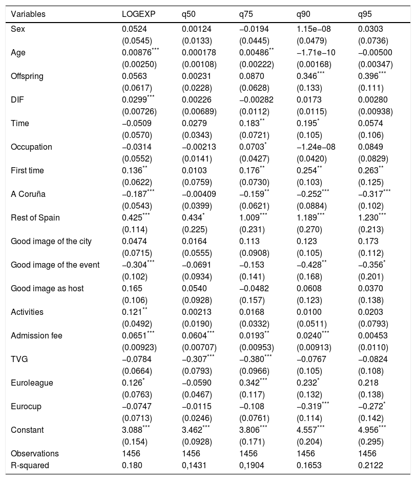
Table 2 shows the results of the model. The first column corresponds to the OLS regression and the following columns show the regressions of quantiles 50, 75, 90 and 95, respectively. The OLS regression contains 9 significant variables. The variables gender, good image of the city and good image of the host are not significant in the OLS, nor do they show any significance at the different quantiles.

Table 2.

Results of OLS and quantile regressions.

Variables	LOGEXP	q50	q75	q90	q95
Sex	0.0524	0.00124	−0.0194	1.15e−08	0.0303
	(0.0545)	(0.0133)	(0.0445)	(0.0479)	(0.0736)
Age	0.00876^***	0.000178	0.00486^**	−1.71e−10	−0.00500
	(0.00250)	(0.00108)	(0.00222)	(0.00168)	(0.00347)
Offspring	0.0563	0.00231	0.0870	0.346^***	0.396^***
	(0.0617)	(0.0228)	(0.0628)	(0.133)	(0.111)
DIF	0.0299^***	0.00226	−0.00282	0.0173	0.00280
	(0.00726)	(0.00689)	(0.0112)	(0.0115)	(0.00938)
Time	−0.0509	0.0279	0.183^**	0.195^*	0.0574
	(0.0570)	(0.0343)	(0.0721)	(0.105)	(0.106)
Occupation	−0.0314	−0.00213	0.0703^*	−1.24e−08	0.0849
	(0.0552)	(0.0141)	(0.0427)	(0.0420)	(0.0829)
First time	0.136^**	0.0103	0.176^**	0.254^**	0.263^**
	(0.0622)	(0.0759)	(0.0730)	(0.103)	(0.125)
A Coruña	−0.187^***	−0.00409	−0.159^**	−0.252^***	−0.317^***
	(0.0543)	(0.0399)	(0.0621)	(0.0884)	(0.102)
Rest of Spain	0.425^***	0.434^*	1.009^***	1.189^***	1.230^***
	(0.114)	(0.225)	(0.231)	(0.270)	(0.213)
Good image of the city	0.0474	0.0164	0.113	0.123	0.173
	(0.0715)	(0.0555)	(0.0908)	(0.105)	(0.112)
Good image of the event	−0.304^***	−0.0691	−0.153	−0.428^**	−0.356^*
	(0.102)	(0.0934)	(0.141)	(0.168)	(0.201)
Good image as host	0.165	0.0540	−0.0482	0.0608	0.0370
	(0.106)	(0.0928)	(0.157)	(0.123)	(0.138)
Activities	0.121^**	0.00213	0.0168	0.0100	0.0203
	(0.0492)	(0.0190)	(0.0332)	(0.0511)	(0.0793)
Admission fee	0.0651^***	0.0604^***	0.0193^**	0.0240^***	0.00453
	(0.00923)	(0.00707)	(0.00953)	(0.00913)	(0.0110)
TVG	−0.0784	−0.307^***	−0.380^***	−0.0767	−0.0824
	(0.0664)	(0.0793)	(0.0966)	(0.105)	(0.108)
Euroleague	0.126^*	−0.0590	0.342^***	0.232^*	0.218
	(0.0763)	(0.0467)	(0.117)	(0.132)	(0.138)
Eurocup	−0.0747	−0.0115	−0.108	−0.319^***	−0.272^*
	(0.0713)	(0.0246)	(0.0761)	(0.114)	(0.142)
Constant	3.088^***	3.462^***	3.806^***	4.557^***	4.956^***
	(0.154)	(0.0928)	(0.171)	(0.204)	(0.295)
Observations	1456	1456	1456	1456	1456
R-squared	0.180	0,1431	0,1904	0.1653	0.2122

Standard errors in parentheses.

*

p < 0.1.

**

p < 0.05.

***

p < 0.01.

Age is significant for OLS and relates positively to expenditure: the higher the age, the greater the level of individual expenditure. In the quantile regression, age is only significant for q75.

Attending with offspring is not significant for OLS, but is significant for q90 and q95. The relationship between this variable and spending is positive. Attendees who come with their offspring incur the greatest individual expenditures. This fact is confirmed for the quantiles representing a higher level of spending.

The variable representing the score difference in the matches won against the visiting team is significant for OLS with a positive sign. This means that the greater the difference between the local and visiting teams, the more the attendees spend on average. However, this variable is not significant for any of the quantiles.

The time of the match is not significant for OLS. However, it is significant for quantiles q75 and q90. The relationship is positive and it shows that attendees spend more when the match takes place in the afternoon. Occupation is significant only for q75. It presents a positive relationship with the spending what means that for this quantile those that have a job spend more.

The price of admission is a significant variable in OLS and in quantiles q50, q75 and q90. The admission price does not have a significant impact on spending in the city by the spectators at the highest spending level (quantile q95).

The TVG variable represents whether or not the matches were broadcast on regional TV and TVE represents the broadcasting of the matches on the national TV. TVG is not significant for OLS but it is significant for quantiles q50 and q75. Attendees spend less when the match is broadcast on TVG than when it is broadcast on TVE. The matches broadcast on TVE are often the most appealing because either one or both of the teams are at the top of the league table.

The Euroleague variable is significant for OLS, and for quantiles q75 and q90. Its relation to expenditure is positive. This indicates that attendees who spend less than €71 spend more when the rival team is also competing in the Euroleague. However, the Eurocup variable has a negative coefficient, meaning that it shows the opposite behavior and it is significant for q90 and q95.

The origin of the attendees is significant for OLS, both for attendees coming from A Coruña as well as for those coming from the rest of Spain. The reference variable for this is attendees traveling from the rest of Galicia. Attendees from the rest of Spain spend more than those from the rest of Galicia, and the attendees coming from A Coruña spend less than those coming from the rest of Galicia. Origin is significant for national attendees in all quantiles and it is significant for provincial attendees in quantiles q75, q90 and q95. Origin is the spending determinant has the most impact on the highest spending levels.

Attendees who are coming for the first time tend to spend more than those who are repeating the experience. In the case under consideration, this variable is significant using OLS and in quantiles q75 and q95. The highest level of spending generates increased individual spending when attendees are watching a match for the first time.

The good image of the event variable is significant using OLS and for quantiles q90 and q95. There is a negative relationship with event image, i.e., those who have a worse perception of the event spend more. The dummy variables good Image of the city and good image as host are not significant for OLS, nor for the different quantiles.

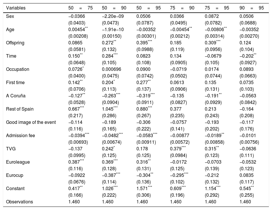
The result of the interquantile regression determines whether the difference between the different quantiles is significant (Table 3). To carry it out, only the variables that were significant in the quantile regression have been used. Demographic variables are included whether or not they are significant. The hypothesis posed is that of equality among quantiles. Significant indicators show that there are differences between the quantiles, analyzed in pairs. As may be seen in Table 3, the greatest number of significant determinants fall between quantiles q50 = q75, q50 = q90 and q50 = q95. It then follows that this is where the greatest number of hypotheses of equality among quantiles can be rejected. The number of significant variables decreases noticeably for the rest of the relationships between the quantiles. Thus, spending behavior between quantiles q75, q90 and q95 does not differ with respect to the different determinants analyzed.

Table 3.

Result of interquantile regression.

Variables	50 = 75	50 = 90	50 = 95	75 = 90	75 = 95	90 = 95
Sex	−0.0366	−2.20e−09	0.0506	0.0366	0.0872	0.0506
	(0.0403)	(0.0473)	(0.0787)	(0.0495)	(0.0782)	(0.0688)
Age	0.00454^**	−1.91e−10	−0.00352	−0.00454^**	−0.00806^**	−0.00352
	(0.00208)	(0.00150)	(0.00301)	(0.00212)	(0.00314)	(0.00270)
Offspring	0.0865	0.272^**	0.395^***	0.185	0.309^***	0.124
	(0.0581)	(0.132)	(0.0988)	(0.119)	(0.0956)	(0.104)
Time	0.150^**	0.284^***	0.0823	0.134	−0.0679	−0.202^**
	(0.0648)	(0.105)	(0.108)	(0.0905)	(0.105)	(0.0927)
Occupation	0.0726^*	0.000696	0.0900	−0.0719	0.0174	0.0893
	(0.0400)	(0.0475)	(0.0742)	(0.0502)	(0.0744)	(0.0663)
First time	0.142^**	0.204^*	0.277^**	0.0613	0.135	0.0735
	(0.0706)	(0.113)	(0.137)	(0.0906)	(0.131)	(0.103)
A Coruña	−0.127^**	−0.263^***	−0.319^***	−0.135	−0.191^**	−0.0563
	(0.0528)	(0.0904)	(0.0911)	(0.0827)	(0.0929)	(0.0842)
Rest of Spain	0.667^***	1.045^***	0.880^***	0.377	0.213	−0.164
	(0.217)	(0.286)	(0.267)	(0.235)	(0.243)	(0.208)
Good image of the event	−0.114	−0.189	−0.306	−0.0757	−0.193	−0.117
	(0.116)	(0.165)	(0.222)	(0.141)	(0.202)	(0.176)
Admission fee	−0.0394^***	−0.0482^***	−0.0583^***	−0.00877	−0.0189^**	−0.0101
	(0.00693)	(0.00674)	(0.00911)	(0.00572)	(0.00858)	(0.00756)
TVG	−0.137	0.242^*	0.178	0.379^***	0.315^**	−0.0636
	(0.0995)	(0.125)	(0.125)	(0.0984)	(0.123)	(0.111)
Euroleague	0.387^***	0.369^***	0.316^**	−0.0172	−0.0703	−0.0532
	(0.116)	(0.128)	(0.131)	(0.125)	(0.139)	(0.123)
Eurocup	−0.0922	−0.387^***	−0.304^**	−0.295^***	−0.212	0.0835
	(0.0676)	(0.114)	(0.136)	(0.102)	(0.132)	(0.117)
Constant	0.417^**	1.026^***	1.571^***	0.609^***	1.154^***	0.545^**
	(0.166)	(0.222)	(0.306)	(0.196)	(0.292)	(0.255)
Observations	1.460	1.460	1.460	1.460	1.460	1.460

Standard errors in parentheses.

*

p < 0.1.

**

p < 0.05.

***

p < 0.01.

From the results obtained from the quantile and interquantile regressions, two spending levels may be established. There is a clear difference between the influence of the determinants within q50 and the rest of the quantiles. The first level of spending consists of attendees who spend less than €32. The factors that influence this spending level are the admission price, match broadcasting and origin of attendees.

The second level of spending is established for quantiles q75, q90 and q95 (attendees who spend less than €152). The behavior of the various determinants is very similar for these three quantiles. Additionally, very few factors are observed to reject the hypothesis of equality throughout the interquantile regression. Spending is influenced by attendance with offspring, experience, origin and the image of the event. Concerning the sporting aspect, spending is higher when the match is in the evening, and it is influenced by the admission price as well as the league ranking of the rival team.

6

Discussion

By studying the determinants of spending, we can analyze the influence of attendee spending from a microeconomic point of view. This in turn enables the identification of patterns in spending behaviors, different spending segments, and the factors which generate these differences. In this sense, using spending determinants to study sporting events not only improves and deepens empirical analysis in sports event management, but it also represents a step forward in understanding sporting events from an economic perspective. This paper focuses on one type of sporting event that has not yet been discussed in the literature, and does so by identifying spending patterns. The main contribution of this paper is that it tests the response of spending behavior of attendees in league-type events using determinants directly related to sports aspects, which have rarely been considered before.

The analysis identifies the main determinants and their effects on individual spending for visitors attending Obradoiro matches. It formulates a model by applying linear and quantile regression. The latter has not been applied in previous works on spending determinants in sporting events. According to the results revealed by the quantile regressions, the determinants are found to change depending on how much the attendees spend.

Spending is not specially influenced by the sociodemographic variables in this case. The variable of gender does not have a significant relationship with spending in either the linear or quantile regressions. Thus, it would be pointless to establish specific programs to attract more women because gender represents no differences in spending level. Brida et al. (2011), Saayman and Saayman (2012) and Dixon et al. (2012) present similar results where the gender variable is not significant in relation to spending either. However, there is no unanimity with this regard, because in the studies by Sato et al. (2014) and Bilgic et al. (2008) gender is significant and men spend more than women.

Age is significant, and spending increases with age. Table 2 shows that variable AGE is significant for OLS and q75. Accordingly, could prove convenient focusing on specific age group of sports tourists when the target is to incentivize expenditure in the geographic area. This variable is probed to be significant only in the papers by Saayman and Saayman (2012) and Sato et al. (2014). In general, as stated by Saayman and Saayman (2012) the effect that socio-demographic variables produce depends on the type of sporting event.

The variable “offspring” is one of the variables that show the greatest impact on the quantile of higher expenditure levels. Therefore, the results suggest that individuals traveling with children spend more. This could suggest that there would be a potential niche market and that it would be important to develop family or child-directed activities to increase spending even more. Offspring is the variable that shows the greatest impact, following rest of Spain, for q95. Similar result appears in the paper of Brida et al. (2011) where it is stated that the presence of children under-12 generates a positive and significant effect on expenditure.

The origin of the visitors is an important variable in this analysis. It allows us to identify differences in how much is spent according to the area of origin (provincial, regional or national). The results show that these variables are significant. Rest of Spain is the variable that shows the greatest impact for q95. The spectators coming from the province of A Coruña (provincial) spent less than those coming from the rest of Galicia (regional) and the rest of Spain (national). Bilgic et al. (2008) also included the origin of attendees in their paper and they obtained a significant relationship identifying differences in the level of spending regarding the origin. Sato et al. (2014) using a variable to identify when the attendee comes from other countries also obtain a positive and significant influence in the spending.

Psychographic factors do not remarkably influence spending. Solely the good image of the event variable is significant for OLS and in quantiles q90 and q95, but their relationship to spending is inverted. This can be explained by the event dynamics. Attendants who only attend the match can have a good image of the event and not make more spending on tourism. In general, there is no unanimity regarding the influence of psychographic factors on expenditure, the previous studies obtain heterogeneous results.

Variables related to sporting aspects play an important role in terms of spending. The admission price is more meaningful to attendees who spend the least (quantile q50), while this influence decreases as spending increases and is not significant to spectators who spend more (quantile q95). Similarly, broadcasting affects spectators who spend less, but does not affect attendees who spend more in the city. This fact leads us to the conclusion that spectators who spend more usually have higher purchasing power and in consequence can afford to pay for more expensive tickets and do not care if the match is broadcast or not when deciding on whether to attend.

Scheduling also influences attendee spending. Spending is higher when the game takes place in the evening. The ranking of the sports team is also an aspect that plays a role in spending. Attendee spending is greater when the rival team plays in the Euroleague than if the home team is playing against a team that only plays in the Liga Endesa. Teams playing the Euroleague hold the highest league ranking. They thus attract a wider audience and the admission price to see them is higher.

The results obtained reveal that features associated with sport influence spending behavior. Matches against a team high up in the rankings or at a similar competitive level as the home team can attract non-habitual spectators. Those spectators are attracted by the spectacle and are not regular match attendees. This kind of attendee may follow different spending patterns compared to the regular spectator. Moreover, they may spend more. In this sense, from the results of this study, attendees going to a match for first time spend higher on average than those repeating the experience. Even though this is not enough to constitute evidence, it represents a first step to a more in-depth study of the differences in behavior between habitual spectators versus occasional ones.

As already noted, only a numbers of papers have included variables related to sport when studying determinants of spending in sport. Only Bilgic et al. (2008), Shani et al. (2010), Dixon et al. (2012) and Sato et al. (2014) do it. All of them confirm that the variables directly connected with the event have a significant effect on spending.

It can be concluded that in this study, the factor with the most significant influence on spending is the origin of the attendees. At the same time, it is shown that variables directly associated with the sporting aspects of the event influence the spending behavior of those attending Obradoiro team matches. Therefore, these characteristics should be considered when studying the determinants of sporting events. Future work could check how these variables respond in other sporting events, and consider sporting variables individually rather than as a part of other factors (motivational or touristic).

The results of the quantile and interquantile regressions identify two levels of spending. The identification of segments of expenditure and the factors influencing each one of them allows event organizers to decide on which segments and factors they should focus their actions. These measures could be related to the implementation of actions to attract spectators to matches or to incentivize spending in the stadium.

In the case of Obradoiro, tickets were not sold out. In that sense, still there is room for the development of strategies to attract spectators to the stadium. Thus, the organizers should focus their marketing efforts on attracting spectators in the highest expenditure segment. Two aspects become crucial. The first is the origin of the attendees. Marketing policy should focus on possible attendees from the rest of the provinces in Galicia and Spain. In this regard, this club has the advantage that no other teams in the region are playing in the top league. Thus, anybody living in Galicia who wants to attend live matches played by top-ranking basketball teams has to go to Santiago de Compostela.

Other measures could be taken in order to increase the expenditure of those coming to Santiago de Compostela. Especially for those coming from the rest of Spain, discounts on complementary activities that can be done before or after the match would be a good incentive. This implies cooperation between the event organizers and the body responsible for developing tourism in the city. This could represent the implementation of strategies involving sectors that could benefit from them in the mid and long term, such as hostelry and retail.

In general, a deeper knowledge of the economic impact of an event provides useful information for decision-making. Public authorities should be the first interested in this type of information and use it to improve tourism strategies jointly with other areas such as sports. Sports events allow the attraction of attendees that can take advantage of the trip to enjoy tourism activities. For that reason, it is important to facilitate the attendees with the opportunity of carrying out other activities complementary to the event. In this regard, public authorities can participate actively together with the tourism industry.

7

Conclusions

Our findings provide in-depth knowledge on the spending behavior of visitors attending Obradoiro matches. We have decided to work with total expenditure and not with daily expenditure to gather the influence on spending for those that need or decide to spend more time in the city. This information allows managers to plan event strategies focused on specific segments of attendees according to how much they spend. Moreover, it can contribute to the plan of cooperation with tourism institutions in the territory in order to incentivize attendees to spend more time in the city.

Studying the determinants of expenditure generally makes it easier to both estimate the economic impact of events and to identify useful information for the decision-making process when considering attendee spending behavior at sporting event destinations. These types of studies have implications for scientific research contributing to knowledge on sports tourism. On the other hand, they also have important practical implications in terms of developing marketing and financial strategies for sports events and promoting tourism for specific territories via sporting events.

This work has the advantage of the wide database considering the number of observations. However, it has the limitation that the survey was carried out only for one club during one season. So it would be interesting to analyze data from different clubs over several seasons. We consider this interesting for future research. It will help to deepen the study of the spending profiles of attendees at sporting events. Including factors directly related to the event could enable some prediction of spending patterns and then the subsequent economic impact.

Acknowledgements

The study was implemented in the framework of the Basic Research Program at the National Research University Higher School of Economics (HSE) in 2017.

We want to express our gratitude with Xosé Antón Antelo for his work with the survey and to Club Obradoiro for helping us to gather the information needed for this study.